R Recipes: A Problem-Solution Approach (2014)

Chapter 11. Relationships Between and Among Variables

In Chapter 11, you learn how to examine and test the significance of relationships between two or more variables measured at the scale (interval and ratio), ordinal, and nominal levels. The study of relationships is an important part of statistics, because we use correlational studies to answer important research questions in a variety of disciplines.

We begin with correlation and regression, examining relationships between a single predictor and a single criterion or dependent variable. We then move to special cases of the correlation coefficient that involve ranked or nominal data for one or both of the variables. Next, we expand the discussion to include a brief introduction to multiple correlation and regression, and we show the importance of this very general technique by relating it to the hypothesis tests we studied in Chapter 10.

Recipe 11-1. Determining Whether Two Scale Variables Are Correlated

Problem

Francis Galton developed the concept of correlation, but left his protégé Karl Pearson to work out the formula. We find that many variables are related to each other in a linear fashion, but correlation does not prove causation. For example, Galton measured various characteristics of more than 9,000 people, including their head circumference. His belief was that people with larger heads must have larger brains and that people with larger brains must be more intelligent. That hypothesis was refuted for years, but recent analyses have shown that indeed there is a small but significant relationship between brain volume and intelligence. A study of more than 1,500 people in 37 samples produced an estimate of the population correlation between the volume of the brain measured in vivo by MRI and an intelligence of .33. Correlation and regression are used in many disciplines to model linear relationships between two or more variables. We begin with the bivariate case for scale data and then study variations on the correlation coefficient for examining relationships when the variables are not measured on a scale.

The correlation coefficient can be understood best by first understanding the concept of covariation. The covariance of x (the predictor) and y (the criterion) is the average of the cross-products of their respective deviation scores for each pair of data points. The covariance, which we will designate as σ_xy, can be positive, zero, or negative. In other words, the two variables may be positively related (they both go up together and down together); not at all related; or negatively related (one variable goes up while the other goes down). The population covariance is defined as follows:

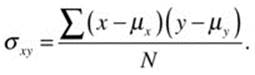
where N is the number of pairs of (x, y) data points. When we do not know the population mean, we substitute the sample mean and divide the sum of the cross-products of the deviation scores by n – 1 as a correction factor:

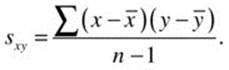
The covariance is a useful index, but it is affected by the units of measurement for x and y. The covariance of football players’ heights and weights expressed in centimeters and kilograms is different from the covariance expressed in inches and pounds. The correlation coefficient corrects this by dividing the covariance by the product of the standard deviations of x and y, resulting in an index that ranges from –1 through 0 to +1, representing a perfect negative relationship, no linear relationship, and a perfect positive relationship. The correlation between the players’ heights and weights is invariant whether the height units are inches or centimeters, and whether the weights are expressed in pounds or kilograms. In the population, we define the correlation coefficient as ρ (the Greek letter rho):

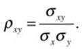
In the sample, we use the sample statistics as estimates of the population parameters.

Solution

Let us illustrate the “scalelessness” property of the correlation coefficient by working out the example used earlier. The following data represent the 2014 roster for the New Orleans Saints. Heights are recorded in inches and centimeters, and weights are recorded in pounds and kilograms.

> saints <- read.csv("saintsRoster.csv")
> head(saints)
Number Name Position Inches Pounds centimeters kilograms Age
1 72 Armstead, Terron T 77 304 195.58 138.18 23
2 61 Armstrong, Matt C 74 302 187.96 137.27 24
3 27 Bailey, Champ CB 73 192 185.42 87.27 36
4 36 Ball, Marcus S 73 209 185.42 95.00 27
5 9 Brees, Drew QB 72 209 182.88 95.00 35
6 34 Brooks, Derrius CB 70 192 177.80 87.27 26
Experience College
1 1 Arkansas-Pine Bluff
2 R Grand Valley State
3 16 Georgia
4 1 Memphis
5 14 Purdue
6 1 Western Kentucky
> tail(saints)
Number Name Position Inches Pounds centimeters kilograms Age
70 75 Walker, Tyrunn DE 75 294 190.50 133.64 24
71 42 Warren, Pierre S 74 200 187.96 90.91 22
72 82 Watson, Benjamin TE 75 255 190.50 115.91 33
73 71 Weaver, Jason T/G 77 305 195.58 138.64 25
74 60 Welch, Thomas T 79 310 200.66 140.91 27
75 24 White, Corey CB 73 205 185.42 93.18 24
Experience College
70 3 Tulsa
71 R Jacksonville State
72 11 Georgia
73 1 Southern Mississippi
74 4 Vanderbilt
75 3 Samford

Observe that the covariances between height and weight are different, depending on the units of measurement as we discussed before, but the correlations are the same (within rounding error) for height and weight, regardless of the measurement units. The covariance is found with thecov() function, and the correlation with the cor() function.

> cov(saints$Inches, saints$Pounds)
[1] 80.86685
> cov(saints$centimeters, saints$kilograms)
[1] 93.36248
> cor(saints$Inches, saints$Pounds)
[1] 0.6817679
> cor(saints$centimeters, saints$kilograms)
[1] 0.6817578

For the height and weight data, there is a positive correlation. The cor.test() function tests the significance of the correlation coefficient:

> cor.test(saints$Inches, saints$Pounds)

Pearson's product-moment correlation

data: saints$Inches and saints$Pounds
t = 7.9624, df = 73, p-value = 1.657e-11
alternative hypothesis: true correlation is not equal to 0
95 percent confidence interval:
0.5380635 0.7869594
sample estimates:
cor
0.6817679

With 73 degrees of freedom, the correlation is highly significant. The astute reader will notice that the significance of the correlation is tested with a t test.

The correlation coefficient can be used to calculate the intercept and the slope of the regression line, as follows. We will symbolize the intercept as b₀ and the regression coefficient (slope) as b₁. The slope is

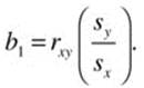
and the intercept is

See that the intercept will be the mean of y when the slope coefficient is zero. The lm() function (for linear model) will produce the coefficients. The t test in the bivariate case for the slope coefficient is equivalent to the t test for the overall regression, and the F ratio for the regression is the square of the t value.

> model <- lm(saints$Pounds ~ saints$Inches)
> summary(model)

Call:
lm(formula = saints$Pounds ~ saints$Inches)

Residuals:
Min 1Q Median 3Q Max
-68.877 -21.465 -1.282 19.351 104.579

Coefficients:
Estimate Std. Error t value Pr(>|t|)
(Intercept) -662.668 113.935 -5.816 1.48e-07 ***
saints$Inches 12.228 1.536 7.962 1.66e-11 ***
---
Signif. codes: 0 '***' 0.001 '**' 0.01 '*' 0.05 '.' 0.1 ' ' 1

Residual standard error: 33.97 on 73 degrees of freedom
Multiple R-squared: 0.4648, Adjusted R-squared: 0.4575
F-statistic: 63.4 on 1 and 73 DF, p-value: 1.657e-11

Recipe 11-2. Special Cases of the Correlation Coefficient

Problem

We often have data for x or y (or both) that are not interval or ratio, but we would still like to determine whether there is a relationship or association between the variables. There are alternatives to the Pearson correlation for such circumstances. We will examine the case in which one variable is measured on a scale while the other is measured as a dichotomy, where one or both variables are measured at the ordinal level, and where both variables are measured as dichotomies.

Solution

When you correlate a binary (0, 1) variable with a variable measured on a scale, you are using a special case of the correlation coefficient known as the point-biserial correlation. The computations are no different from those for the standard correlation coefficient. The binary variable might be the predictor x, or it might be the criterion y. When the binary variable is the predictor, the point-biserial correlation is equivalent to the independent-samples t test with regard to the information to be gleaned from the analysis. When the binary variable is the criterion, we are predicting a dichotomous outcome such as pass/fail. There are some issues with predicting a (0, 1) outcome using standard correlation and regression, and logistic regression offers a very attractive alternative that addresses these issues. When both variables are dichotomous, the index of relationship is known as the phi coefficient, and it has a relationship to chi-square, as you will learn.

Point-Biserial Correlation

Let us return to the example used for the independent-samples t test in Recipe 10-3. For this analysis, the data are reconfigured so that the dependent variable is the x scores followed by the y scores from the previous example. A 0 is used to indicate membership in x and a 1 is used to indicatey group membership.

> head(biserial)
newDV indicator
1 60.2 0
2 64.4 0
3 64.8 0
4 65.6 0
5 63.7 0
6 68.0 0
> tail(biserial)
newDV indicator
45 79.8 1
46 82.5 1
47 80.7 1
48 86.4 1
49 81.2 1
50 94.1 1

We can now regress the new dependent variable onto the column of zeros and ones by using the lm() function. The results will be instructive in terms of the relationship between the t test and correlation.

> biserialCorr <- lm(newDV ~ indicator, data = biserial)
> summary(biserialCorr)

Call:
lm(formula = newDV ~ indicator, data = biserial)

Residuals:
Min 1Q Median 3Q Max
-16.616 -4.691 -0.120 5.059 19.876

Coefficients:
Estimate Std. Error t value Pr(>|t|)
(Intercept) 65.824 1.647 39.958 < 2e-16 ***
indicator 18.692 2.330 8.024 2.03e-10 ***
---
Signif. codes: 0 '***' 0.001 '**' 0.01 '*' 0.05 '.' 0.1 ' ' 1

Residual standard error: 8.237 on 48 degrees of freedom
Multiple R-squared: 0.5729, Adjusted R-squared: 0.564
F-statistic: 64.38 on 1 and 48 DF, p-value: 2.029e-10

Now, compare the results from the linear model with the results of the standard t test assuming equal variances for x and y. Observe that the value of t testing the significance of the slope coefficient in the regression model is equivalent to the value of t comparing the means (ignoring the sign). The intercept term in the regression model is equal to the mean of x, and the slope coefficient is equal to the difference between the means of x and y. These equivalences are because both the correlation and the t test are based on the same underlying general linear model.

> t.test(x, y, var.equal = T)

Two Sample t-test

data: x and y
t = -8.0235, df = 48, p-value = 2.029e-10
alternative hypothesis: true difference in means is not equal to 0
95 percent confidence interval:
-23.37607 -14.00793
sample estimates:
mean of x mean of y
65.824 84.516

As you just saw, the use of a dichotomous predictor is equivalent to an independent-samples t test. However, when the criterion is dichotomous and the predictor is interval or ratio, problems often arise. The problem is that the regression equation can lead to predictions for the criterion that are less than 0 and greater than 1. These can simply be converted to 0s and 1s as an expedient, but a more elegant alternative is to use binary logistic regression rather than point-biserial correlation for this purpose. Let us explore these issues with the following data. The job satisfaction data we worked with in Chapter 10 have been modified to include two binary variables, which indicate whether the individual is satisfied overall (1 = yes, 0 = no) and whether the person was promoted (1 = yes, 0 = no).

> head(jobSat)
subject satisf perf alternatives investment satYes promoYes
1 1 52 61 low low 0 0
2 2 42 72 low low 0 1
3 3 63 74 low low 0 1
4 4 48 69 low low 0 0
5 5 51 65 low low 0 0
6 6 55 71 low low 0 0
> tail(jobSat)
subject satisf perf alternatives investment satYes promoYes
55 55 87 67 high high 1 0
56 56 80 75 high high 1 1
57 57 88 70 high high 1 0
58 58 79 71 high high 1 0
59 59 83 67 high high 1 0
60 60 80 73 high high 1 1

Say we are interested in determining the correlation between promotion and satisfaction. We want to know if those who are more satisfied are more likely to be promoted. Our criterion now is a dichotomous variable. We can regress this variable onto the vector of satisfaction scores using the lm() function. We see there is a significant linear relationship. Those who are more satisfied are also more likely to be promoted. The R² value indicates the percentage of variance overlap between satisfaction and promotion, which is approximately 14.8%. The product-moment correlation is the square root of the R² value, which is .385 because the slope is positive.

> predictPromo <- lm(promoYes ~ satisf, data = jobSat)
> summary(predictPromo)

Call:
lm(formula = promoYes ~ satisf, data = jobSat)

Residuals:
Min 1Q Median 3Q Max
-0.6705 -0.4584 -0.1031 0.4240 0.8816

Coefficients:
Estimate Std. Error t value Pr(>|t|)
(Intercept) -0.270122 0.229652 -1.176 0.24431
satisf 0.010225 0.003222 3.174 0.00241 **
---
Signif. codes: 0 '***' 0.001 '**' 0.01 '*' 0.05 '.' 0.1 ' ' 1

Residual standard error: 0.4652 on 58 degrees of freedom
Multiple R-squared: 0.148, Adjusted R-squared: 0.1333
F-statistic: 10.07 on 1 and 58 DF, p-value: 0.002409

Using the coefficients from our linear model, we can develop a prediction for each employee’s promotion from his or her satisfaction score. The predict(lm) function performs this operation automatically.

> predict <- predict(lm(promoYes ~ satisf, data = jobSat))
> predict <- round(predict,2)
> jobSat <- cbind(jobSat, predict)
> head(jobSat)
subject satisf perf alternatives investment satYes promoYes predict
1 1 52 61 low low 0 0 0.26
2 2 42 72 low low 0 1 0.16
3 3 63 74 low low 0 1 0.37
4 4 48 69 low low 0 0 0.22
5 5 51 65 low low 0 0 0.25
6 6 55 71 low low 0 0 0.29

> summary(jobSat$predict)
Min. 1st Qu. Median Mean 3rd Qu. Max.
0.0200 0.2575 0.5100 0.4347 0.5800 0.6900

In the current case, the predicted values for promotion are all probabilities between 0 and 1. Note, however, that this is not always the case. In many situations, when you are predicting a binary outcome, the predicted values will be lower than 0 or greater than 1, as mentioned earlier. A preferable alternative in such cases is binary logistic regression. Use the glm() function (for general linear model) to perform the binary logistic regression. We create a model called myLogit and then obtain the summary.

> myLogit <- glm(promoYes ~ satisf, data = jobSat, family = "binomial")
> summary(myLogit)

Call:
glm(formula = promoYes ~ satisf, family = "binomial", data = jobSat)

Deviance Residuals:
Min 1Q Median 3Q Max
-1.5272 -1.0785 -0.5136 1.0394 2.0143

Coefficients:
Estimate Std. Error z value Pr(>|z|)
(Intercept) -3.77399 1.33523 -2.826 0.00471 **
satisf 0.04964 0.01791 2.771 0.00559 **
---
Signif. codes: 0 '***' 0.001 '**' 0.01 '*' 0.05 '.' 0.1 ' ' 1

(Dispersion parameter for binomial family taken to be 1)

Null deviance: 82.108 on 59 degrees of freedom
Residual deviance: 72.391 on 58 degrees of freedom
AIC: 76.391

Number of Fisher Scoring iterations: 3

This model is also significant. We see that for approximately every unit increase in job satisfaction, the log odds of promotion versus nonpromotion increase by .05.

The Phi Coefficient

The phi coefficient is a version of the correlation coefficient in which both variables are dichotomous. We also use the phi coefficient as an effect-size index for chi-square for 2 × 2 contingency tables. In this case, correlating the columns of zeros and ones is an equivalent analysis to conducting a chi-square test on the 2 × 2 contingency table. The relationship between phi and chi-square is as follows, where N is the total number of observations. First, we calculate the standard correlation coefficient with the two dichotomous variables, and then we calculate chi-square and show the relationship.

> cor.test(jobSat$satYes, jobSat$promoYes)

Pearson's product-moment correlation

data: jobSat$satYes and jobSat$promoYes
t = 3.4586, df = 58, p-value = 0.001024
alternative hypothesis: true correlation is not equal to 0
95 percent confidence interval:
0.1782873 0.6039997
sample estimates:
cor
0.4134925

The value of chi-square (without the Yates continuity correction) is as follows:

> chisq.test(table(jobSat$satYes, jobSat$promoYes), correct = F)

Pearson's Chi-squared test

data: table(jobSat$satYes, jobSat$promoYes)
X-squared = 10.2586, df = 1, p-value = 0.001361

Apart from rounding error, the phi coefficient is equal to the correlation that we calculated previously.

> phi <- sqrt(10.2586/60)
> phi
[1] 0.4134932

The Spearman Rank Correlation

The Spearman Rank Correlation, r_s, (also known as Spearman’s Rho) is the nonparametric version of the correlation coefficient for variables measured at the ordinal level. Technically, this index measures the degree of monotonic increasing or decreasing relationship instead of linear relationship. This is because ordinal measures do not provide information concerning the distances between ranks. Some data are naturally ordinal in nature, while other data are converted to ranks because the data are nonnormal in their distribution.

As with the phi coefficient, r_s can be calculated using the formula for the product moment coefficient after converting both variables to ranks. The value of r_s is calculated as follows:

where d_i = x_i – y₁ is the difference between ranks for a given pair of observations. The cor.test() function in R provides the option for calculating Spearman’s r_s. To illustrate, let us examine the relationship between the job satisfaction and job performance. See that when we choose the argument method = "spearman" for the cor.test() function, the result is identical to the standard correlation between the ranks for the two variables.

> cor.test(jobSat$satisf, jobSat$perf, method = "spearman")

Spearman's rank correlation rho

data: jobSat$satisf and jobSat$perf
S = 20906.99, p-value = 0.0008597
alternative hypothesis: true rho is not equal to 0
sample estimates:
rho
0.4190888

Warning message:
In cor.test.default(jobSat$satisf, jobSat$perf, method = "spearman") :
Cannot compute exact p-value with ties

Now, examine the result of correlating the two sets of ranks:

> cor.test(rank(jobSat$satisf), rank(jobSat$perf))

Pearson's product-moment correlation

data: rank(jobSat$satisf) and rank(jobSat$perf)
t = 3.5153, df = 58, p-value = 0.0008597
alternative hypothesis: true correlation is not equal to 0
95 percent confidence interval:
0.1848335 0.6082819
sample estimates:
cor
0.4190888

Recipe 11-3. A Brief Introduction to Multiple Regression

Problem

In many research studies, there is a single dependent (criterion) variable but multiple predictors. Multiple correlation and regression apply in cases of one dependent variable and two or more independent (predictor or explanatory) variables. Multiple regression takes into account not only the relationships of each predictor to the criterion, but the intercorrelations of the predictors as well. The multiple linear regression model is as follows:

This means that the predicted value of y is a linear combination of an intercept term added to a weighted combination of the k predictors. The regression coefficients, symbolized by b, are calculated in such a way that the sum of the squared residuals (the differences between the observed and predicted values of y) is minimized. The multiple correlation coefficient, R, is the product-moment correlation coefficient between the observed and predicted y values. Just as in bivariate correlation and regression, R² shows the percentage of variation in the dependent (criterion) variable that can be explained by knowing the value of the predictors for each individual or object.

Finding the values of the regression coefficients and testing the significance of the overall regression allows us to determine the relative importance of each predictor to the overall regression, and whether a given variable contributes significantly to the prediction of y. We use multiple regression in many different applications.

Solution

Multiple regression is a very general technique. ANOVA can be seen as a special case of multiple regression, just as the independent-samples t test can be seen as a special case of bivariate regression. Let us consider a common situation. We would like to predict college students’ freshman grade point average (GPA) from a combination of motivational and academic variables.

The following data are from a large-scale retention study I performed for a private liberal arts university. Data were gathered from incoming freshmen over a three-year period from 2005 to 2007. Academic variables included the students’ high school GPAs, their freshman GPAs, their standardized test scores (ACT and SAT), and the students’ rank in their high schools’ graduating class, normalized by the size of the high school. Motivational variables included whether the student listed this university first among the schools to receive his or her standardized test scores (preference) and how many hours the student attempted in his or her first semester as a freshman. Another motivational variable was whether the student was the recipient of an athletic scholarship. Demographic variables included the students’ sex and ethnicity. The data are as follows:

> head(gpa)
id pref frYr frHrs female hsGPA collGPA retained ethnic SATV SATM SAT ACT
1 17869 1 2006 15.5 1 4.04 2.45 1 1 480 530 1010 18
2 17417 1 2005 19.0 1 4.20 2.89 0 0 520 570 1090 20
3 16681 1 2006 15.0 1 4.15 2.60 1 1 400 410 810 18
4 17416 1 2005 16.5 1 4.50 3.39 1 1 490 480 970 23
5 16990 1 2005 17.0 1 3.83 2.65 1 1 440 460 900 18
6 16254 1 2006 15.0 1 4.32 1.93 1 1 450 650 1100 22
hsRank hsSize classPos athlete
1 129 522 0.75 0
2 35 287 0.88 0
3 9 13 0.31 0
4 6 158 0.96 0
5 94 279 0.66 0
6 23 239 0.90 0
> tail(gpa)
id pref frYr frHrs female hsGPA collGPA retained ethnic SATV SATM SAT
290 17019 1 2006 17 1 3.76 1.57 1 1 480 590 1070
291 18668 1 2007 15 1 4.24 2.80 1 1 540 480 1020
292 18662 1 2007 15 0 3.31 2.33 1 1 440 570 1010
293 19217 1 2007 16 0 4.54 2.25 1 1 540 470 1010
294 16041 1 2005 16 0 3.55 2.69 1 1 540 570 1110
295 18343 1 2007 16 1 4.21 3.31 1 1 530 660 1190
ACT hsRank hsSize classPos athlete
290 18 133 297 0.55 0
291 24 34 243 0.86 0
292 17 179 306 0.42 1
293 20 7 12 0.42 0
294 22 218 498 0.56 1
295 27 32 301 0.89 0

The lm() function in base R can be used for multiple regression. Let us create a linear model with the college GPA as the criterion and the academic variables of SAT verbal, SAT math, high school GPA, and class position as predictors. We can also add sex, preference, and status as a student athlete as predictors. We will run the full model and then eliminate any predictors that do not add significantly to the overall regression.

> mulReg <- lm(collGPA ~ SATV + SATM + hsGPA + classPos + female + pref + athlete, data = gpa)
> summary(mulReg)

Call:
lm(formula = collGPA ~ SATV + SATM + hsGPA + classPos + female +
pref + athlete, data = gpa)

Residuals:
Min 1Q Median 3Q Max
-1.2170 -0.3267 0.0130 0.3253 1.4529

Coefficients:
Estimate Std. Error t value Pr(>|t|)
(Intercept) 0.2207168 0.2874792 0.768 0.44326
SATV 0.0015583 0.0005095 3.059 0.00243 **
SATM 0.0003460 0.0005027 0.688 0.49178
hsGPA 0.2620812 0.0986011 2.658 0.00830 **
classPos 1.0528486 0.2416664 4.357 1.84e-05 ***
female 0.1714455 0.0704189 2.435 0.01552 *
pref -0.2986353 0.1164998 -2.563 0.01088 *
athlete 0.0574808 0.0772814 0.744 0.45761
---
Signif. codes: 0 '***' 0.001 '**' 0.01 '*' 0.05 '.' 0.1 ' ' 1

Residual standard error: 0.5136 on 287 degrees of freedom
Multiple R-squared: 0.4433, Adjusted R-squared: 0.4297
F-statistic: 32.64 on 7 and 287 DF, p-value: < 2.2e-16

The significant predictors are SAT verbal, high school GPA, class position, sex, and stated preference for this university. Let us run the regression again using only those predictors. Normally, we eliminate the nonsignificant variables one at a time; that is, we exclude the predictor with the highest p-value first, but here we eliminate both SATM and the athlete variable at the same time for illustrative purposes, as the p-values are quite similar.

> mulReg2 <- lm(collGPA ~ SATV + hsGPA + classPos + female + pref, data = gpa)
> summary(mulReg2)

Call:
lm(formula = collGPA ~ SATV + hsGPA + classPos + female + pref,
data = gpa)

Residuals:
Min 1Q Median 3Q Max
-1.2199 -0.3445 0.0213 0.3131 1.4816

Coefficients:
Estimate Std. Error t value Pr(>|t|)
(Intercept) 0.3182779 0.2730307 1.166 0.244688
SATV 0.0016898 0.0004428 3.816 0.000166 ***
hsGPA 0.2663688 0.0960505 2.773 0.005912 **
classPos 1.0850437 0.2395356 4.530 8.65e-06 ***
female 0.1517149 0.0680608 2.229 0.026575 *
pref -0.3008454 0.1152196 -2.611 0.009497 **
---
Signif. codes: 0 '***' 0.001 '**' 0.01 '*' 0.05 '.' 0.1 ' ' 1

Residual standard error: 0.5129 on 289 degrees of freedom
Multiple R-squared: 0.4408, Adjusted R-squared: 0.4312
F-statistic: 45.57 on 5 and 289 DF, p-value: < 2.2e-16

The value of R² is basically unchanged, and our new model uses only predictors that each contribute significantly to the overall regression. The predictors are highly interrelated, as the following correlations show, so we are interested in finding a combination of predictors that are each related to the criterion independently.

We can apply the regression equation we created to get predicted values of the college GPA, along with a 95% confidence interval using the predict.lm function. Remember the product-moment correlation between the predicted y values and the observed y values is multiple R, as the following output shows. The predict.lm function will optionally provide a confidence interval for each fitted value of y, giving the lower and upper bounds for the mean y for a given x. You can also specify a prediction interval, which will give the prediction limits for the range of individual y scores for a given x score. See that the predict.lm() function produces a matrix. Squaring the correlation between the fitted values and the observed y values produces the value of R² reported earlier.

> gpa.fit <- predict.lm(mulReg2, interval = "confidence")
> head(gpa.fit)
fit lwr upr
1 2.870169 2.788140 2.952199
2 3.121436 3.038125 3.204747
3 2.286866 2.010149 2.563582
4 3.237456 3.128370 3.346542
5 2.648985 2.553701 2.744270
6 3.056815 2.945514 3.168115
> cor(gpa.fit[,1], gpa$collGPA)^2
[1] 0.4408457

Our linear model is as follows.

This formula produces the fitted value of 2.8702 as the predicted value of the college GPA for the first student in the dataset. The interpretation of the confidence interval is that we are 95% confident that students with the same SAT verbal score, the same high school GPA, the same class position, and the same stated preference as this student will have college GPAs between 2.788 and 2.952.