R Recipes: A Problem-Solution Approach (2014)
Chapter 12. Contemporary Statistical Methods
You learned the traditional tests for differences in Chapter 10 and for relationships in Chapter 11. In Chapter 12, you will learn some of the modern statistical methods developed over the past half century. You have learned by now that statistics is not a static field, but a growing, dynamic, and evolving one. With modern technology, statisticians are able to perform calculations and analyses not previously available. The notion of sampling from a population and estimating parameters is still an important one, but newer techniques that allow us to use samples in new ways are increasingly available.
In Chapter 12, you will learn about modern robust statistical techniques that allow us to resample our data repeatedly and build the distribution of a statistic of interest, perhaps even one of our own creation. We can also simulate data and make inferences concerning various statistics. We can use techniques that improve our ability to make correct inferences when data distributions depart from normality. It is also possible to use permutation tests as alternatives to traditional hypothesis tests.
The disenchantment with null hypothesis significance testing began soon after R. A. Fisher suggested the technique in the first place. Fisher asserted that one does not (ever) need an alternative hypothesis. Instead, one examines a sample of data under the assumption of some population distribution, and determines the probability that the sample came from such a population. If the probability is low, then one rejects the null hypothesis. If the probability is high, the null hypothesis is not rejected. The notion of an alpha or significance level was important to Fisher’s formulation, but the idea of a Type II error was not considered. Fisher also developed the notion of a p value as an informal, but useful, way of determining just how likely it was that the sample results occurred by chance alone.
Karl Pearson’s son Egon Pearson and Jerzy Neyman developed a different form of hypothesis testing. In their framework, two probabilities were calculated, each associated with a competing hypothesis. The hypothesis that was chosen had the higher probability of having produced the sample results. Thus, the Neyman-Pearson formulation considered (and calculated) both Type I and Type II errors. Fisher objected to the Neyman-Pearson approach, and a bitter rivalry ensued. The rivalry ended with Fisher’s death in 1962, but the controversy endures.
Current hypothesis testing is an uneasy admixture of the Fisher and Neyman-Pearson approaches. The debate between these two approaches has been pursued on both philosophical and mathematical grounds. Mathematicians claim to have resolved the debate, while philosophers continue to examine the two approaches independently. However, an alternative is emerging that may soon supplant both of these approaches. These newer methods provide one the ability to make better, that is, more accurate and more powerful, inferences when data do not meet parametric distributional assumptions such as normality and equality of variance.
Recipe 12-1. Resampling Techniques
Problem
Many statistical problems are intractable from the perspective of traditional hypothesis testing. For example, making inferences about the distribution of certain statistics is difficult or impossible using traditional methods. Examine the histogram in Figure 12-1, which represents the hypothetical scores of 20 elderly people on a memory test. The data are clearly not normal. As the histogram indicates, some of the subjects have lost cognitive functioning. The problem is how to develop a confidence interval for the median of the data. It is clear how to develop a confidence interval for a mean, but what about a confidence interval for the median? Here are the 20 memory scores.
Memory <- c(2.5, 3.5, 4.5, 5.5, 6.5, 6.5, 6.5, 8.5, 8.5, 9.5, 9.5, 9.5, 9.5, 10.5, 10.5, 10.5, + 10.5, 11.5, 11.5, 12.5)
> breaks <- seq(2, 14, 1)
> hist(memory, breaks)
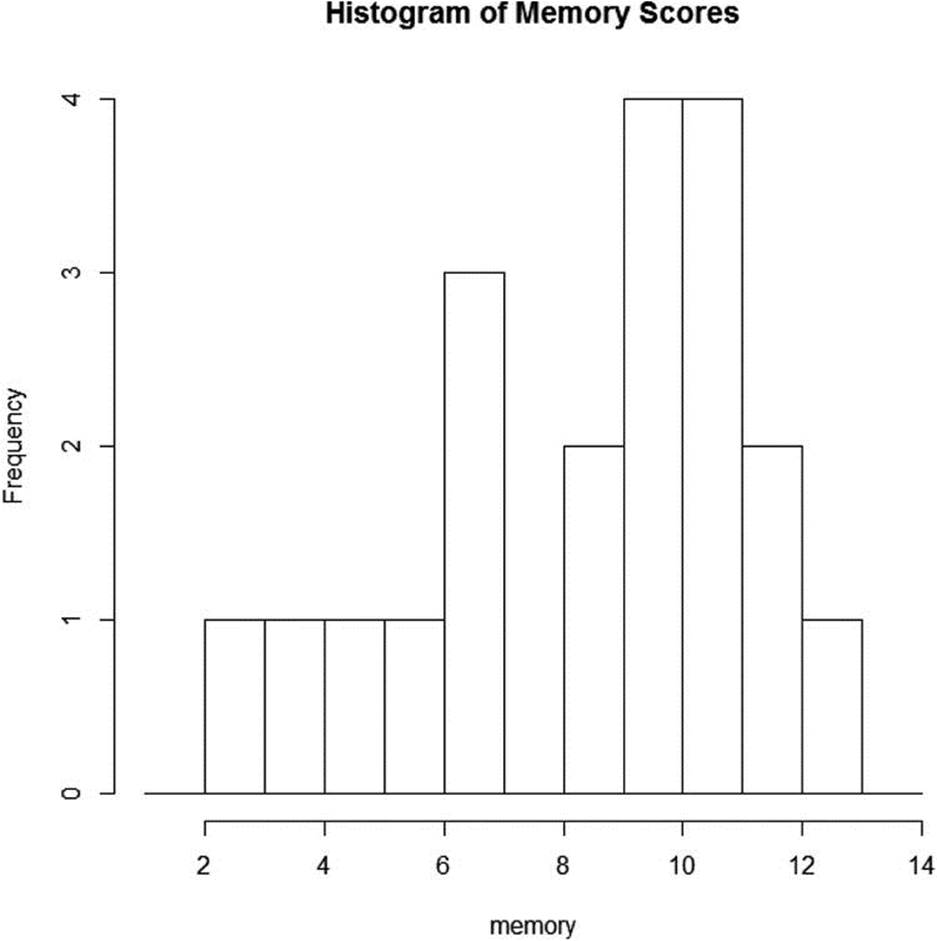
Figure 12-1. Hypothetical memory data for 20 elderly people
Solution
The solution in not as difficult as one might imagine. We treat the sample of 20 as a “pseudo-population,” and take repeated resamples with replacement from our original sample. We then calculate the median of each sample and study the distribution of sample medians. We can find the 95% confidence limits from that distribution using R’s quantile() function. Let us generate 10,000 resamples and calculate the median of each. Then we will generate a histogram of the distribution of the medians, followed by the calculation of the limits of the 95% confidence interval for the median. There are many ways to do this, but we can simply write a few lines of R code that loop explicitly through 10,000 iterations, taking a sample with replacement each time, and calculating and storing the median of each sample. Here is our R code. The numeric() command makes an empty vector that we then fill with the medians from each of the 10,000 resamples. The sampling with replacement is accomplished by setting the replace argument to T or TRUE.
nSamples <- 10000
medianSamp <- numeric()
for (i in 1:nSamples) medianSamp[i] <- median(sample(memory, replace = T))
hist(medianSamp)
(llMedian <- quantile(medianSamp, 0.025))
(ulMedian <- quantile(medianSamp, 0.975))
The histogram of the medians appears in Figure 12-2. Just as the original sample was negatively skewed, so is our distribution of medians.
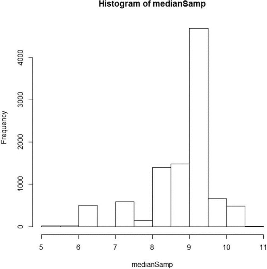
Figure 12-2. Histogram of 10,000 medians from resampling the “pseudo-population”
The 95% confidence interval for the median is [6.5, 10.5].
> (llMedian <- quantile(medianSamp, 0.025))
2.5%
6.5
> (ulMedian <- quantile(medianSamp, 0.975))
97.5%
10.5
The essence of all resampling techniques is the same as what we have done here. We use a sample of data and take a large number of resamples with replacement. We then study the distribution of the statistic of interest. This general approach is known as bootstrapping. The bootstrapping method can be used for other statistics simply by altering the R code. For example, we can study the distribution of the sample variance, the mean, or any other statistic we want without assuming anything about the population.
Recipe 12-2. Making Inferences About Means from Real Data
Problem
Real data are very unlikely to be normally distributed. Indeed, the parametric assumptions for t tests and ANOVA are often not met. When we make inferences about means and are unwilling to assume the population is normal, or that the variances in the population are equal, modern robust statistical methods can be very helpful. This approach was championed and described by Rand Wilcox in his articles and books on contemporary statistical methods. Wilcox has developed the WRS (Wilcox’ Robust Statistics) package, with more than 1,100 functions for various robust statistical calculations. The WRS package is not available through CRAN because of the lack of complete documentation for all functions, but it can be obtained from GitHub or through Wilcox’s web site at http://dornsife.usc.edu/labs/rwilcox/software/.
You will need to download this package if you wish to try out some of the functions that are used in the examples that follow. In general, a statistic is said to be robust to the extent that it performs well when the data are not normally distributed or when two or more samples have widely differing variances. Another concern with real data is that statistics such as the mean are heavily influenced by the presence of outliers. The median, on the other hand, is a robust statistic for estimating the central tendency of a data distribution because it is unaffected by extreme values. To elaborate further on the idea of robustness, Mosteller and Tukey defined two types, resistance and efficiency. A statistic (for example, the median) is resistant if changing a small part of the data (even by a large amount) does not lead to a large change in the estimate. A statistic has robustness of efficiency, on the other hand, if the statistic has high efficiency in a variety of situations, rather than a single situation. For example, the mean and variance, which are used as the basis for standard confidence intervals, do not have robustness of efficiency because they work well in this capacity only when data are normally distributed or when sample sizes are large.
Solution
The standard t test discussed in Chapter 10 is useful for comparing means when the data are sampled from normal distributions and when the variances are equal in the population. The Welch t test (the R default) is a better alternative when the population variances cannot be assumed to be equal. However, both versions of the t test are ineffective when the data differ substantially from a normal distribution—that is, when the distributions are highly skewed, as is often the case with real data (especially if the data have not been cleaned).
Trimmed means remove outliers by excluding a certain percentage of values at the high and low ends of the data distribution, and then calculating the mean of the remaining data values. Similarly, we can calculate Winsorized statistics. Winsorizing (named after Charles P. Winsor, who suggested the technique) is slightly more complicated than trimming. Winsorizing is defined as follows: the k-th Winsorized mean is the average of the observations after each of the first k smallest values are replaced by the (k + 1)th smallest value, and the k largest values are replaced by the (k + 1)th largest value. Thus, Winsorizing does not discard data values, as trimming does, but replaces data values with other observed values that are closer to the center of the data distribution.
The mean and the variance are used as the basis of confidence intervals, and by our definitions, they are efficient when the data are from a normal population. However, these statistics do not possess robustness of efficiency or resistance. Therefore, we would like to find estimators of the population mean that are both resistant and possess robustness of efficiency. We can develop confidence limits for a trimmed mean or for the differences between trimmed means. These techniques are robust alternatives to the standard one-sample and two-sample t tests.
Calculating and examining trimmed means is one alternative to the standard or Welch t test. A common approach is to use a 10% trimmed mean, therefore excluding the upper 10% and the lower 10% of observations. The mean function in R can be used to calculate the trimmed mean of a set of numbers. For example, let us calculate the trimmed mean for the numbers we used in Recipe 12-1. With 20% trimming, the trimmed mean is closer to the median than the original mean was, though even with trimming, the trimmed data are still negatively skewed, as the trimmed mean is lower than the median. The median is resistant, but has less robustness of efficiency than a trimmed or Winsorized mean because these statistics use more information than does the median.
We can calculate the variance for a trimmed mean as follows:
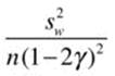
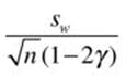
where σw2 is the Winsorized variance as discussed earlier, n is the sample size before trimming, and γ is the proportion of trimming. We can then calculate the standard error of the trimmed mean as
Wilcox’s WRS package includes a tmean function for calculating the trimmed mean, a trmse function for estimating the standard error of the trimmed mean, a win function for calculating a Winsorized mean, and a winvar function for calculating a Winsorized variance. The following code shows these functions applied to the memory data from Recipe 12-1. Observe that the built-in mean function produces the same answer as Wilcox’s tmean function, where the trimming proportion is the same. Note also that the trimming substantially reduced the variance of the trimmed data.
> mean(memory)
[1] 8.4
> mean(memory, trim = .2)
[1] 8.833333
> tmean(memory, tr = .2)
[1] 8.833333
> trimse(memory, tr = .2)
[1] 0.6578363
> win(memory, tr = .2)
[1] 8.7
> winvar(memory, tr = .2)
[1] 3.115789
> var(memory)
[1] 7.989474
We can also get a confidence interval for the trimmed mean by using Wilcox’s function trimci. This can substitute for a one-sample t test when the data are not normally distributed. If the test value (the hypothesized population mean) is within the limits of the confidence interval, we conclude that the evidence suggests that the sample came from a population with μ0.
> trimci(memory, tr = .2, alpha = .05)
[1] "The p-value returned by the this function is based on the"
[1] "null value specified by the argument null.value, which defaults to 0"
$ci
[1] 7.385445 10.281221
$estimate
[1] 8.833333
$test.stat
[1] 13.42786
$se
[1] 0.6578363
$p.value
[1] 3.63381e-08
$n
[1] 20
Now, assume that we locate a sample of elderly people who take a memory-enhancing supplement. We want to compare the means of the two groups (labeled memory1 and memory2). We note that the memory scores for the first group are negatively skewed and that the scores for the second group are positively skewed (see Figure 12-3). We find further that the variances of the two groups are not equal.
> memory1
[1] 2.5 3.5 4.5 5.5 6.5 6.5 6.5 8.5 8.5 9.5 9.5 9.5 9.5 10.5 10.5
[16] 10.5 10.5 11.5 11.5 12.5
> memory2
[1] 5.5 5.5 6.0 6.0 6.0 7.5 7.5 7.5 7.5 7.5 7.5 10.0 10.0 11.0 13.0
[16] 14.0 16.0 16.0 16.0 20.0
>
[1] 8.4
> mean(memory2)
[1] 10
> var(memory1)
[1] 7.989474
> var(memory2)
[1] 18.94737
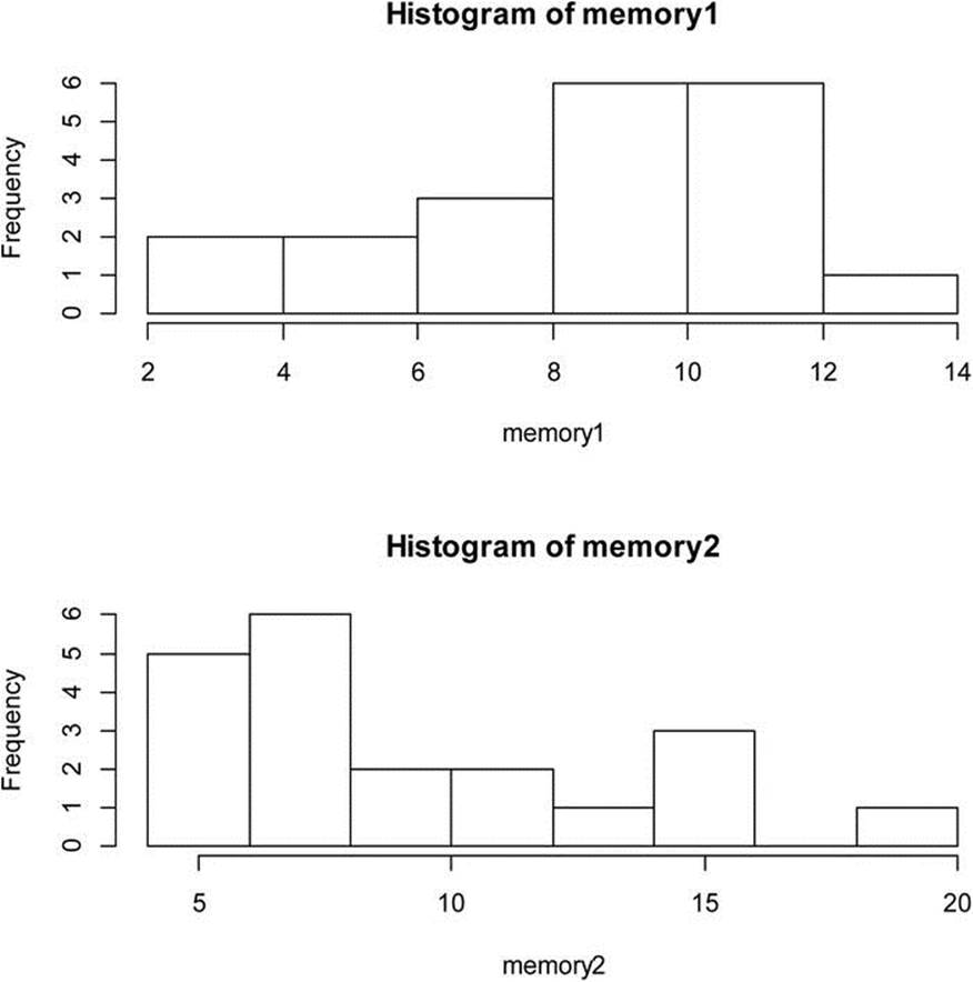
Figure 12-3. Comparison of memory scores of two groups of elderly persons
A robust alternative to the two-sample t test was developed by Yuen. The Yuen t statistic is the difference between the two trimmed means divided by the estimated standard error of the difference between the trimmed means,
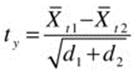
where the standard error estimates,
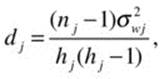
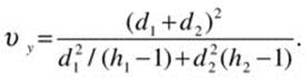
and the variance estimate, σwj2, is the γ-Winsorized variance for group j, and hj is the effective sample size after trimming. The degrees of freedom for the Yuen test are calculated as
Wilcox’s function yuen performs this test. Let us compare the results of the Welch test and the Yuen test to determine the effect of trimming on the resulting confidence intervals.
> t.test(memory1, memory2)
Welch Two Sample t-test
data: memory1 and memory2
t = -1.3787, df = 32.604, p-value = 0.1774
alternative hypothesis: true difference in means is not equal to 0
95 percent confidence interval:
-3.9622155 0.7622155
sample estimates:
mean of x mean of y
8.4 10.0
The yuen function produces a list as its output, so we will create an object and query the results for the confidence interval and p-value. The yuen function defaults to a trimming value of 0.20 and an alpha level of 0.05.
> yuenTest <- yuen(memory1, memory2)
> yuenTest$ci
[1] -3.215389 2.715389
> yuenTest$p.value
[1] 0.8609031
When the sample size is small, as it is in this case, a preferable alternative is to use a bootstrapped version of Yuen’s robust t test. Wilcox provides a function yuenbt to calculate a percentile-t bootstrap that estimates a confidence interval for the difference between two trimmed means. As with any hypothesis testing situation where the hypothesized difference is zero, the fact that zero or no difference is “in” the confidence interval implies that we do not reject the null hypothesis.
> yuenbt(memory1, memory2, nboot = 2000)
[1] "NOTE: p-value computed only when side=T"
$ci
[1] -3.940663 2.441760
$test.stat
[1] -0.1811149
$p.value
[1] NA
$est.1
[1] 8.833333
$est.2
[1] 9.083333
$est.dif
[1] -0.25
$n1
[1] 20
$n2
[1] 20
The robust tests and confidence intervals indicate the two groups are more similar than does the standard parametric approach. As a last alternative, we can simply use a nonparametric test, the Mann-Whitney U test, to determine if the two distributions differ in shape. This test also shows that the memory scores of the two groups do not differ significantly.
> wilcox.test(memory1, memory2)
Wilcoxon rank sum test with continuity correction
data: memory1 and memory2
W = 177, p-value = 0.5417
alternative hypothesis: true location shift is not equal to 0
Warning message:
In wilcox.test.default(memory1, memory2) :
cannot compute exact p-value with ties
Recipe 12-3. Permutation Tests
Problem
Permutation tests are similar in logic to bootstrap tests, but use permutations of the data rather than resampling with replacement. Because of this, a permutation test repeated on the same data will produce the same results, whereas a bootstrap test with the same data will produce different results. In many cases, the two will be similar, but remember because bootstraps use sampling with replacement, no two bootstrap tests will be entirely equivalent. On the other hand, techniques that use permutation tests will always produce the same results because of the nature of permutations. When an exact answer is needed, permutation tests are preferred over bootstrap tests.
The permutation test was developed by R. A. Fisher in the 1930s. At that time, permutations had to be calculated by hand, a tedious process indeed. Fisher’s famous “lady and the tea” problem illustrates the logic of permutation tests. Fisher met a lady (Dr. Muriel Bristol) who claimed to have such a discerning sense of taste that she should correctly distinguish between tea into which milk had been poured before the tea and tea into which the milk was poured into the cup after the tea. Fisher wanted to test the hypothesis that this woman was not able to guess correctly more than at a chance level (the null hypothesis). The test was performed by pouring four cups each of tea with the milk poured first and with the tea poured first. The order of the eight cups was randomized, and each was presented to the lady for her judgment. The lady was then to divide the cups into two groups by the “treatment”—that is, whether milk or tea was added first. There are ![]() ways in which four cups could be chosen from eight cups. It has been reported that the lady correctly identified all 8 cups, but in his description of this experiment in his book, Fisher illustrated the test with three correct guesses and one incorrect guess. The critical region Fisher used for his test was 1/70 = .014, which would occur only when the lady correctly identified all eight cups. The probability of identifying six or more of the eight cups was too high to justify rejecting the null hypothesis.
ways in which four cups could be chosen from eight cups. It has been reported that the lady correctly identified all 8 cups, but in his description of this experiment in his book, Fisher illustrated the test with three correct guesses and one incorrect guess. The critical region Fisher used for his test was 1/70 = .014, which would occur only when the lady correctly identified all eight cups. The probability of identifying six or more of the eight cups was too high to justify rejecting the null hypothesis.
Solution
All permutation tests share the logic of Fisher’s exact test. The perm package provides permutation tests for 2 and K samples. For example, we can perform a permutation test comparing the means of our two memory groups as follows. Either an asymptotic or an exact test can be conducted, though in our current case, the two produce virtually identical results.
> permTS(memory1, memory2)
Permutation Test using Asymptotic Approximation
data: memory1 and memory2
Z = -1.3505, p-value = 0.1769
alternative hypothesis: true mean memory1 - mean memory2 is not equal to 0
sample estimates:
mean memory1 - mean memory2
-1.6
> permTS(memory1, memory2, exact = T)
Exact Permutation Test Estimated by Monte Carlo
data: memory1 and memory2
p-value = 0.18
alternative hypothesis: true mean memory1 - mean memory2 is not equal to 0
sample estimates:
mean memory1 - mean memory2
-1.6