R Recipes: A Problem-Solution Approach (2014)
Chapter 13. Writing Reusable Functions
R provides users the ability to write, save, and reuse functions. These functions are flexible and extend the power of R for users who need specialized capabilities not provided by the functions in base R or in contributed packages. Users are advised, however, to check CRAN (the Comprehensive R Archive Network) before they write a function, as it is very likely that someone else has encountered the same problem previously, and has already written the desired function for you. A case in point is the z test function we wrote in Recipe 10-1. As it materializes, theBSDA package already has a function labeled z.test that accomplishes the purpose we needed, and which also provides more options, including two-sample tests and directional and nondirectional alternative hypotheses.
Nonetheless, there usually comes a time when an R user wants to learn to be an R programmer, and writing functions is a key part of R programming. Functions do not have to be elegant or sophisticated to be useful. An often-used acronym in computer science is DRY (don’t repeat yourself). Whenever you can reuse a line or lines of code to do something you need done more than once, functions will save you time and make your work more consistent.
Recipe 13-1. Understanding R Functions
Problem
Most users of R start as novices and then advance to users, programmers, and ultimately for some, contributors to the R community. Functions are a basic building block in R, and even if you are not particularly interested in writing functions, you still need to understand how functions work in order to become a more effective user of R, an R programmer, and perhaps ultimately a contributor of your own functions to CRAN.
As with everything else in R, a function is an object. Functions take input, perform operations on that input, and produce output. Functions can also call other functions and even take functions as input and produce different functions as output. You can create functions that ask for user input in the interactive R console, too.
Solution
Every R function has three components. These are the function body (the code inside the function), the function arguments, and the function environment (the locations of the function’s variables). The function’s arguments are both formal and actual. For example, a function to calculate the square of x has x as a formal argument, and may have the value of 8 as an actual argument:
> squareX <- function (x) {
+ print(x^2)
+ }
> squareX(8)
[1] 64
R evaluates the arguments to a function in a specified order. First, it looks for exact matches to the argument name (also called a tag). Second, R looks for any partial matches on tags. The formal arguments may also contain ‘ . . . ’as an indication that there are unspecified arguments. If the formal arguments contain the ellipsis ‘ . . . ’, then any argument after it must have exact matching. The third pass is positional matching. Any unmatched formal arguments are “bound” to unnamed supplied arguments in order.
Functions arguments in R are lazy, which means that they are not evaluated if they are not used, and R will not produce an error if an unneeded argument is supplied, though it will often provide a warning. Let us use a common function to see how arguments are evaluated. As implied earlier, the order is unimportant if you use the argument names and exact or partial matches. Here is the mad function in R (for median absolute deviation from the median of a dataset). See that when you enter the function name without parentheses or arguments, R will print the function source code or other information, along with the function’s bytecode location and environment namespace. I chose the mad function because it is one in which the code is written in R. Many other functions, such as sum, are written in C or some other language, and typing in the function name is much less instructive. See the following code for an illustration.
> mad
function (x, center = median(x), constant = 1.4826, na.rm = FALSE,
low = FALSE, high = FALSE)
{
if (na.rm)
x <- x[!is.na(x)]
n <- length(x)
constant * if ((low || high) && n%%2 == 0) {
if (low && high)
stop("'low' and 'high' cannot be both TRUE")
n2 <- n%/%2 + as.integer(high)
sort(abs(x - center), partial = n2)[n2]
}
else median(abs(x - center))
}
<bytecode: 0x000000000c353650>
<environment: namespace:stats>
> sum
function (..., na.rm = FALSE) .Primitive("sum")
Returning to the mad function, note the variety of arguments with defaults. The default value of “center” is the median of the dataset. There is a scaling constant, 1.4826, which ensures consistency with the principle that when x is distributed as N(μ, σ2) with a large sample size, the expected value of the mean absolute deviation should approach the population standard deviation, σ. The na.rm argument tells R what to do if the dataset has missing values. The high and low arguments specify whether the “high median” or the “low median” will be used when the dataset has an even number of values. The high median is the higher of the two middle values, and the low median is the lower of the two middle values. With both of these arguments set to FALSE, the standard definition of the median as the average of the two middle values is used.
The following data are the serum cholesterol levels of 62 of the patients in the famous Framingham heart study:
> chol
[1] 393 353 334 336 327 308 300 300 283 285 270 270 272 278 278 263 264 267 267
[20] 267 268 254 254 254 256 256 258 240 243 246 247 248 230 230 230 230 231 232
[39] 232 232 234 234 236 236 238 220 225 225 226 210 211 212 215 216 217 218 202
[58] 202 192 198 184 167
Let’s use the mad function and see what happens when we omit all the arguments except x, the numeric vector.
> mad(chol)
[1] 35.5824
Now, we can specify the center as mean. Here are several different ways we could specify the argument, as we discussed. We can use an exact match to the argument name, omit it entirely because center is the second argument, or use a shorter version of the name for a partial match. All three approaches produce the same result.
> mad(chol, center = mean(chol))
[1] 29.74765
> mad(chol, mean(chol))
[1] 29.74765
> mad(chol, cen = mean(chol))
[1] 29.74765
As an extended example of writing a function, let us revisit the z.test function we worked with in Chapter 10. We will give our function the descriptive name of oneSampZ to distinguish it from the more general z.test function in the BSDA package. In the process of updating our function, we will modify it to make it more flexible, and you will learn how such improvements might work for you with similar kinds of problems.
First, let us clean up our function a bit by changing some of the labels and making the output a little nicer to look at. Following is the improved function for a one-sample z test. Remember we are doing a two-tailed test and developing a (1 – α) × 100% confidence interval. As you examine the function, identify the function body and the arguments. See that you can specify a default value for any of the arguments you like, as we did here for the alpha level. If you accept the default value, you can omit that particular argument when you call the function. A note is in order about the test value, which we call mu in keeping with the built-in t.test function. The actual hypotheses being tested are better described as follows for the function in its current state (we will expand on that momentarily). The usual notation for the null hypothesis is H0, and for the alternative hypothesis, H1. We are testing a null hypothesis that the population mean is equal to a known or hypothesized population mean, which we can label m0. Symbolically, our competing hypotheses are as follows:
oneSampZ <- function(x, mu, sigma, n, alpha = 0.05){
sampleMean <- mean(x)
stdError <- sigma/sqrt(n)
zcrit <- qnorm(1 - alpha/2)
zobs <- (sampleMean - mu)/stdError
LL <- sampleMean - zcrit * stdError
UL <- sampleMean + zcrit * stdError
pvalue <- 2 * (1 - pnorm(abs(zobs)))
cat("\t","one-sample z test","\n","\n")
cat("sample mean:",sampleMean,"\t","sigma:",sigma,"\n")
cat("sample size:",n,"\n")
cat("test value:",mu,"\n")
cat("sample z:",zobs,"\n")
cat("p value:",pvalue,"\n")
cat((1-alpha),"percent confidence interval:","\n")
cat("lower:",LL,"\t","upper:",UL,"\n")
}
In the current case, with a two-sided hypothesis test, the confidence interval will be symmetrical around the mean, with half of the alpha in each tail of the normal distribution. To explain in detail how the function works, note that we pass a vector of scores, x, the test value mu sigma, the sample size, and the alpha level, which defaults to .05, to the function. The function calculates the sample mean, the standard error of the mean, the critical value of z, the sample z, the lower and upper limits of the confidence interval, and the two-tailed p value. These results are reported by use of the cat() function.
Let’s add some features to our function. We can eliminate the need to pass the length of the vector by using the length() function for that purpose. We can also provide the option for the test to be one-tailed as well as two-tailed. The option to make the test one-tailed means we must allow for both right-tailed and left-tailed alternative hypotheses. As a result, the one-sided confidence intervals will not be symmetrical around the mean, but will have -∞ as the lower bound for the left-tailed test and +∞ as the upper bound for the right-tailed test. We need to add logic to our function to accommodate these choices and their consequences, so the function will necessarily become somewhat more complicated than before.
###########################################################################
# #
# One-sample z Test Function #
# Written by Larry Pace #
# #
###########################################################################
oneSampZ <- function(x, mu, sigma = sd(x), alternative = "two.sided", alpha = .05){
meanX <- mean(x)
n <- length(x)
stdErr <- sigma/sqrt(n)
zobs <- (meanX - mu)/stdErr
choices <- c("two.sided","less","greater")
chosen <- pmatch(alternative, choices)
alternative <- choices[chosen]
if (alternative == "greater") {
testtype <- "alternative: true mean > test value"
zcrit <- abs(qnorm(alpha))
LL <- meanX - zcrit*stdErr
UL <- Inf
pvalue <- 1-pnorm(abs(zobs))
}
else if (alternative == "less") {
testtype <- "alternative: true mean < test value"
zcrit <- qnorm(1 - alpha)
LL <- -Inf
UL <- meanX + zcrit*stdErr
pvalue <- pnorm(abs(zobs))
}
else {
testtype <- "alternative: true mean unequal to test value"
zcrit <- qnorm(1-alpha/2)
LL <- meanX - zcrit*stdErr
UL <- meanX + zcrit*stdErr
pvalue <- 2*(1-pnorm(abs(zobs)))
}
cat("\t","one-sample z test","\n","\n")
cat("sample mean:",meanX,"\n")
cat("test value:",mu,"\n")
cat("sigma:",sigma,"\n")
cat(testtype,"\n")
cat("observed z:",zobs,"\n")
cat("p value:",pvalue,"\n")
cat((1-alpha)*100," percent confidence interval","\n")
cat("lower:",LL,"\t","upper:",UL,"\n")
}
This improved function takes a vector of scores, a test value, and a population standard deviation. If the population standard deviation is not provided, the function will use the sample standard deviation instead. The function defaults to a two-tailed test with an alpha level of .05. You can specify a right-tailed (“greater”) or a left-tailed (“less”) alternative hypothesis, and can change the alpha level if you choose. The function determines the choice of test and returns the appropriate p value along with a (1–α) × 100% confidence interval.
The hypotheses for the left-tailed and right-tailed tests are such that the confidence intervals are no longer symmetrical. There are two points of view about the null hypothesis in this case. Some statisticians continue to state the null hypothesis as a point estimate of the population parameter, while others modify the statement of the null hypothesis to encompass the entire range of possible outcomes. I tend to side with the first group, but many of my colleagues do not. Here is how we would state the hypotheses in both of these cases for a right-tailed test. First, the point-estimate statement:
Now the “cover all outcomes” approach, which emphasizes that the null hypothesis must cover all possibilities not represented by the alternative hypothesis:
We can use the fBasics package to get summary statistics for the cholesterol data we used for the z test.
> library(fBasics)
Loading required package: MASS
Loading required package: timeDate
Loading required package: timeSeries
Attaching package: 'fBasics'
The following object is masked from 'package:base':
norm
> basicStats(chol)
chol
nobs 62.000000
NAs 0.000000
Minimum 167.000000
Maximum 393.000000
1. Quartile 225.250000
3. Quartile 267.750000
Mean 250.064516
Median 241.500000
Sum 15504.000000
SE Mean 5.258363
LCL Mean 239.549769
UCL Mean 260.579263
Variance 1714.323638
Stdev 41.404392
Skewness 1.002676
Kurtosis 1.439256
We note the data are positively skewed and positively kurtotic as the summary statistics show, and as we can visually verify in the histogram shown in Figure 13-1.
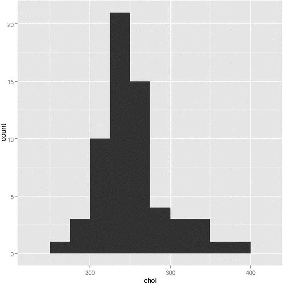
Figure 13-1. Histogram of cholesterol levels for 62 patients
With a sample size of 62, we should be able to invoke the central limit theorem and assume that the sampling distribution of means will be roughly normal. This would justify the use of a z test to compare this sample to the known mean and standard deviation of serum cholesterol levels in 20- to 74-year-old males, which are 211 and 46, respectively. To double-check the reasonability of our assumptions, we can perform a bootstrap sampling of our data to determine if the distribution of means is indeed approximately normal. See the plot of the sample means in Figure 13-2. For this plot, I converted the means to standard scores using the scale function, and then plotted the z scores with the normal curve as an overlay. Examine the following code to see how to do this. The freq = FALSE argument specifies the plotting of densities rather than frequencies, and theylim argument makes sure there is enough room on the graph for the normal curve.
nsamps <- 10000
cholMean <- numeric()
for(i in 1:nsamps) cholMean[i] <- mean(sample(chol, replace = T))
CI <- c(quantile(cholMean, 0.025), quantile(cholMean, 0.975))
CI
2.5% 97.5%
240.3867 260.6133
> zcholMean <- scale(cholMean)
> hist(zcholMean, freq = FALSE, col = "gray", ylim = c(0, 0.4))
> curve(dnorm, col = "red", add = TRUE)
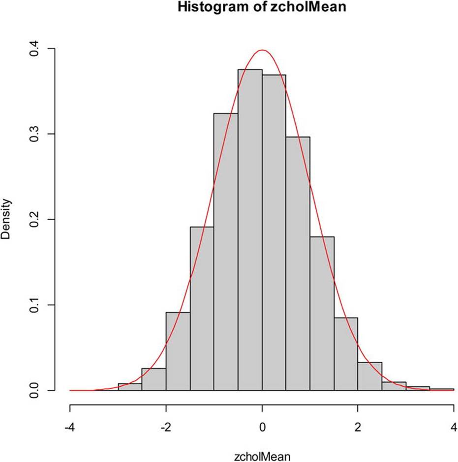
Figure 13-2. Plot of 10,000 resampled means from the cholesterol data
Let us use our modified one-sample z test function to test the null hypothesis that the sample came from a population with a mean serum cholesterol level of 211 and a standard deviation of 46 against the one-sided alternative that the sample came from a population with a higher mean cholesterol level. We will adopt an alpha level of .01 for the test.
Here is the output from the one-sample z test, followed by the output from R’s t.test function for comparison. The results are similar because the sample is relatively large.
> oneSampZ(chol, mu = 211, sigma = 46, alternative = "greater", alpha = 0.01)
one-sample z test
sample mean: 250.0645
test value: 211
sigma: 46
alternative: true mean > test value
observed z: 6.686833
p value: 1.140266e-11
99 percent confidence interval
lower: 236.474 upper: Inf
> t.test(chol,mu = 211, alternative = "greater", conf.level = 0.99)
One Sample t-test
data: chol
t = 7.429, df = 61, p-value = 2.117e-10
alternative hypothesis: true mean is greater than 211
99 percent confidence interval:
237.502 Inf
sample estimates:
mean of x
250.0645
The extremely low p values indicate we can reject the null hypothesis, and we conclude that the sample came from a population with a mean higher than 211.
For comparison’s sake, I also conducted the one-sample z test using the built-in z.test function in the BSDA package:
> library(BSDA)
> z.test(x = chol, alternative = "greater", mu = 211, sigma.x = 46, conf.level = 0.99)
One-sample z-Test
data: chol
z = 6.6868, p-value = 1.14e-11
alternative hypothesis: true mean is greater than 211
99 percent confidence interval:
236.474 NA
sample estimates:
mean of x
250.0645
Apart from labelling and the number of decimals reported, the two functions produce the same result, but BSDA used NA rather than Inf to represent the upper limit of the confidence interval.
Recipe 13-2. Writing Functions That Produce Other Functions
Problem
Recipe 13-1 shows how a function can call other R functions, such as mean and length. Many R functions are actually functions of other functions. When you create an object in a function, that object is local to the function. The last value computed in a function will be automatically returned by R, but it is often a good idea to use an explicit return() statement. To illustrate the scoping of the variables and objects in a function, note that we can define x within the function, but that assignment will not affect the value of x in the global environment (our R workspace). Similarly, R functions such as mean and length reside in the global workspace, and can be used within other functions.
The function squareX redefines x as the square of x, and then prints the new vector, but this is local to the function. When you execute the function, the values of x in the global environment are unaffected:
squareX <- function(x) {
x <- x^2
print(x)
}
> squareX(x)
[1] 8469.954 5938.378 11432.517 8755.406 8574.257 4004.169 6577.281
[8] 7978.817 3664.919 8242.086 5112.292 7149.063 7074.971 5202.297
[15] 7303.618 4876.769 5373.086 7577.157 8590.604 7122.608 9195.885
[22] 10393.261 6212.646 4804.475 9342.008 5934.501 10749.049 5390.253
[29] 6821.605 9874.911
> x
[1] 92.03235 77.06087 106.92295 93.57033 92.59728 63.27850 81.10044
[8] 89.32423 60.53857 90.78593 71.50029 84.55213 84.11285 72.12695
[15] 85.46121 69.83387 73.30134 87.04686 92.68551 84.39555 95.89518
[22] 101.94735 78.82034 69.31432 96.65406 77.03571 103.67762 73.41834
[29] 82.59301 99.37259
Functions can also produce other functions as output, which is useful in a variety of situations. For example, suppose we want to create a function that makes it easier to take various roots of numbers. R has the built-in sqrt function and the exponent operator (^), but perhaps you work with cube roots, and would rather have a function just for that.
Solution
We want to create a function called take.root, which creates a second function called root. We can use the root function to specify the desired root of a given number, as follows. We pass n to the take.root function, which then uses the root function to extract the appropriate root.
take.root <- function(n){
root <- function(x){
x^(1/n)
}
root
}
> sqrRoot <- take.root(2)
> sqrRoot(64)
[1] 8
> cubeRoot <- take.root(3)
> cubeRoot(27)
[1] 3
Observe that in our workspace, we now have functions for extracting square roots and cube roots. When you print a function without the (), R shows you the function body and the environment in which the function was created. We will discuss R environments and scoping in a little more depth in Recipe 13-3.
> ls()
[1] "chol" "cholMean" "cubeRoot" "LL" "normalDist"
[6] "oneSampZ" "repeated" "sqrRoot" "take.root" "UL"
[11] "x" "xy" "zobs"
> sqrRoot
function(x){
x^(1/n)
}
<environment: 0x0239ee44>
Recipe 13-3. Writing Functions That Request User Input
Problem
Most of the functions in R produce output that is either printed to the console or passed to some other function. Occasionally, you may want to have a function request input directly from the user. There are many ways to make R interactive, including the web application Shiny by RStudio, as we will discuss in Recipe 13-4. If your aspirations are less ambitious, you can use R functions to request user input from a function.
Solution
Assume that we are interested in obtaining user input for some of the arguments to a function. For example, what if we want a body mass index (BMI) calculator that will prompt the user for his or her height and weight? We could of course pass these as arguments to the function, but we could also ask the user to enter them after being prompted.
Here is our simple BMI function. It prompts the user for his or her height in inches and weight in pounds, and then calculates the BMI. The function also determines the person’s classification as underweight, normal, overweight, or obese, according to the standards set by the National Heart, Lung, and Blood Institute.
BMI <- function() {
cat("Please enter your height in inches and weight in pounds:","\n")
height <- as.numeric(readline("height = "))
weight <- as.numeric(readline("weight = "))
bmi <- weight/(height^2)*703
cat("Your body mass index is:",bmi,"\n")
if (bmi < 18.5) risk = "Underweight"
else if (bmi >= 18.5 && bmi <= 24.9) risk = "Normal"
else if (bmi >= 25 && bmi <= 29.9) risk = "Overweight"
else risk = "Obese"
cat("According to the National Heart, Lung, and Blood Institute,","\n")
cat("your BMI is in the",risk,"category.","\n")
}
To use the function, you simply enter BMI() at the R command prompt after copying the function into the working memory. You may recall that the function script can be saved as an R file from the R editor and loaded into the working memory by opening the script, and then selecting all the code and pressing Alt + R to “run” it. Here is how the function looks in operation. The two lines in bold are the points at which the function prompts the user for input:
> BMI()
Please enter your height in inches and weight in pounds:
height = 67
weight = 149
Your body mass index is: 23.33415
According to the National Heart, Lung, and Blood Institute,
your BMI is in the Normal category.
Recipe 13-4. Taking R to the Web
Problem
Taking R to the Web involves the use of some kind of server, whether you are running it on your local machine or using a web-based server to which you have access. RStudio makes it easy to create web applications using the Shiny package, and we will illustrate that in Recipe 13-4. Shiny is a product of Revolution Analytics, and is provided free of charge, along with the RStudio GUI for R. Many of their other value-added solutions are commercial products. Because Shiny integrates so easily with RStudio, we will illustrate Shiny with RStudio rather than the R Console.
Solution
Every Shiny application must have two scripts. One is the user interface script, and the other is the server script. The server script specifies the input and output and the user interface script specifies what the shiny application will do. For instance, Figure 13-3 shows a basic server.R script in the RStudio interface. Observe the triangle next to Run App in the code (top-left) panel. When you have Shiny installed, you will have this feature available whenever you create a Shiny application. Also notice in the right panel that shiny and shinyapps must both be installed as R packages.
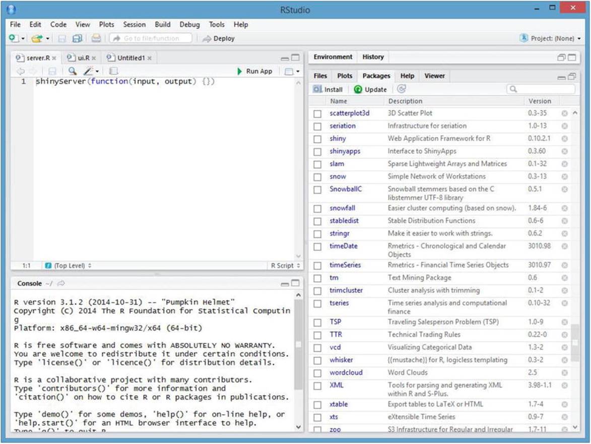
Figure 13-3. The RStudio interface with a shinyServer script in the script window
The user interface script contains the commands that make the shiny application. Here is the code for the script ui.R in my RStudio workspace (I will only show the RStudio interface if there is something new to add). One of the nice features of RStudio is that it makes sure your parentheses balance, and using indentation makes the code easier to read. See that you can use HTML-type tags in your Shiny application. Type the following and save it as ui.R:
shinyUI(fluidPage(
titlePanel("Check out Shiny"),
sidebarLayout(
sidebarPanel( "sidebar panel",
h3("Shiny is from RStudio")),
mainPanel("main panel",
h1("This is a level 1 header!")
)
))
)
Here’s what happens when you click Run App (see Figure 13-4). Note that the web application is running on my local host. If you want to look at the app in a browser, you can click Open in Browser. If you want to deploy to app to RStudio’s shiny server, you will have to register for a free account.
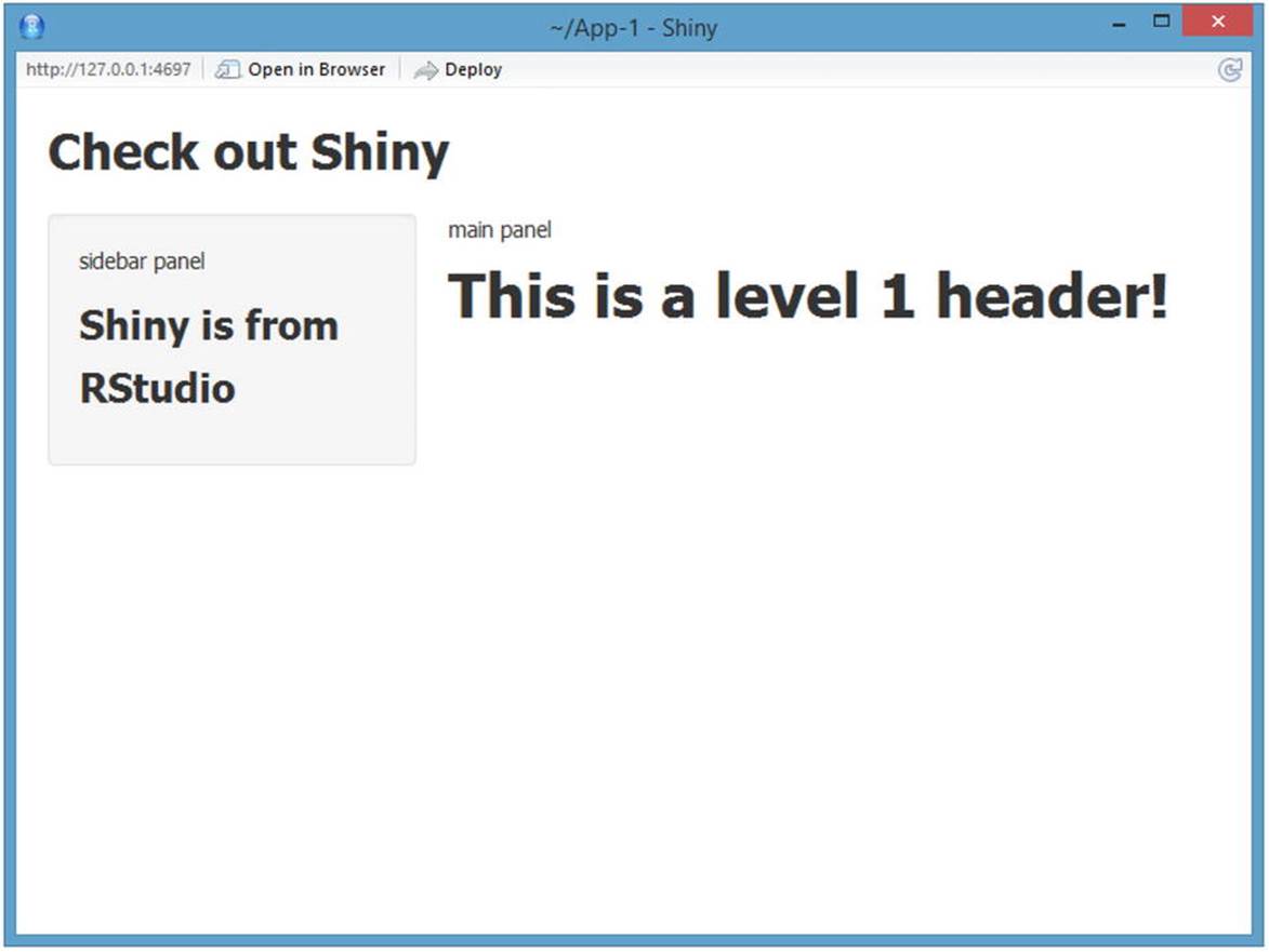
Figure 13-4. A Shiny application running in RStudio
After establishing your ShinyApps account, you can host your applications on the ShinyApps server and deploy them by clicking the Deploy button (see Figure 13-5).

Figure 13-5. Preparing to deploy a Shiny application
The application opens in a browser window with the URL https://larrypace.shinyapps.io/App-1/.
You can add interactivity to your apps very easily. For example, here is RStudio’s demonstration application of a histogram of the Old Faithful eruption data, with a slider bar for the number of bins. See that every Shiny app must have a server.R script and a ui.R script. You can display the scripts next to the output, or below it if you would rather do so (see Figure 13-6).
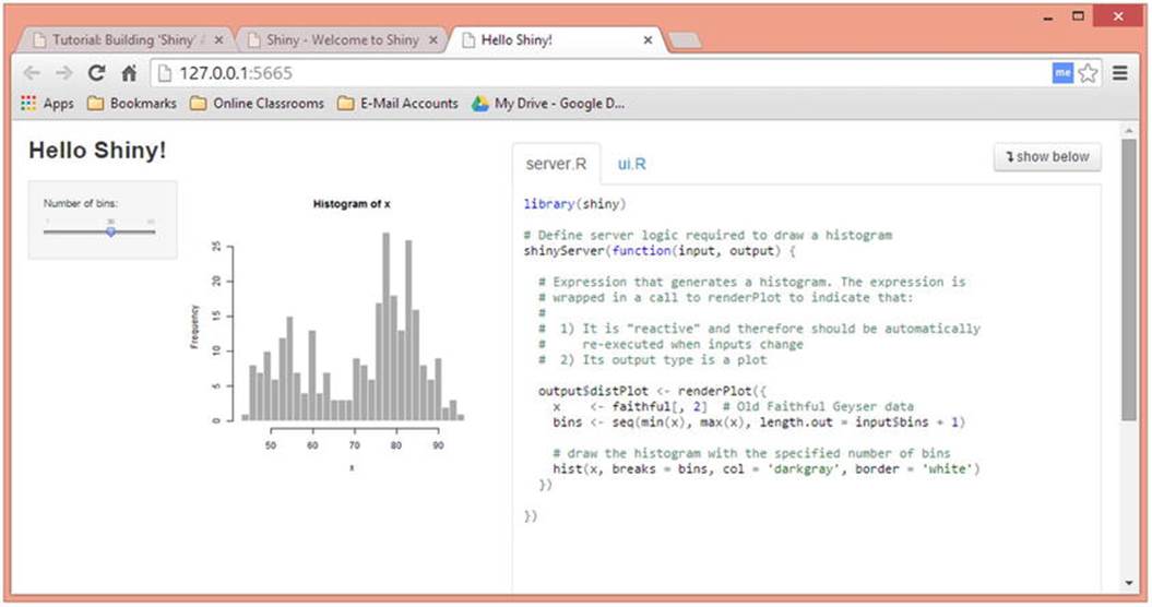
Figure 13-6. The “Hello Shiny” demonstration
Here is the ui.R script for the application:
library(shiny)
# Define UI for application that draws a histogram
shinyUI(fluidPage(
# Application title
titlePanel("Hello Shiny!"),
# Sidebar with a slider input for the number of bins
sidebarLayout(
sidebarPanel(
sliderInput("bins",
"Number of bins:",
min = 1,
max = 50,
value = 30)
),
# Show a plot of the generated distribution
mainPanel(
plotOutput("distPlot")
)
)
))
RStudio provides an excellent tutorial and a gallery of many Shiny apps that you can examine and modify. You can find these resources at http://shiny.rstudio.com. Although you do not have to be running RStudio in order to use Shiny, the two solutions play very well together, as you might expect.