Machine Learning with Spark (2015)
Chapter 3. Obtaining, Processing, and Preparing Data with Spark
Machine learning is an extremely broad field, and these days, applications can be found across areas that include web and mobile applications, Internet of Things and sensor networks, financial services, healthcare, and various scientific fields, to name just a few.
Therefore, the range of data available for potential use in machine learning is enormous. In this book, we will focus mostly on business applications. In this context, the data available often consists of data internal to an organization (such as transactional data for a financial services company) as well as external data sources (such as financial asset price data for the same financial services company).
For example, recall from Chapter 2, Designing a Machine Learning System, that the main internal source of data for our hypothetical Internet business, MovieStream, consists of data on the movies available on the site, the users of the service, and their behavior. This includes data about movies and other content (for example, title, categories, description, images, actors, and directors), user information (for example, demographics, location, and so on), and user activity data (for example, web page views, title previews and views, ratings, reviews, and social data such as likes, shares, and social network profiles on services including Facebook and Twitter).
External data sources in this example might include weather and geolocation services, third-party movie ratings and review sites such as IMDB and Rotten Tomatoes, and so on.
Generally speaking, it is quite difficult to obtain data of an internal nature for real-world services and businesses, as it is commercially sensitive (in particular, data on purchasing activity, user or customer behavior, and revenue) and of great potential value to the organization concerned. This is why it is also often the most useful and interesting data on which to apply machine learning—a good machine learning model that can make accurate predictions can be highly valuable (witness the success of machine learning competitions such as the Netflix Prize and Kaggle).
In this book, we will make use of datasets that are publicly available to illustrate concepts around data processing and training of machine learning models.
In this chapter, we will:
· Briefly cover the types of data typically used in machine learning.
· Provide examples of where to obtain interesting datasets, often publicly available on the Internet. We will use some of these datasets throughout the book to illustrate the use of the models we introduce.
· Discover how to process, clean, explore, and visualize our data.
· Introduce various techniques to transform our raw data into features that can be used as input to machine learning algorithms.
· Learn how to normalize input features using external libraries as well as Spark's built-in functionality.
Accessing publicly available datasets
Fortunately, while commercially-sensitive data can be hard to come by, there are still a number of useful datasets available publicly. Many of these are often used as benchmark datasets for specific types of machine learning problems. Examples of common data sources include:
· UCI Machine Learning Repository: This is a collection of almost 300 datasets of various types and sizes for tasks including classification, regression, clustering, and recommender systems. The list is available at http://archive.ics.uci.edu/ml/.
· Amazon AWS public datasets: This is a set of often very large datasets that can be accessed via Amazon S3. These datasets include the Human Genome Project, the Common Crawl web corpus, Wikipedia data, and Google Books Ngrams. Information on these datasets can be found at http://aws.amazon.com/publicdatasets/.
· Kaggle: This is a collection of datasets used in machine learning competitions run by Kaggle. Areas include classification, regression, ranking, recommender systems, and image analysis. These datasets can be found under the Competitions section athttp://www.kaggle.com/competitions.
· KDnuggets: This has a detailed list of public datasets, including some of those mentioned earlier. The list is available at http://www.kdnuggets.com/datasets/index.html.
Tip
There are many other resources to find public datasets depending on the specific domain and machine learning task. Hopefully, you might also have exposure to some interesting academic or commercial data of your own!
To illustrate a few key concepts related to data processing, transformation, and feature extraction in Spark, we will download a commonly-used dataset for movie recommendations; this dataset is known as the MovieLens dataset. As it is applicable to recommender systems as well as potentially other machine learning tasks, it serves as a useful example dataset.
Note
Spark's machine learning library, MLlib, has been under heavy development since its inception, and unlike the Spark core, it is still not in a fully stable state with regard to its overall API and design.
As of Spark Version 1.2.0, a new, experimental API for MLlib has been released under the ml package (whereas the current library resides under the mllib package). This new API aims to enhance the APIs and interfaces for models as well as feature extraction and transformation so as to make it easier to build pipelines that chain together steps that include feature extraction, normalization, dataset transformations, model training, and cross-validation.
In the upcoming chapters, we will only cover the existing, more developed MLlib API, since the new API is still experimental and may be subject to major changes in the next few Spark releases. Over time, the various feature-processing techniques and models that we will cover will simply be ported to the new API; however, the core concepts and most underlying code will remain largely unchanged.
The MovieLens 100k dataset
The MovieLens 100k dataset is a set of 100,000 data points related to ratings given by a set of users to a set of movies. It also contains movie metadata and user profiles. While it is a small dataset, you can quickly download it and run Spark code on it. This makes it ideal for illustrative purposes.
You can download the dataset from http://files.grouplens.org/datasets/movielens/ml-100k.zip.
Once you have downloaded the data, unzip it using your terminal:
>unzip ml-100k.zip
inflating: ml-100k/allbut.pl
inflating: ml-100k/mku.sh
inflating: ml-100k/README
...
inflating: ml-100k/ub.base
inflating: ml-100k/ub.test
This will create a directory called ml-100k. Change into this directory and examine the contents. The important files are u.user (user profiles), u.item (movie metadata), and u.data (the ratings given by users to movies):
>cd ml-100k
The README file contains more information on the dataset, including the variables present in each data file. We can use the head command to examine the contents of the various files.
For example, we can see that the u.user file contains the user id, age, gender, occupation, and ZIP code fields, separated by a pipe (| character):
>head -5 u.user
1|24|M|technician|85711
2|53|F|other|94043
3|23|M|writer|32067
4|24|M|technician|43537
5|33|F|other|15213
The u.item file contains the movie id, title, release data, and IMDB link fields and a set of fields related to movie category data. It is also separated by a | character:
>head -5 u.item
1|Toy Story (1995)|01-Jan-1995||http://us.imdb.com/M/title-exact?Toy%20Story%20(1995)|0|0|0|1|1|1|0|0|0|0|0|0|0|0|0|0|0|0|0
2|GoldenEye (1995)|01-Jan-1995||http://us.imdb.com/M/title-exact?GoldenEye%20(1995)|0|1|1|0|0|0|0|0|0|0|0|0|0|0|0|0|1|0|0
3|Four Rooms (1995)|01-Jan-1995||http://us.imdb.com/M/title-exact?Four%20Rooms%20(1995)|0|0|0|0|0|0|0|0|0|0|0|0|0|0|0|0|1|0|0
4|Get Shorty (1995)|01-Jan-1995||http://us.imdb.com/M/title-exact?Get%20Shorty%20(1995)|0|1|0|0|0|1|0|0|1|0|0|0|0|0|0|0|0|0|0
5|Copycat (1995)|01-Jan-1995||http://us.imdb.com/M/title-exact?Copycat%20(1995)|0|0|0|0|0|0|1|0|1|0|0|0|0|0|0|0|1|0|0
Finally, the u.data file contains the user id, movie id, rating (1-5 scale), and timestamp fields and is separated by a tab (the \t character):
>head -5 u.data
196 242 3 881250949
186 302 3 891717742
22 377 1 878887116
244 51 2 880606923
166 346 1 886397596
Exploring and visualizing your data
Now that we have our data available, let's fire up an interactive Spark console and explore it! For this section, we will use Python and the PySpark shell, as we are going to use the IPython interactive console and the matplotlib plotting library to process and visualize our data.
Note
IPython is an advanced, interactive shell for Python. It includes a useful set of features called pylab, which includes NumPy and SciPy for numerical computing and matplotlib for interactive plotting and visualization.
We recommend that you use the latest version of IPython (2.3.1 at the time of writing this book). To install IPython for your platform, follow the instructions available at http://ipython.org/install.html. If this is the first time you are using IPython, you can find a tutorial at http://ipython.org/ipython-doc/stable/interactive/tutorial.html.
You will need to install all the packages listed earlier in order to work through the code in this chapter. Instructions to install the packages can be found in the code bundle. If you are starting out with Python or are unfamiliar with the process of installing these packages, we strongly recommend that you use a prebuilt scientific Python installation such as Anaconda (available at http://continuum.io/downloads) or Enthought (available at https://store.enthought.com/downloads/). These make the installation process much easier and include everything you will need to follow the example code.
The PySpark console allows the option of setting which Python executable needs to be used to run the shell. We can choose to use IPython, as opposed to the standard Python shell, when launching our PySpark console. We can also pass in additional options to IPython, including telling it to launch with the pylab functionality enabled.
We can do this by running the following command from the Spark home directory (that is, the same directory that we used previously to explore the Spark interactive console):
>IPYTHON=1 IPYTHON_OPTS="--pylab" ./bin/pyspark
You will see the PySpark console start up, showing output similar to the following screenshot:
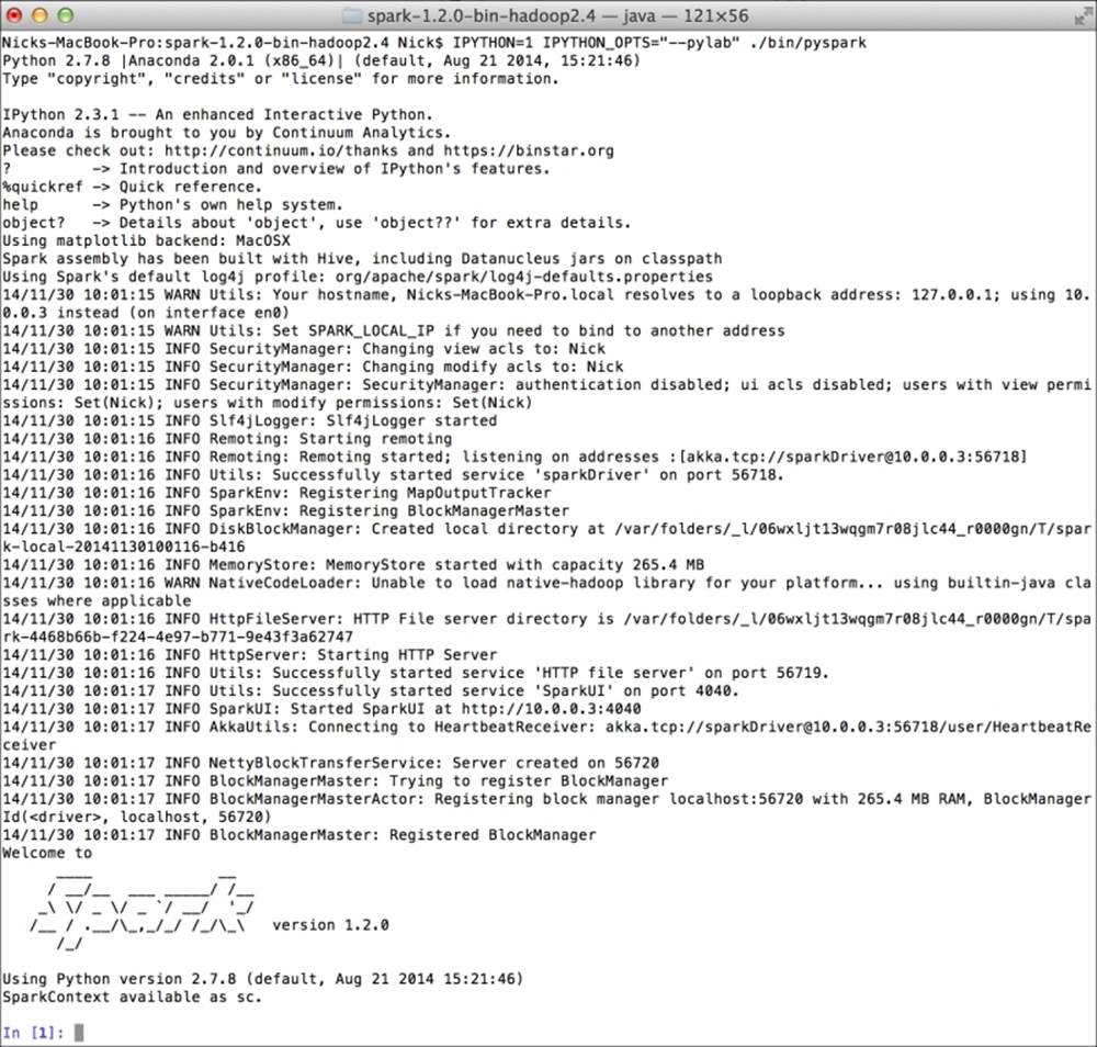
The PySpark console using IPython
Tip
Notice the IPython 2.3.1 -- An enhanced Interactive Python and Using matplotlib backend: MacOSX lines; they indicate that both the IPython and pylab functionalities are being used by the PySpark shell.
You might see a slightly different output, depending on your operating system and software versions.
Now that we have our IPython console open, we can start to explore the MovieLens dataset and do some basic analysis.
Note
You can follow along with this chapter by entering the code examples into your IPython console. IPython also provides an HTML-enabled Notebook application. It provides some enhanced functionality over the standard IPython console, such as inline graphics for plotting, the HTML markup functionality, as well as the ability to run cells of code independently.
The images used in this chapter were generated using the IPython Notebook, so don't worry if yours look a little bit different in style, as long as they contain the same content! You can also use the Notebook for the code in this chapter, if you prefer. In addition to the Python code for this chapter, we have provided a version saved in the IPython Notebook format, which you can load into your own IPython Notebook.
Check out the instructions on how to use the IPython Notebook at http://ipython.org/ipython-doc/stable/interactive/notebook.html.
Exploring the user dataset
First, we will analyze the characteristics of MovieLens users. Enter the following lines into your console (where PATH refers to the base directory in which you performed the unzip command to unzip the preceding MovieLens 100k dataset):
user_data = sc.textFile("/PATH/ml-100k/u.user")
user_data.first()
You should see output similar to this:
u'1|24|M|technician|85711'
As we can see, this is the first line of our user data file, separated by the "|" character.
Tip
The first function is similar to collect, but it only returns the first element of the RDD to the driver. We can also use take(k) to collect only the first k elements of the RDD to the driver.
Let's transform the data by splitting each line, around the "|" character. This will give us an RDD where each record is a Python list that contains the user ID, age, gender, occupation, and ZIP code fields.
We will then count the number of users, genders, occupations, and ZIP codes. We can achieve this by running the following code in the console, line by line. Note that we do not cache the data, as it is unnecessary for this small size:
user_fields = user_data.map(lambda line: line.split("|"))
num_users = user_fields.map(lambda fields: fields[0]).count()
num_genders = user_fields.map(lambda fields:fields[2]).distinct().count()
num_occupations = user_fields.map(lambda fields:fields[3]).distinct().count()
num_zipcodes = user_fields.map(lambda fields:fields[4]).distinct().count()
print "Users: %d, genders: %d, occupations: %d, ZIP codes: %d" % (num_users, num_genders, num_occupations, num_zipcodes)
You will see the following output:
Users: 943, genders: 2, occupations: 21, ZIP codes: 795
Next, we will create a histogram to analyze the distribution of user ages, using matplotlib's hist function:
ages = user_fields.map(lambda x: int(x[1])).collect()
hist(ages, bins=20, color='lightblue', normed=True)
fig = matplotlib.pyplot.gcf()
fig.set_size_inches(16, 10)
We passed in the ages array, together with the number of bins for our histogram (20 in this case), to the hist function. Using the normed=True argument, we also specified that we want the histogram to be normalized so that each bucket represents the percentage of the overall data that falls into that bucket.
You will see an image containing the histogram chart, which looks something like the one shown here. As we can see, the ages of MovieLens users are somewhat skewed towards younger viewers. A large number of users are between the ages of about 15 and 35.
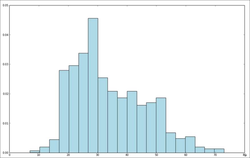
Distribution of user ages
We might also want to explore the relative frequencies of the various occupations of our users. We can do this using the following code snippet. First, we will use the MapReduce approach introduced previously to count the occurrences of each occupation in the dataset. Then, we will use matplotlib to display a bar chart of occupation counts, using the bar function.
Since part of our data is the descriptions of textual occupation, we will need to manipulate it a little to get it to work with the bar function:
count_by_occupation = user_fields.map(lambda fields: (fields[3], 1)).reduceByKey(lambda x, y: x + y).collect()
x_axis1 = np.array([c[0] for c in count_by_occupation])
y_axis1 = np.array([c[1] for c in count_by_occupation])
Once we have collected the RDD of counts per occupation, we will convert it into two arrays for the x axis (the occupations) and the y axis (the counts) of our chart. The collect function returns the count data to us in no particular order. We need to sort the count data so that our bar chart is ordered from the lowest to the highest count.
We will achieve this by first creating two numpy arrays and then using the argsort method of numpy to select the elements from each array, ordered by the count data in an ascending fashion. Notice that here, we will sort both the x and y axis arrays by the y axis (that is, by the counts):
x_axis = x_axis1[np.argsort(y_axis1)]
y_axis = y_axis1[np.argsort(y_axis1)]
Once we have the x and y axis data for our chart, we will create the bar chart with the occupations as labels on the x axis and the counts as the values on the y axis. We will also add a few lines, such as the plt.xticks(rotation=30) code, to display a better-looking chart:
pos = np.arange(len(x_axis))
width = 1.0
ax = plt.axes()
ax.set_xticks(pos + (width / 2))
ax.set_xticklabels(x_axis)
plt.bar(pos, y_axis, width, color='lightblue')
plt.xticks(rotation=30)
fig = matplotlib.pyplot.gcf()
fig.set_size_inches(16, 10)
The image you have generated should look like the one here. It appears that the most prevalent occupations are student, other, educator, administrator, engineer, and programmer.
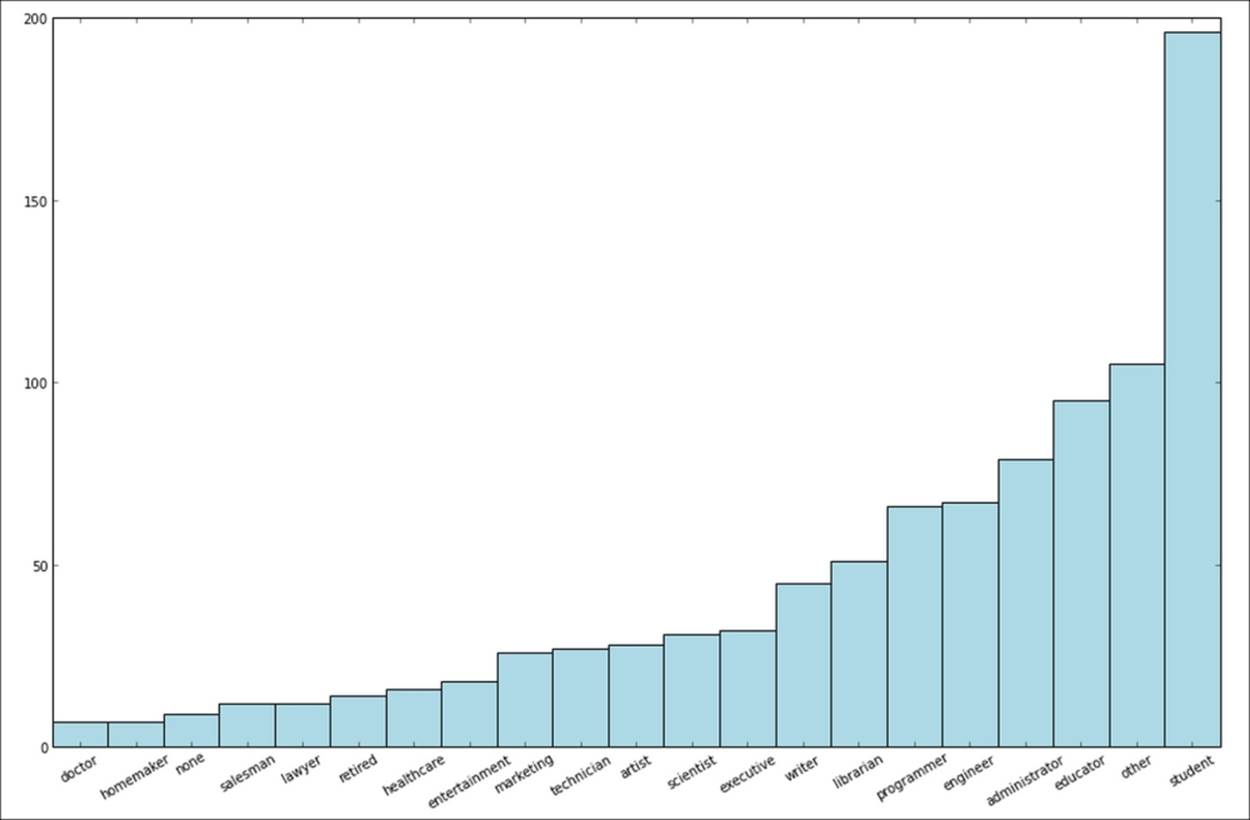
Distribution of user occupations
Spark provides a convenience method on RDDs called countByValue; this method counts the occurrences of each unique value in the RDD and returns it to the driver as a Python dict method (or a Scala or Java Map method). We can create the count_by_occupationvariable using this method:
count_by_occupation2 = user_fields.map(lambda fields: fields[3]).countByValue()
print "Map-reduce approach:"
print dict(count_by_occupation2)
print ""
print "countByValue approach:"
print dict(count_by_occupation)
You should see that the results are the same for each approach.
Exploring the movie dataset
Next, we will investigate a few properties of the movie catalogue. We can inspect a row of the movie data file, as we did for the user data earlier, and then count the number of movies:
movie_data = sc.textFile("/PATH/ml-100k/u.item")
print movie_data.first()
num_movies = movie_data.count()
print "Movies: %d" % num_movies
You will see the following output on your console:
1|Toy Story (1995)|01-Jan-1995||http://us.imdb.com/M/title-exact?Toy%20Story%20(1995)|0|0|0|1|1|1|0|0|0|0|0|0|0|0|0|0|0|0|0
Movies: 1682
In the same manner as we did for user ages and occupations earlier, we can plot the distribution of movie age, that is, the year of release relative to the current date (note that for this dataset, the current year is 1998).
In the following code block, we can see that we need a small function called convert_year to handle errors in the parsing of the release date field. This is due to some bad data in one line of the movie data:
def convert_year(x):
try:
return int(x[-4:])
except:
return 1900 # there is a 'bad' data point with a blank year,
which we set to 1900 and will filter out later
Once we have our utility function to parse the year of release, we can apply it to the movie data using a map transformation and collect the results:
movie_fields = movie_data.map(lambda lines: lines.split("|"))
years = movie_fields.map(lambda fields: fields[2]).map(lambda x: convert_year(x))
Since we have assigned the value 1900 to any error in parsing, we can filter these bad values out of the resulting data using Spark's filter transformation:
years_filtered = years.filter(lambda x: x != 1900)
This is a good example of how real-world datasets can often be messy and require a more in-depth approach to parsing data. In fact, this also illustrates why data exploration is so important, as many of these issues in data integrity and quality are picked up during this phase.
After filtering out bad data, we will transform the list of movie release years into movie ages by subtracting the current year, use countByValue to compute the counts for each movie age, and finally, plot our histogram of movie ages (again, using the hist function, where the values variable are the values of the result from countByValue, and the bins variable are the keys):
movie_ages = years_filtered.map(lambda yr: 1998-yr).countByValue()
values = movie_ages.values()
bins = movie_ages.keys()
hist(values, bins=bins, color='lightblue', normed=True)
fig = matplotlib.pyplot.gcf()
fig.set_size_inches(16,10)
You will see an image similar to the one here; it illustrates that most of the movies were released in the last few years before 1998:
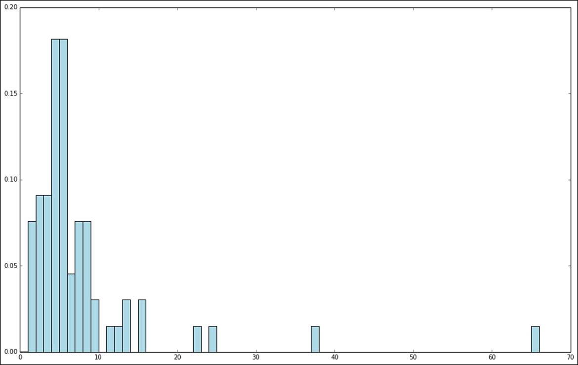
Distribution of movie ages
Exploring the rating dataset
Let's now take a look at the ratings data:
rating_data = sc.textFile("/PATH/ml-100k/u.data")
print rating_data.first()
num_ratings = rating_data.count()
print "Ratings: %d" % num_ratings
This gives us the following result:
196 242 3 881250949
Ratings: 100000
There are 100,000 ratings, and unlike the user and movie datasets, these records are split with a tab character ("\t"). As you might have guessed, we'd probably want to compute some basic summary statistics and frequency histograms for the rating values. Let's do this now:
rating_data = rating_data_raw.map(lambda line: line.split("\t"))
ratings = rating_data.map(lambda fields: int(fields[2]))
max_rating = ratings.reduce(lambda x, y: max(x, y))
min_rating = ratings.reduce(lambda x, y: min(x, y))
mean_rating = ratings.reduce(lambda x, y: x + y) / num_ratings
median_rating = np.median(ratings.collect())
ratings_per_user = num_ratings / num_users
ratings_per_movie = num_ratings / num_movies
print "Min rating: %d" % min_rating
print "Max rating: %d" % max_rating
print "Average rating: %2.2f" % mean_rating
print "Median rating: %d" % median_rating
print "Average # of ratings per user: %2.2f" % ratings_per_user
print "Average # of ratings per movie: %2.2f" % ratings_per_movie
After running these lines on your console, you will see output similar to the following result:
Min rating: 1
Max rating: 5
Average rating: 3.53
Median rating: 4
Average # of ratings per user: 106.00
Average # of ratings per movie: 59.00
We can see that the minimum rating is 1, while the maximum rating is 5. This is in line with what we expect, since the ratings are on a scale of 1 to 5.
Spark also provides a stats function for RDDs; this function contains a numeric variable (such as ratings in this case) to compute similar summary statistics:
ratings.stats()
Here is the output:
(count: 100000, mean: 3.52986, stdev: 1.12566797076, max: 5.0, min: 1.0)
Looking at the results, the average rating given by a user to a movie is around 3.5 and the median rating is 4, so we might expect that the distribution of ratings will be skewed towards slightly higher ratings. Let's see whether this is true by creating a bar chart of rating values using a similar procedure as we did for occupations:
count_by_rating = ratings.countByValue()
x_axis = np.array(count_by_rating.keys())
y_axis = np.array([float(c) for c in count_by_rating.values()])
# we normalize the y-axis here to percentages
y_axis_normed = y_axis / y_axis.sum()
pos = np.arange(len(x_axis))
width = 1.0
ax = plt.axes()
ax.set_xticks(pos + (width / 2))
ax.set_xticklabels(x_axis)
plt.bar(pos, y_axis_normed, width, color='lightblue')
plt.xticks(rotation=30)
fig = matplotlib.pyplot.gcf()
fig.set_size_inches(16, 10)
The preceding code should produce the following chart:
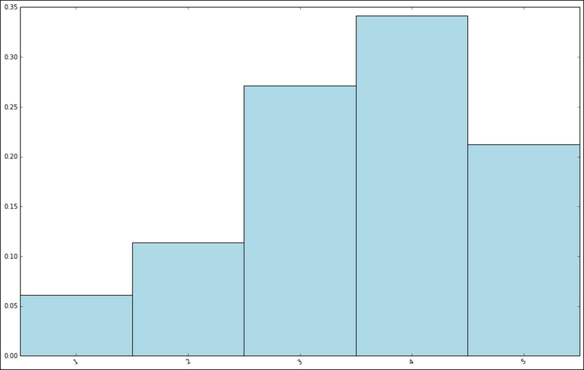
Distribution of rating values
In line with what we might have expected after seeing some summary statistics, it is clear that the distribution of ratings is skewed towards average to high ratings.
We can also look at the distribution of the number of ratings made by each user. Recall that we previously computed the rating_data RDD used in the preceding code by splitting the ratings with the tab character. We will now use the rating_data variable again in the following code.
To compute the distribution of ratings per user, we will first extract the user ID as key and rating as value from rating_data RDD. We will then group the ratings by user ID using Spark's groupByKey function:
user_ratings_grouped = rating_data.map(lambda fields: (int(fields[0]), int(fields[2]))).\
groupByKey()
Next, for each key (user ID), we will find the size of the set of ratings; this will give us the number of ratings for that user:
user_ratings_byuser = user_ratings_grouped.map(lambda (k, v): (k, len(v)))
user_ratings_byuser.take(5)
We can inspect the resulting RDD by taking a few records from it; this should give us an RDD of the (user ID, number of ratings) pairs:
[(1, 272), (2, 62), (3, 54), (4, 24), (5, 175)]
Finally, we will plot the histogram of number of ratings per user using our favorite hist function:
user_ratings_byuser_local = user_ratings_byuser.map(lambda (k, v):v).collect()
hist(user_ratings_byuser_local, bins=200, color='lightblue',normed=True)
fig = matplotlib.pyplot.gcf()
fig.set_size_inches(16,10)
Your chart should look similar to the following screenshot. We can see that most of the users give fewer than 100 ratings. The distribution of the ratings shows, however, that there are fairly large number of users that provide hundreds of ratings.
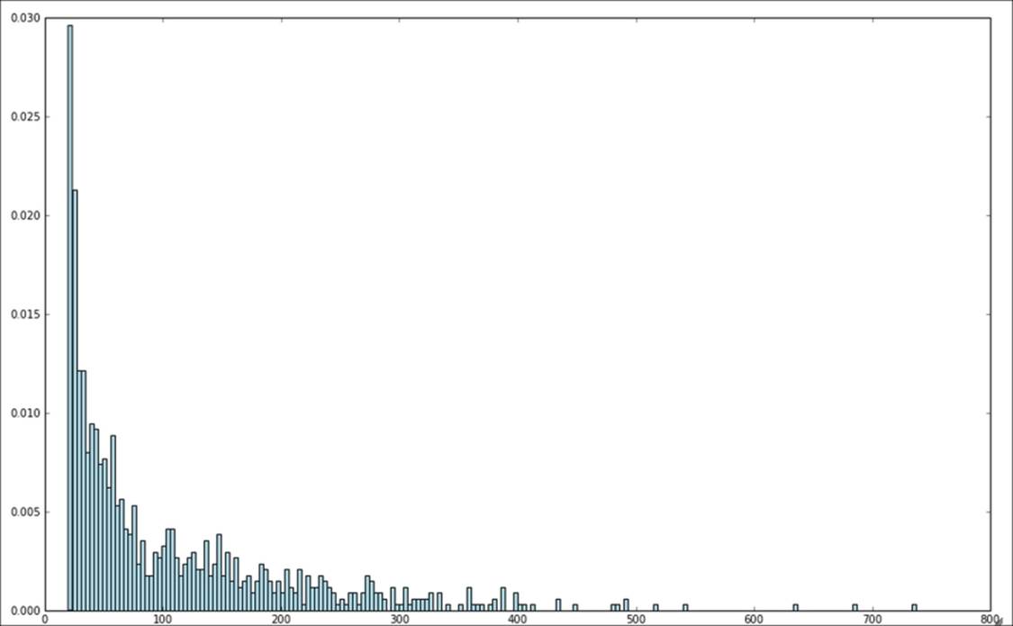
Distribution of ratings per user
We leave it to you to perform a similar analysis to create a histogram plot for the number of ratings given to each movie. Perhaps, if you're feeling adventurous, you could also extract a dataset of movie ratings by date (taken from the timestamps in the last column of the rating dataset) and chart a time series of the total number of ratings, number of unique users who gave a rating, and the number of unique movies rated, for each day.
Processing and transforming your data
Now that we have done some initial exploratory analysis of our dataset and we know a little more about the characteristics of our users and movies, what do we do next?
In order to make the raw data usable in a machine learning algorithm, we first need to clean it up and possibly transform it in various ways before extracting useful features from the transformed data. The transformation and feature extraction steps are closely linked, and in some cases, certain transformations are themselves a case of feature extraction.
We have already seen an example of the need to clean data in the movie dataset. Generally, real-world datasets contain bad data, missing data points, and outliers. Ideally, we would correct bad data; however, this is often not possible, as many datasets derive from some form of collection process that cannot be repeated (this is the case, for example, in web activity data and sensor data). Missing values and outliers are also common and can be dealt with in a manner similar to bad data. Overall, the broad options are as follows:
· Filter out or remove records with bad or missing values: This is sometimes unavoidable; however, this means losing the good part of a bad or missing record.
· Fill in bad or missing data: We can try to assign a value to bad or missing data based on the rest of the data we have available. Approaches can include assigning a zero value, assigning the global mean or median, interpolating nearby or similar data points (usually, in a time-series dataset), and so on. Deciding on the correct approach is often a tricky task and depends on the data, situation, and one's own experience.
· Apply robust techniques to outliers: The main issue with outliers is that they might be correct values, even though they are extreme. They might also be errors. It is often very difficult to know which case you are dealing with. Outliers can also be removed or filled in, although fortunately, there are statistical techniques (such as robust regression) to handle outliers and extreme values.
· Apply transformations to potential outliers: Another approach for outliers or extreme values is to apply transformations, such as a logarithmic or Gaussian kernel transformation, to features that have potential outliers, or display large ranges of potential values. These types of transformations have the effect of dampening the impact of large changes in the scale of a variable and turning a nonlinear relationship into one that is linear.
Filling in bad or missing data
We have already seen an example of filtering out bad data. Following on from the preceding code, the following code snippet applies the fill-in approach to the bad release date record by assigning a value to the data point that is equal to the median year of release:
years_pre_processed = movie_fields.map(lambda fields: fields[2]).map(lambda x: convert_year(x)).collect()
years_pre_processed_array = np.array(years_pre_processed)
First, we will compute the mean and median year of release after selecting all the year of release data, except the bad data point. We will then use the numpy function, where, to find the index of the bad value in years_pre_processed_array (recall that we assigned the value 1900 to this data point). Finally, we will use this index to assign the median release year to the bad value:
mean_year = np.mean(years_pre_processed_array[years_pre_processed_array!=1900])
median_year = np.median(years_pre_processed_array[years_pre_processed_array!=1900])
index_bad_data = np.where(years_pre_processed_array==1900)[0][0]
years_pre_processed_array[index_bad_data] = median_year
print "Mean year of release: %d" % mean_year
print "Median year of release: %d" % median_year
print "Index of '1900' after assigning median: %s" % np.where(years_pre_processed_array == 1900)[0]
You should expect to see the following output:
Mean year of release: 1989
Median year of release: 1995
Index of '1900' after assigning median: []
We computed both the mean and the median year of release here. As can be seen from the output, the median release year is quite higher because of the skewed distribution of the years. While it is not always straightforward to decide on precisely which fill-in value to use for a given situation, in this case, it is certainly feasible to use the median due to this skew.
Tip
Note that the preceding code example is, strictly speaking, not very scalable, as it requires collecting all the data to the driver. We can use Spark's mean function for numeric RDDs to compute the mean, but there is no median function available currently. We can solve this by creating our own or by computing the median on a sample of the dataset created using the sample function (we will see more of this in the upcoming chapters).
Extracting useful features from your data
Once we have completed the initial exploration, processing, and cleaning of our data, we are ready to get down to the business of extracting actual features from the data, with which our machine learning model can be trained.
Features refer to the variables that we use to train our model. Each row of data contains various information that we would like to extract into a training example. Almost all machine learning models ultimately work on numerical representations in the form of avector; hence, we need to convert raw data into numbers.
Features broadly fall into a few categories, which are as follows:
· Numerical features: These features are typically real or integer numbers, for example, the user age that we used in an example earlier.
· Categorical features: These features refer to variables that can take one of a set of possible states at any given time. Examples from our dataset might include a user's gender or occupation or movie categories.
· Text features: These are features derived from the text content in the data, for example, movie titles, descriptions, or reviews.
· Other features: Most other types of features are ultimately represented numerically. For example, images, video, and audio can be represented as sets of numerical data. Geographical locations can be represented as latitude and longitude or geohash data.
Here we will cover numerical, categorical, and text features.
Numerical features
What is the difference between any old number and a numerical feature? Well, in reality, any numerical data can be used as an input variable. However, in a machine learning model, we learn about a vector of weights for each feature. The weights play a role in mapping feature values to an outcome or target variable (in the case of supervised learning models).
Thus, we want to use features that make sense, that is, where the model can learn the relationship between feature values and the target variable. For example, age might be a reasonable feature. Perhaps there is a direct relationship between increasing age and a certain outcome. Similarly, height is a good example of a numerical feature that can be used directly.
We will often see that numerical features are less useful in their raw form, but can be turned into representations that are more useful. Location is an example of such a case. Using raw locations (say, latitude and longitude) might not be that useful unless our data is very dense indeed, since our model might not be able to learn about a useful relationship between the raw location and an outcome. However, a relationship might exist between some aggregated or binned representation of the location (for example, a city or country) and the outcome.
Categorical features
Categorical features cannot be used as input in their raw form, as they are not numbers; instead, they are members of a set of possible values that the variable can take. In the example mentioned earlier, user occupation is a categorical variable that can take the value of student, programmer, and so on.
Such categorical variables are also known as nominal variables where there is no concept of order between the values of the variable. By contrast, when there is a concept of order between variables (such as the ratings mentioned earlier, where a rating of 5 is conceptually higher or better than a rating of 1), we refer to ordinal variables.
To transform categorical variables into a numerical representation, we can use a common approach known as 1-of-k encoding. An approach such as 1-of-k encoding is required to represent nominal variables in a way that makes sense for machine learning tasks. Ordinal variables might be used in their raw form but are often encoded in the same way as nominal variables.
Assume that there are k possible values that the variable can take. If we assign each possible value an index from the set of 1 to k, then we can represent a given state of the variable using a binary vector of length k; here, all entries are zero, except the entry at the index that corresponds to the given state of the variable. This entry is set to one.
For example, we can collect all the possible states of the occupation variable:
all_occupations = user_fields.map(lambda fields: fields[3]).distinct().collect()
all_occupations.sort()
We can then assign index values to each possible occupation in turn (note that we start from zero, since Python, Scala, and Java arrays all use zero-based indices):
idx = 0
all_occupations_dict = {}
for o in all_occupations:
all_occupations_dict[o] = idx
idx +=1
# try a few examples to see what "1-of-k" encoding is assigned
print "Encoding of 'doctor': %d" % all_occupations_dict['doctor']
print "Encoding of 'programmer': %d" % all_occupations_dict['programmer']
You will see the following output:
Encoding of 'doctor': 2
Encoding of 'programmer': 14
Finally, we can encode the value of programmer. We will start by creating a numpy array of a length that is equal to the number of possible occupations (k in this case) and filling it with zeros. We will use the zeros function of numpy to create this array.
We will then extract the index of the word programmer and assign a value of 1 to the array value at this index:
K = len(all_occupations_dict)
binary_x = np.zeros(K)
k_programmer = all_occupations_dict['programmer']
binary_x[k_programmer] = 1
print "Binary feature vector: %s" % binary_x
print "Length of binary vector: %d" % K
This will give us the resulting binary feature vector of length 21:
Binary feature vector: [ 0. 0. 0. 0. 0. 0. 0. 0. 0. 0. 0. 0. 0. 0. 1. 0. 0. 0. 0. 0. 0.]
Length of binary vector: 21
Derived features
As we mentioned earlier, it is often useful to compute a derived feature from one or more available variables. We hope that the derived feature can add more information than only using the variable in its raw form.
For instance, we can compute the average rating given by each user to all the movies they rated. This would be a feature that could provide a user-specific intercept in our model (in fact, this is a commonly used approach in recommendation models). We have taken the raw rating data and created a new feature that can allow us to learn a better model.
Examples of features derived from raw data include computing average values, median values, variances, sums, differences, maximums or minimums, and counts. We have already seen a case of this when we created a new movie age feature from the year of release of the movie and the current year. Often, the idea behind using these transformations is to summarize the numerical data in some way that might make it easier for a model to learn.
It is also common to transform numerical features into categorical features, for example, by binning features. Common examples of this include variables such as age, geolocation, and time.
Transforming timestamps into categorical features
To illustrate how to derive categorical features from numerical data, we will use the times of the ratings given by users to movies. These are in the form of Unix timestamps. We can use Python's datetime module to extract the date and time from the timestamp and, in turn, extract the hour of the day. This will result in an RDD of the hour of the day for each rating.
We will need a function to extract a datetime representation of the rating timestamp (in seconds); we will create this function now:
def extract_datetime(ts):
import datetime
return datetime.datetime.fromtimestamp(ts)
We will again use the rating_data RDD that we computed in the earlier examples as our starting point.
First, we will use a map transformation to extract the timestamp field, converting it to a Python int datatype. We will then apply our extract_datetime function to each timestamp and extract the hour from the resulting datetime object:
timestamps = rating_data.map(lambda fields: int(fields[3]))
hour_of_day = timestamps.map(lambda ts: extract_datetime(ts).hour)
hour_of_day.take(5)
If we take the first five records of the resulting RDD, we will see the following output:
[17, 21, 9, 7, 7]
We have transformed the raw time data into a categorical feature that represents the hour of the day in which the rating was given.
Now, say that we decide this is too coarse a representation. Perhaps we want to further refine the transformation. We can assign each hour-of-the-day value into a defined bucket that represents a time of day.
For example, we can say that morning is from 7 a.m. to 11 a.m., while lunch is from 11 a.m. to 1 a.m., and so on. Using these buckets, we can create a function to assign a time of day, given the hour of the day as input:
def assign_tod(hr):
times_of_day = {
'morning' : range(7, 12),
'lunch' : range(12, 14),
'afternoon' : range(14, 18),
'evening' : range(18, 23),
'night' : range(23, 7)
}
for k, v in times_of_day.iteritems():
if hr in v:
return k
Now, we will apply the assign_tod function to the hour of each rating event contained in the hour_of_day RDD:
time_of_day = hour_of_day.map(lambda hr: assign_tod(hr))
time_of_day.take(5)
If we again take the first five records of this new RDD, we will see the following transformed values:
['afternoon', 'evening', 'morning', 'morning', 'morning']
We have now transformed the timestamp variable (which can take on thousands of values and is probably not useful to a model in its raw form) into hours (taking on 24 values) and then into a time of day (taking on five possible values). Now that we have a categorical feature, we can use the same 1-of-k encoding method outlined earlier to generate a binary feature vector.
Text features
In some ways, text features are a form of categorical and derived features. Let's take the example of the description for a movie (which we do not have in our dataset). Here, the raw text could not be used directly, even as a categorical feature, since there are virtually unlimited possible combinations of words that could occur if each piece of text was a possible value. Our model would almost never see two occurrences of the same feature and would not be able to learn effectively. Therefore, we would like to turn raw text into a form that is more amenable to machine learning.
There are numerous ways of dealing with text, and the field of natural language processing is dedicated to processing, representing, and modeling textual content. A full treatment is beyond the scope of this book, but we will introduce a simple and standard approach for text-feature extraction; this approach is known as the bag-of-words representation.
The bag-of-words approach treats a piece of text content as a set of the words, and possibly numbers, in the text (these are often referred to as terms). The process of the bag-of-words approach is as follows:
· Tokenization: First, some form of tokenization is applied to the text to split it into a set of tokens (generally words, numbers, and so on). An example of this is simple whitespace tokenization, which splits the text on each space and might remove punctuation and other characters that are not alphabetical or numerical.
· Stop word removal: Next, it is usual to remove very common words such as "the", "and", and "but" (these are known as stop words).
· Stemming: The next step can include stemming, which refers to taking a term and reducing it to its base form or stem. A common example is plural terms becoming singular (for example, dogs becomes dog and so on). There are many approaches to stemming, and text-processing libraries often contain various stemming algorithms.
· Vectorization: The final step is turning the processed terms into a vector representation. The simplest form is, perhaps, a binary vector representation, where we assign a value of one if a term exists in the text and zero if it does not. This is essentially identical to the categorical 1-of-k encoding we encountered earlier. Like 1-of-k encoding, this requires a dictionary of terms mapping a given term to an index number. As you might gather, there are potentially millions of individual possible terms (even after stop word removal and stemming). Hence, it becomes critical to use a sparse vector representation where only the fact that a term is present is stored, to save memory and disk space as well as compute time.
Note
In Chapter 9, Advanced Text Processing with Spark, we will cover more complex text processing and feature extraction, including methods to weight terms; these methods go beyond the basic binary encoding we saw earlier.
Simple text feature extraction
To show an example of extracting textual features in the binary vector representation, we can use the movie titles that we have available.
First, we will create a function to strip away the year of release for each movie, if the year is present, leaving only the title of the movie.
We will use Python's regular expression module, re, to search for the year between parentheses in the movie titles. If we find a match with this regular expression, we will extract only the title up to the index of the first match (that is, the index in the title string of the opening parenthesis). This is done with the following raw[:grps.start()] code snippet:
def extract_title(raw):
import re
# this regular expression finds the non-word (numbers) betweenparentheses
grps = re.search("\((\w+)\)", raw)
if grps:
# we take only the title part, and strip the trailing whitespace from the remaining text, below
return raw[:grps.start()].strip()
else:
return raw
Next, we will extract the raw movie titles from the movie_fields RDD:
raw_titles = movie_fields.map(lambda fields: fields[1])
We can test out our extract_title function on the first five raw titles as follows:
for raw_title in raw_titles.take(5):
print extract_title(raw_title)
We can verify that our function works by inspecting the results, which should look like this:
Toy Story
GoldenEye
Four Rooms
Get Shorty
Copycat
We would then like to apply our function to the raw titles and apply a tokenization scheme to the extracted titles to convert them to terms. We will use the simple whitespace tokenization we covered earlier:
movie_titles = raw_titles.map(lambda m: extract_title(m))
# next we tokenize the titles into terms. We'll use simple whitespace tokenization
title_terms = movie_titles.map(lambda t: t.split(" "))
print title_terms.take(5)
Applying this simple tokenization gives the following result:
[[u'Toy', u'Story'], [u'GoldenEye'], [u'Four', u'Rooms'], [u'Get', u'Shorty'], [u'Copycat']]
We can see that we have split each title on spaces so that each word becomes a token.
Tip
Here, we do not cover details such as converting text to lowercase, removing non-word or non-numerical characters such as punctuation and special characters, removing stop words, and stemming. These steps will be important in a real-world application. We will cover many of these topics in Chapter 9, Advanced Text Processing with Spark.
This additional processing can be done fairly simply using string functions, regular expressions, and the Spark API (apart from stemming). Perhaps you would like to give it a try!
In order to assign each term to an index in our vector, we need to create the term dictionary, which maps each term to an integer index.
First, we will use Spark's flatMap function (highlighted in the following code snippet) to expand the list of strings in each record of the title_terms RDD into a new RDD of strings where each record is a term called all_terms.
We can then collect all the unique terms and assign indexes in exactly the same way that we did for the 1-of-k encoding of user occupations earlier:
# next we would like to collect all the possible terms, in order to build out dictionary of term <-> index mappings
all_terms = title_terms.flatMap(lambda x: x).distinct().collect()
# create a new dictionary to hold the terms, and assign the "1-of-k" indexes
idx = 0
all_terms_dict = {}
for term in all_terms:
all_terms_dict[term] = idx
idx +=1
We can print out the total number of unique terms and test out our term mapping on a few terms:
print "Total number of terms: %d" % len(all_terms_dict)
print "Index of term 'Dead': %d" % all_terms_dict['Dead']
print "Index of term 'Rooms': %d" % all_terms_dict['Rooms']
This will result in the following output:
Total number of terms: 2645
Index of term 'Dead': 147
Index of term 'Rooms': 1963
We can also achieve the same result more efficiently using Spark's zipWithIndex function. This function takes an RDD of values and merges them together with an index to create a new RDD of key-value pairs, where the key will be the term and the value will be the index in the term dictionary. We will use collectAsMap to collect the key-value RDD to the driver as a Python dict method:
all_terms_dict2 = title_terms.flatMap(lambda x: x).distinct().zipWithIndex().collectAsMap()
print "Index of term 'Dead': %d" % all_terms_dict2['Dead']
print "Index of term 'Rooms': %d" % all_terms_dict2['Rooms']
The output is as follows:
Index of term 'Dead': 147
Index of term 'Rooms': 1963
The final step is to create a function that converts a set of terms into a sparse vector representation. To do this, we will create an empty sparse matrix with one row and a number of columns equal to the total number of terms in our dictionary. We will then step through each term in the input list of terms and check whether this term is in our term dictionary. If it is, we assign a value of 1 to the vector at the index that corresponds to the term in our dictionary mapping:
# this function takes a list of terms and encodes it as a scipy sparse vector using an approach
# similar to the 1-of-k encoding
def create_vector(terms, term_dict):
from scipy import sparse as sp
num_terms = len(term_dict)
x = sp.csc_matrix((1, num_terms))
for t in terms:
if t in term_dict:
idx = term_dict[t]
x[0, idx] = 1
return x
Once we have our function, we will apply it to each record in our RDD of extracted terms:
all_terms_bcast = sc.broadcast(all_terms_dict)
term_vectors = title_terms.map(lambda terms: create_vector(terms, all_terms_bcast.value))
term_vectors.take(5)
We can then inspect the first few records of our new RDD of sparse vectors:
[<1x2645 sparse matrix of type '<type 'numpy.float64'>'
with 2 stored elements in Compressed Sparse Column format>,
<1x2645 sparse matrix of type '<type 'numpy.float64'>'
with 1 stored elements in Compressed Sparse Column format>,
<1x2645 sparse matrix of type '<type 'numpy.float64'>'
with 2 stored elements in Compressed Sparse Column format>,
<1x2645 sparse matrix of type '<type 'numpy.float64'>'
with 2 stored elements in Compressed Sparse Column format>,
<1x2645 sparse matrix of type '<type 'numpy.float64'>'
with 1 stored elements in Compressed Sparse Column format>]
We can see that each movie title has now been transformed into a sparse vector. We can see that the titles where we extracted two terms have two non-zero entries in the vector, titles where we extracted only one term have one non-zero entry, and so on.
Tip
Note the use of Spark's broadcast method in the preceding example code to create a broadcast variable that contains the term dictionary. In real-world applications, such term dictionaries can be extremely large, so using a broadcast variable is advisable.
Normalizing features
Once the features have been extracted into the form of a vector, a common preprocessing step is to normalize the numerical data. The idea behind this is to transform each numerical feature in a way that scales it to a standard size. We can perform different kinds of normalization, which are as follows:
· Normalize a feature: This is usually a transformation applied to an individual feature across the dataset, for example, subtracting the mean (centering the feature) or applying the standard normal transformation (such that the feature has a mean of zero and a standard deviation of 1).
· Normalize a feature vector: This is usually a transformation applied to all features in a given row of the dataset such that the resulting feature vector has a normalized length. That is, we will ensure that each feature in the vector is scaled such that the vector has a norm of 1 (typically, on an L1 or L2 norm).
We will use the second case as an example. We can use the norm function of numpy to achieve the vector normalization by first computing the L2 norm of a random vector and then dividing each element in the vector by this norm to create our normalized vector:
np.random.seed(42)
x = np.random.randn(10)
norm_x_2 = np.linalg.norm(x)
normalized_x = x / norm_x_2
print "x:\n%s" % x
print "2-Norm of x: %2.4f" % norm_x_2
print "Normalized x:\n%s" % normalized_x
print "2-Norm of normalized_x: %2.4f" % np.linalg.norm(normalized_x)
This should give the following result (note that in the preceding code snippet, we set the random seed equal to 42 so that the result will always be the same):
x: [ 0.49671415 -0.1382643 0.64768854 1.52302986 -0.23415337 -0.23413696 1.57921282 0.76743473 -0.46947439 0.54256004]
2-Norm of x: 2.5908
Normalized x: [ 0.19172213 -0.05336737 0.24999534 0.58786029 -0.09037871 -0.09037237 0.60954584 0.29621508 -0.1812081 0.20941776]
2-Norm of normalized_x: 1.0000
Using MLlib for feature normalization
Spark provides some built-in functions for feature scaling and standardization in its MLlib machine learning library. These include StandardScaler, which applies the standard normal transformation, and Normalizer, which applies the same feature vector normalization we showed you in our preceding example code.
We will explore the use of these methods in the upcoming chapters, but for now, let's simply compare the results of using MLlib's Normalizer to our own results:
from pyspark.mllib.feature import Normalizer
normalizer = Normalizer()
vector = sc.parallelize([x])
After importing the required class, we will instantiate Normalizer (by default, it will use the L2 norm as we did earlier). Note that as in most situations in Spark, we need to provide Normalizer with an RDD as input (it contains numpy arrays or MLlib vectors); hence, we will create a single-element RDD from our vector x for illustrative purposes.
We will then use the transform function of Normalizer on our RDD. Since the RDD only has one vector in it, we will return our vector to the driver by calling first and finally by calling the toArray function to convert the vector back into a numpy array:
normalized_x_mllib = normalizer.transform(vector).first().toArray()
Finally, we can print out the same details as we did previously, comparing the results:
print "x:\n%s" % x
print "2-Norm of x: %2.4f" % norm_x_2
print "Normalized x MLlib:\n%s" % normalized_x_mllib
print "2-Norm of normalized_x_mllib: %2.4f" % np.linalg.norm(normalized_x_mllib)
You will end up with exactly the same normalized vector as we did with our own code. However, using MLlib's built-in methods is certainly more convenient and efficient than writing our own functions!
Using packages for feature extraction
While we have covered many different approaches to feature extraction, it will be rather painful to have to create the code to perform these common tasks each and every time. Certainly, we can create our own reusable code libraries for this purpose; however, fortunately, we can rely on the existing tools and packages.
Since Spark supports Scala, Java, and Python bindings, we can use packages available in these languages that provide sophisticated tools to process and extract features and represent them as vectors. A few examples of packages for feature extraction include scikit-learn, gensim, scikit-image, matplotlib, and NLTK in Python; OpenNLP in Java; and Breeze and Chalk in Scala. In fact, Breeze has been part of Spark MLlib since version 1.0, and we will see how to use some Breeze functionality for linear algebra in the later chapters.
Summary
In this chapter, we saw how to find common, publicly-available datasets that can be used to test various machine learning models. You learned how to load, process, and clean data, as well as how to apply common techniques to transform raw data into feature vectors that can be used as training examples for our models.
In the next chapter, you will learn the basics of recommender systems and explore how to create a recommendation model, use the model to make predictions, and evaluate the model.
All materials on the site are licensed Creative Commons Attribution-Sharealike 3.0 Unported CC BY-SA 3.0 & GNU Free Documentation License (GFDL)
If you are the copyright holder of any material contained on our site and intend to remove it, please contact our site administrator for approval.
© 2016-2026 All site design rights belong to S.Y.A.