Machine Learning with Spark (2015)
Chapter 5. Building a Classification Model with Spark
In this chapter, you will learn the basics of classification models and how they can be used in a variety of contexts. Classification generically refers to classifying things into distinct categories or classes. In the case of a classification model, we typically wish to assign classes based on a set of features. The features might represent variables related to an item or object, an event or context, or some combination of these.
The simplest form of classification is when we have two classes; this is referred to as binary classification. One of the classes is usually labeled as the positive class (assigned a label of 1), while the other is labeled as the negative class (assigned a label of -1 or, sometimes, 0).
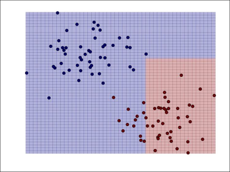
A simple example with two classes is shown in the following figure. The input features in this case have two dimensions, and the feature values are represented on the x and y axes in the figure.
Our task is to train a model that can classify new data points in this two-dimensional space as either one class (red) or the other (blue).
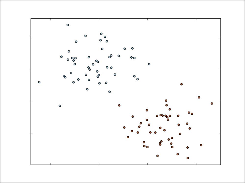
A simple binary classification problem
If we have more than two classes, we would refer to multiclass classification, and classes are typically labeled using integer numbers starting at 0 (for example, five different classes would range from label 0 to 4). An example is shown in the following figure. Again, the input features are assumed to be two-dimensional for ease of illustration.
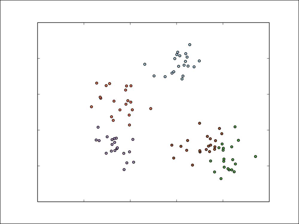
A simple multiclass classification problem
Classification is a form of supervised learning where we train a model with training examples that include known targets or outcomes of interest (that is, the model is supervised with these example outcomes). Classification models can be used in many situations, but a few common examples include:
· Predicting the probability of Internet users clicking on an online advert; here, the classes are binary in nature (that is, click or no click)
· Detecting fraud; again, in this case, the classes are commonly binary (fraud or no fraud)
· Predicting defaults on loans (binary)
· Classifying images, video, or sounds (most often multiclass, with potentially very many different classes)
· Assigning categories or tags to news articles, web pages, or other content (multiclass)
· Discovering e-mail and web spam, network intrusions, and other malicious behavior (binary or multiclass)
· Detecting failure situations, for example in computer systems or networks
· Ranking customers or users in order of probability that they might purchase a product or use a service (this can be framed as classification by predicting probabilities and then ranking in the descending order)
· Predicting customers or users who might stop using a product, service, or provider (called churn)
These are just a few possible use cases. In fact, it is probably safe to say that classification is one of the most widely used machine learning and statistical techniques in modern businesses and especially online businesses.
In this chapter, we will:
· Discuss the types of classification models available in MLlib
· Use Spark to extract the appropriate features from raw input data
· Train a number of classification models using MLlib
· Make predictions with our classification models
· Apply a number of standard evaluation techniques to assess the predictive performance of our models
· Illustrate how to improve model performance using some of the feature-extraction approaches from Chapter 3, Obtaining, Processing, and Preparing Data with Spark
· Explore the impact of parameter tuning on model performance and learn how to use cross-validation to select the most optimal model parameters
Types of classification models
We will explore three common classification models available in Spark: linear models, decision trees, and naïve Bayes models. Linear models, while less complex, are relatively easier to scale to very large datasets. Decision tree is a powerful nonlinear technique that can be a little more difficult to scale up (fortunately, MLlib takes care of this for us!) and more computationally intensive to train, but delivers leading performance in many situations. Naïve Bayes models are more simple but are easy to train efficiently and parallelize (in fact, they require only one pass over the dataset). They can also give reasonable performance in many cases when appropriate feature engineering is used. A naïve Bayes model also provides a good baseline model against which we can measure the performance of other models.
Currently, Spark's MLlib library supports binary classification for linear models, decision trees, and naïve Bayes models and multiclass classification for decision trees and naïve Bayes models. In this book, for simplicity in illustrating the examples, we will focus on the binary case.
Linear models
The core idea of linear models (or generalized linear models) is that we model the predicted outcome of interest (often called the target or dependent variable) as a function of a simple linear predictor applied to the input variables (also referred to as features or independent variables).
y = f(wTx)
Here, y is the target variable, w is the vector of parameters (known as the weight vector), and x is the vector of input features.
wTx is the linear predictor (or vector dot product) of the weight vector w and feature vector x. To this linear predictor, we applied a function f (called the link function).
Linear models can, in fact, be used for both classification and regression, simply by changing the link function. Standard linear regression (covered in the next chapter) uses an identity link (that is, y = wTx directly), while binary classification uses alternative link functions as discussed here.
Let's take a look at the example of online advertising. In this case, the target variable would be 0 (often assigned the class label of -1 in mathematical treatments) if no click was observed for a given advert displayed on a web page (called an impression). The target variable would be 1 if a click occurred. The feature vector for each impression would consist of variables related to the impression event (such as features relating to the user, web page, advert and advertiser, and various other factors relating to the context of the event, such as the type of device used, time of the day, and geolocation).
Thus, we would like to find a model that maps a given input feature vector (advert impression) to a predicted outcome (click or not). To make a prediction for a new data point, we will take the new feature vector (which is unseen, and hence, we do not know what the target variable is) and compute the dot product with our weight vector. We will then apply the relevant link function, and the result is our predicted outcome (after applying a threshold to the prediction, in the case of some models).
Given a set of input data in the form of feature vectors and target variables, we would like to find the weight vector that is the best fit for the data, in the sense that we minimize some error between what our model predicts and the actual outcomes observed. This process is called model fitting, training, or optimization.
More formally, we seek to find the weight vector that minimizes the sum, over all the training examples, of the loss (or error) computed from some loss function. The loss function takes the weight vector, feature vector, and the actual outcome for a given training example as input and outputs the loss. In fact, the loss function itself is effectively specified by the link function; hence, for a given type of classification or regression (that is, a given link function), there is a corresponding loss function.
Tip
For further details on linear models and loss functions, see the linear methods section related to binary classification in the Spark Programming Guide at http://spark.apache.org/docs/latest/mllib-linear-methods.html#binary-classification.Also, see the Wikipedia entry for generalized linear models at http://en.wikipedia.org/wiki/Generalized_linear_model.
While a detailed treatment of linear models and loss functions is beyond the scope of this book, MLlib provides two loss functions suitable to binary classification (you can learn more about them from the Spark documentation). The first one is logistic loss, which equates to a model known as logistic regression, while the second one is the hinge loss, which is equivalent to a linear Support Vector Machine (SVM). Note that the SVM does not strictly fall into the statistical framework of generalized linear models but can be used in the same way as it essentially specifies a loss and link function.
In the following image, we show the logistic loss and hinge loss relative to the actual zero-one loss. The zero-one loss is the true loss for binary classification—it is either zero if the model predicts correctly or one if the model predicts incorrectly. The reason it is not actually used is that it is not a differentiable loss function, so it is not possible to easily compute a gradient and, thus, very difficult to optimize.
The other loss functions are approximations to the zero-one loss that make optimization possible.
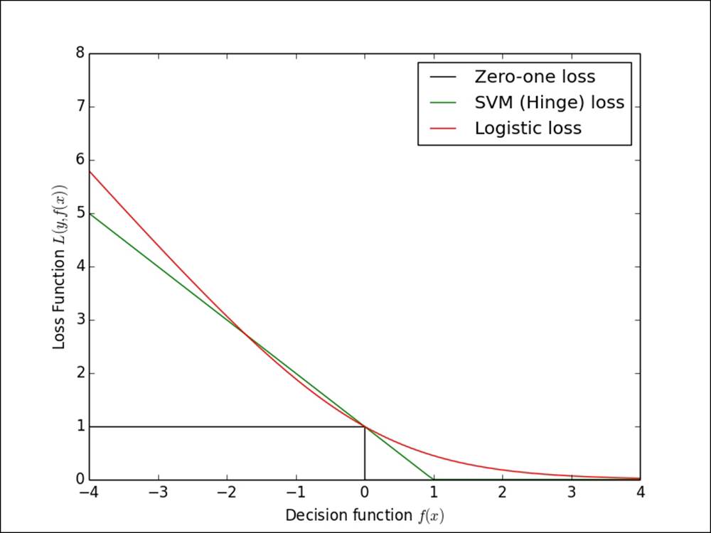
The logistic, hinge and zero-one loss functions
Note
The preceding loss diagram is adapted from the scikit-learn example at http://scikit-learn.org/stable/auto_examples/linear_model/plot_sgd_loss_functions.html.
Logistic regression
Logistic regression is a probabilistic model—that is, its predictions are bounded between 0 and 1, and for binary classification equate to the model's estimate of the probability of the data point belonging to the positive class. Logistic regression is one of the most widely used linear classification models.
As mentioned earlier, the link function used in logistic regression is the logit link:
1 / (1 + exp(-wTx))
The related loss function for logistic regression is the logistic loss:
log(1 + exp(-ywTx))
Here, y is the actual target variable (either 1 for the positive class or -1 for the negative class).
Linear support vector machines
SVM is a powerful and popular technique for regression and classification. Unlike logistic regression, it is not a probabilistic model but predicts classes based on whether the model evaluation is positive or negative.
The SVM link function is the identity link, so the predicted outcome is:
y = wTx
Hence, if the evaluation of wTx is greater than or equal to a threshold of 0, the SVM will assign the data point to class 1; otherwise, the SVM will assign it to class 0 (this threshold is a model parameter of SVM and can be adjusted).
The loss function for SVM is known as the hinge loss and is defined as:
max(0, 1 – ywTx)
SVM is a maximum margin classifier—it tries to find a weight vector such that the classes are separated as much as possible. It has been shown to perform well on many classification tasks, and the linear variant can scale to very large datasets.
Note
SVMs have a large amount of theory behind them, which is beyond the scope of this book, but you can visit http://en.wikipedia.org/wiki/Support_vector_machine and http://www.support-vector-machines.org/ for more details.
In the following image, we have plotted the different decision functions for logistic regression (the blue line) and linear SVM (the red line), based on the simple binary classification example explained earlier.
You can see that the SVM effectively focuses on the points that lie closest to the decision function (the margin lines are shown with red dashes):
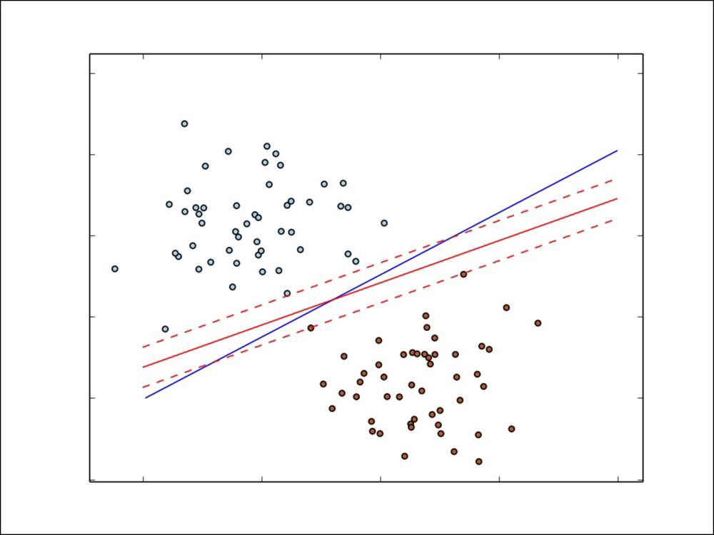
Decision functions for logistic regression and linear SVM for binary classification
The naïve Bayes model
Naïve Bayes is a probabilistic model that makes predictions by computing the probability of a data point that belongs to a given class. A naïve Bayes model assumes that each feature makes an independent contribution to the probability assigned to a class (it assumes conditional independence between features).
Due to this assumption, the probability of each class becomes a function of the product of the probability of a feature occurring, given the class, as well as the probability of this class. This makes training the model tractable and relatively straightforward. The class prior probabilities and feature conditional probabilities are all estimated from the frequencies present in the dataset. Classification is performed by selecting the most probable class, given the features and class probabilities.
An assumption is also made about the feature distributions (the parameters of which are estimated from the data). MLlib implements multinomial naïve Bayes that assumes that the feature distribution is a multinomial distribution that represents non-negative frequency counts of the features.
It is suitable for binary features (for example, 1-of-k encoded categorical features) and is commonly used for text and document classification (where, as we have seen in Chapter 3, Obtaining, Processing, and Preparing Data with Spark, the bag-of-words vector is a typical feature representation).
Note
Take a look at the MLlib - Naive Bayes section in the Spark documentation at http://spark.apache.org/docs/latest/mllib-naive-bayes.html for more information.
The Wikipedia page at http://en.wikipedia.org/wiki/Naive_Bayes_classifier has a more detailed explanation of the mathematical formulation.
Here, we have shown the decision function of naïve Bayes on our simple binary classification example:
Decision function of naïve Bayes for binary classification
Decision trees
Decision tree model is a powerful, nonprobabilistic technique that can capture more complex nonlinear patterns and feature interactions. They have been shown to perform well on many tasks, are relatively easy to understand and interpret, can handle categorical and numerical features, and do not require input data to be scaled or standardized. They are well suited to be included in ensemble methods (for example, ensembles of decision tree models, which are called decision forests).
The decision tree model constructs a tree where the leaves represent a class assignment to class 0 or 1, and the branches are a set of features. In the following figure, we show a simple decision tree where the binary outcome is Stay at home or Go to the beach. The features are the weather outside.
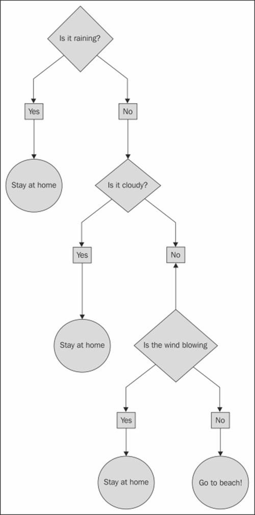
A simple decision tree
The decision tree algorithm is a top-down approach that begins at a root node (or feature), and then selects a feature at each step that gives the best split of the dataset, as measured by the information gain of this split. The information gain is computed from the node impurity (which is the extent to which the labels at the node are similar, or homogenous) minus the weighted sum of the impurities for the two child nodes that would be created by the split. For classification tasks, there are two measures that can be used to select the best split. These are Gini impurity and entropy.
Note
See the MLlib - Decision Tree section in the Spark Programming Guide at http://spark.apache.org/docs/latest/mllib-decision-tree.html for further details on the decision tree algorithm and impurity measures for classification.
In the following screenshot, we have plotted the decision boundary for the decision tree model, as we did for the other models earlier. We can see that the decision tree is able to fit complex, nonlinear models.
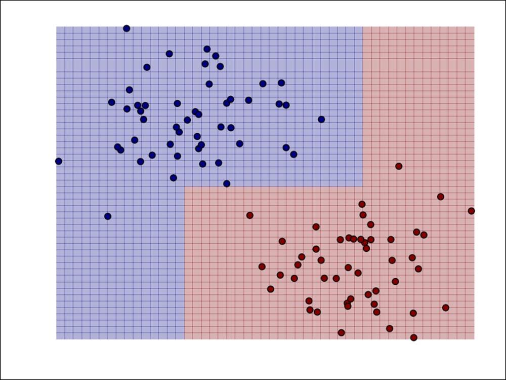
Decision function for a decision tree for binary classification
Extracting the right features from your data
You might recall from Chapter 3, Obtaining, Processing, and Preparing Data with Spark that the majority of machine learning models operate on numerical data in the form of feature vectors. In addition, for supervised learning methods such as classification and regression, we need to provide the target variable (or variables in the case of multiclass situations) together with the feature vector.
Classification models in MLlib operate on instances of LabeledPoint, which is a wrapper around the target variable (called the label) and the feature vector:
case class LabeledPoint(label: Double, features: Vector)
While in most examples of using classification, you will come across existing datasets that are already in the vector format, in practice, you will usually start with raw data that needs to be transformed into features. As we have already seen, this can involve preprocessing and transformation, such as binning numerical features, scaling and normalizing features, and using 1-of-k encodings for categorical features.
Extracting features from the Kaggle/StumbleUpon evergreen classification dataset
In this chapter, we will use a different dataset from the one we used for our recommendation model, as the MovieLens data doesn't have much for us to work with in terms of a classification problem. We will use a dataset from a competition on Kaggle. The dataset was provided by StumbleUpon, and the problem relates to classifying whether a given web page is ephemeral (that is, short lived and will cease being popular soon) or evergreen (that is, persistently popular) on their web content recommendation pages.
Note
The dataset used here can be downloaded from http://www.kaggle.com/c/stumbleupon/data.
Download the training data (train.tsv)—you will need to accept the terms and conditions before downloading the dataset.
You can find more information about the competition at http://www.kaggle.com/c/stumbleupon.
Before we begin, it will be easier for us to work with the data in Spark if we remove the column name header from the first line of the file. Change to the directory in which you downloaded the data (referred to as PATH here) and run the following command to remove the first line and pipe the result to a new file called train_noheader.tsv:
>sed 1d train.tsv > train_noheader.tsv
Now, we are ready to start up our Spark shell (remember to run this command from your Spark installation directory):
>./bin/spark-shell –-driver-memory 4g
You can type in the code that follows for the remainder of this chapter directly into your Spark shell.
In a manner similar to what we did in the earlier chapters, we will load the raw training data into an RDD and inspect it:
val rawData = sc.textFile("/PATH/train_noheader.tsv")
val records = rawData.map(line => line.split("\t"))
records.first()
You will the following on the screen:
Array[String] = Array("http://www.bloomberg.com/news/2010-12-23/ibm-predicts-holographic-calls-air-breathing-batteries-by-2015.html", "4042", ...
You can check the fields that are available by reading through the overview on the dataset page above. The first two columns contain the URL and ID of the page. The next column contains some raw textual content. The next column contains the category assigned to the page. The next 22 columns contain numeric or categorical features of various kinds. The final column contains the target—1 is evergreen, while 0 is non-evergreen.
We'll start off with a simple approach of using only the available numeric features directly. As each categorical variable is binary, we already have a 1-of-k encoding for these variables, so we don't need to do any further feature extraction.
Due to the way the data is formatted, we will have to do a bit of data cleaning during our initial processing by trimming out the extra quotation characters ("). There are also missing values in the dataset; they are denoted by the "?" character. In this case, we will simply assign a zero value to these missing values:
import org.apache.spark.mllib.regression.LabeledPoint
import org.apache.spark.mllib.linalg.Vectors
val data = records.map { r =>
val trimmed = r.map(_.replaceAll("\"", ""))
val label = trimmed(r.size - 1).toInt
val features = trimmed.slice(4, r.size - 1).map(d => if (d == "?") 0.0 else d.toDouble)
LabeledPoint(label, Vectors.dense(features))
}
In the preceding code, we extracted the label variable from the last column and an array of features for columns 5 to 25 after cleaning and dealing with missing values. We converted the label to an Int value and the features to an Array[Double]. Finally, we wrapped the label and features in a LabeledPoint instance, converting the features into an MLlib Vector.
We will also cache the data and count the number of data points:
data.cache
val numData = data.count
You will see that the value of numData is 7395.
We will explore the dataset in more detail a little later, but we will tell you now that there are some negative feature values in the numeric data. As we saw earlier, the naïve Bayes model requires non-negative features and will throw an error if it encounters negative values. So, for now, we will create a version of our input feature vectors for the naïve Bayes model by setting any negative feature values to zero:
val nbData = records.map { r =>
val trimmed = r.map(_.replaceAll("\"", ""))
val label = trimmed(r.size - 1).toInt
val features = trimmed.slice(4, r.size - 1).map(d => if (d == "?") 0.0 else d.toDouble).map(d => if (d < 0) 0.0 else d)
LabeledPoint(label, Vectors.dense(features))
}
Training classification models
Now that we have extracted some basic features from our dataset and created our input RDD, we are ready to train a number of models. To compare the performance and use of different models, we will train a model using logistic regression, SVM, naïve Bayes, and a decision tree. You will notice that training each model looks nearly identical, although each has its own specific model parameters that can be set. MLlib sets sensible defaults in most cases, but in practice, the best parameter setting should be selected using evaluation techniques, which we will cover later in this chapter.
Training a classification model on the Kaggle/StumbleUpon evergreen classification dataset
We can now apply the models from MLlib to our input data. First, we need to import the required classes and set up some minimal input parameters for each model. For logistic regression and SVM, this is the number of iterations, while for the decision tree model, it is the maximum tree depth:
import org.apache.spark.mllib.classification.LogisticRegressionWithSGD
import org.apache.spark.mllib.classification.SVMWithSGD
import org.apache.spark.mllib.classification.NaiveBayes
import org.apache.spark.mllib.tree.DecisionTree
import org.apache.spark.mllib.tree.configuration.Algo
import org.apache.spark.mllib.tree.impurity.Entropy
val numIterations = 10
val maxTreeDepth = 5
Now, train each model in turn. First, we will train logistic regression:
val lrModel = LogisticRegressionWithSGD.train(data, numIterations)
...
14/12/06 13:41:47 INFO DAGScheduler: Job 81 finished: reduce at RDDFunctions.scala:112, took 0.011968 s
14/12/06 13:41:47 INFO GradientDescent: GradientDescent.runMiniBatchSGD finished. Last 10 stochastic losses 0.6931471805599474, 1196521.395699124, Infinity, 1861127.002201189, Infinity, 2639638.049627607, Infinity, Infinity, Infinity, Infinity
lrModel: org.apache.spark.mllib.classification.LogisticRegressionModel = (weights=[-0.11372778986947886,-0.511619752777837,
...
Next up, we will train an SVM model:
val svmModel = SVMWithSGD.train(data, numIterations)
You will see the following output:
...
14/12/06 13:43:08 INFO DAGScheduler: Job 94 finished: reduce at RDDFunctions.scala:112, took 0.007192 s
14/12/06 13:43:08 INFO GradientDescent: GradientDescent.runMiniBatchSGD finished. Last 10 stochastic losses 1.0, 2398226.619666797, 2196192.9647478117, 3057987.2024311484, 271452.9038284356, 3158131.191895948, 1041799.350498323, 1507522.941537049, 1754560.9909073508, 136866.76745605646
svmModel: org.apache.spark.mllib.classification.SVMModel = (weights=[-0.12218838697834929,-0.5275107581589767,
...
Then, we will train the naïve Bayes model; remember to use your special non-negative feature dataset:
val nbModel = NaiveBayes.train(nbData)
The following is the output:
...
14/12/06 13:44:48 INFO DAGScheduler: Job 95 finished: collect at NaiveBayes.scala:120, took 0.441273 s
nbModel: org.apache.spark.mllib.classification.NaiveBayesModel = org.apache.spark.mllib.classification.NaiveBayesModel@666ac612
...
Finally, we will train our decision tree:
val dtModel = DecisionTree.train(data, Algo.Classification, Entropy, maxTreeDepth)
The output is as follows:
...
14/12/06 13:46:03 INFO DAGScheduler: Job 104 finished: collectAsMap at DecisionTree.scala:653, took 0.031338 s
...
total: 0.343024
findSplitsBins: 0.119499
findBestSplits: 0.200352
chooseSplits: 0.199705
dtModel: org.apache.spark.mllib.tree.model.DecisionTreeModel = DecisionTreeModel classifier of depth 5 with 61 nodes
...
Notice that we set the mode, or Algo, of the decision tree to Classification, and we used the Entropy impurity measure.
Using classification models
We now have four models trained on our input labels and features. We will now see how to use these models to make predictions on our dataset. For now, we will use the same training data to illustrate the predict method of each model.
Generating predictions for the Kaggle/StumbleUpon evergreen classification dataset
We will use our logistic regression model as an example (the other models are used in the same way):
val dataPoint = data.first
val prediction = lrModel.predict(dataPoint.features)
The following is the output:
prediction: Double = 1.0
We saw that for the first data point in our training dataset, the model predicted a label of 1 (that is, evergreen). Let's examine the true label for this data point:
val trueLabel = dataPoint.label
You can see the following output:
trueLabel: Double = 0.0
So, in this case, our model got it wrong!
We can also make predictions in bulk by passing in an RDD[Vector] as input:
val predictions = lrModel.predict(data.map(lp => lp.features))
predictions.take(5)
The following is the output:
Array[Double] = Array(1.0, 1.0, 1.0, 1.0, 1.0)
Evaluating the performance of classification models
When we make predictions using our model, as we did earlier, how do we know whether the predictions are good or not? We need to be able to evaluate how well our model performs. Evaluation metrics commonly used in binary classification include prediction accuracy and error, precision and recall, and area under the precision-recall curve, the receiver operating characteristic (ROC) curve, area under ROC curve (AUC), and F-measure.
Accuracy and prediction error
The prediction error for binary classification is possibly the simplest measure available. It is the number of training examples that are misclassified, divided by the total number of examples. Similarly, accuracy is the number of correctly classified examples divided by the total examples.
We can calculate the accuracy of our models in our training data by making predictions on each input feature and comparing them to the true label. We will sum up the number of correctly classified instances and divide this by the total number of data points to get the average classification accuracy:
val lrTotalCorrect = data.map { point =>
if (lrModel.predict(point.features) == point.label) 1 else 0
}.sum
val lrAccuracy = lrTotalCorrect / data.count
The output is as follows:
lrAccuracy: Double = 0.5146720757268425
This gives us 51.5 percent accuracy, which doesn't look particularly impressive! Our model got only half of the training examples correct, which seems to be about as good as a random chance.
Note
Note that the predictions made by the model are not naturally exactly 1 or 0. The output is usually a real number that must be turned into a class prediction. This is done through use of a threshold in the classifier's decision or scoring function.
For example, binary logistic regression is a probabilistic model that returns the estimated probability of class 1 in its scoring function. Thus, a decision threshold of 0.5 is typical. That is, if the estimated probability of being in class 1 is higher than 50 percent, the model decides to classify the point as class 1; otherwise, it will be classified as class 0.
Note that the threshold itself is effectively a model parameter that can be tuned in some models. It also plays a role in evaluation measures, as we will see now.
What about the other models? Let's compute the accuracy for the other three:
val svmTotalCorrect = data.map { point =>
if (svmModel.predict(point.features) == point.label) 1 else 0
}.sum
val nbTotalCorrect = nbData.map { point =>
if (nbModel.predict(point.features) == point.label) 1 else 0
}.sum
Note that the decision tree prediction threshold needs to be specified explicitly, as highlighted here:
val dtTotalCorrect = data.map { point =>
val score = dtModel.predict(point.features)
val predicted = if (score > 0.5) 1 else 0
if (predicted == point.label) 1 else 0
}.sum
We can now inspect the accuracy for the other three models.
First, the SVM model:
val svmAccuracy = svmTotalCorrect / numData
Here is the output for the SVM model:
svmAccuracy: Double = 0.5146720757268425
Next, our naïve Bayes model:
val nbAccuracy = nbTotalCorrect / numData
The output is as follows:
nbAccuracy: Double = 0.5803921568627451
Finally, we compute the accuracy for the decision tree:
val dtAccuracy = dtTotalCorrect / numData
And, the output is:
dtAccuracy: Double = 0.6482758620689655
We can see that both SVM and naïve Bayes also performed quite poorly. The decision tree model is better with 65 percent accuracy, but this is still not particularly high.
Precision and recall
In information retrieval, precision is a commonly used measure of the quality of the results, while recall is a measure of the completeness of the results.
In the binary classification context, precision is defined as the number of true positives (that is, the number of examples correctly predicted as class 1) divided by the sum of true positives and false positives (that is, the number of examples that were incorrectly predicted as class 1). Thus, we can see that a precision of 1.0 (or 100 percent) is achieved if every example predicted by the classifier to be class 1 is, in fact, in class 1 (that is, there are no false positives).
Recall is defined as the number of true positives divided by the sum of true positives and false negatives (that is, the number of examples that were in class 1, but were predicted as class 0 by the model). We can see that a recall of 1.0 (or 100 percent) is achieved if the model doesn't miss any examples that were in class 1 (that is, there are no false negatives).
Generally, precision and recall are inversely related; often, higher precision is related to lower recall and vice versa. To illustrate this, assume that we built a model that always predicted class 1. In this case, the model predictions would have no false negatives because the model always predicts 1; it will not miss any of class 1. Thus, the recall will be 1.0 for this model. On the other hand, the false positive rate could be very high, meaning precision would be low (this depends on the exact distribution of the classes in the dataset).
Precision and recall are not particularly useful as standalone metrics, but are typically used together to form an aggregate or averaged metric. Precision and recall are also dependent on the threshold selected for the model.
Intuitively, below some threshold level, a model will always predict class 1. Hence, it will have a recall of 1, but most likely, it will have low precision. At a high enough threshold, the model will always predict class 0. The model will then have a recall of 0, since itcannot achieve any true positives and will likely have many false negatives. Furthermore, its precision score will be undefined, as it will achieve zero true positives and zero false positives.
The precision-recall (PR) curve shown in the following figure plots precision against recall outcomes for a given model, as the decision threshold of the classifier is changed. The area under this PR curve is referred to as the average precision. Intuitively, an area under the PR curve of 1.0 will equate to a perfect classifier that will achieve 100 percent in both precision and recall.
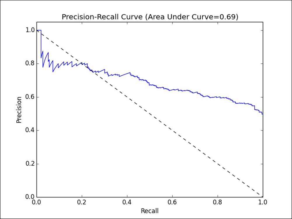
Precision-recall curve
Tip
See http://en.wikipedia.org/wiki/Precision_and_recall and http://en.wikipedia.org/wiki/Average_precision#Average_precision for more details on precision, recall, and area under the PR curve.
ROC curve and AUC
The ROC curve is a concept similar to the PR curve. It is a graphical illustration of the true positive rate against the false positive rate for a classifier.
The true positive rate (TPR) is the number of true positives divided by the sum of true positives and false negatives. In other words, it is the ratio of true positives to all positive examples. This is the same as the recall we saw earlier and is also commonly referred to as sensitivity.
The false positive rate (FPR) is the number of false positives divided by the sum of false positives and true negatives (that is, the number of examples correctly predicted as class 0). In other words, it is the ratio of false positives to all negative examples.
In a manner similar to precision and recall, the ROC curve (plotted in the following figure) represents the classifier's performance tradeoff of TPR against FPR, for different decision thresholds. Each point on the curve represents a different threshold in the decision function for the classifier.
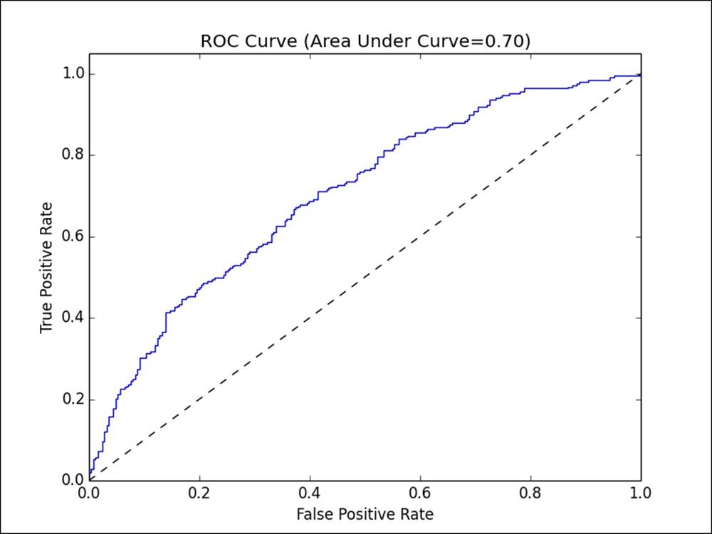
The ROC curve
The area under the ROC curve (commonly referred to as AUC) represents an average value. Again, an AUC of 1.0 will represent a perfect classifier. An area of 0.5 is referred to as the random score. Thus, a model that achieves an AUC of 0.5 is no better than randomly guessing.
Note
As both the area under the PR curve and the area under the ROC curve are effectively normalized (with a minimum of 0 and maximum of 1), we can use these measures to compare models with differing parameter settings and even compare completely different models. Thus, these metrics are popular for model evaluation and selection purposes.
MLlib comes with a set of built-in routines to compute the area under the PR and ROC curves for binary classification. Here, we will compute these metrics for each of our models:
import org.apache.spark.mllib.evaluation.BinaryClassificationMetrics
val metrics = Seq(lrModel, svmModel).map { model =>
val scoreAndLabels = data.map { point =>
(model.predict(point.features), point.label)
}
val metrics = new BinaryClassificationMetrics(scoreAndLabels)
(model.getClass.getSimpleName, metrics.areaUnderPR, metrics.areaUnderROC)
}
As we did previously to train the naïve Bayes model and computing accuracy, we need to use the special nbData version of the dataset that we created to compute the classification metrics:
val nbMetrics = Seq(nbModel).map{ model =>
val scoreAndLabels = nbData.map { point =>
val score = model.predict(point.features)
(if (score > 0.5) 1.0 else 0.0, point.label)
}
val metrics = new BinaryClassificationMetrics(scoreAndLabels)
(model.getClass.getSimpleName, metrics.areaUnderPR, metrics.areaUnderROC)
}
Note that because the DecisionTreeModel model does not implement the ClassificationModel interface that is implemented by the other three models, we need to compute the results separately for this model in the following code:
val dtMetrics = Seq(dtModel).map{ model =>
val scoreAndLabels = data.map { point =>
val score = model.predict(point.features)
(if (score > 0.5) 1.0 else 0.0, point.label)
}
val metrics = new BinaryClassificationMetrics(scoreAndLabels)
(model.getClass.getSimpleName, metrics.areaUnderPR, metrics.areaUnderROC)
}
val allMetrics = metrics ++ nbMetrics ++ dtMetrics
allMetrics.foreach{ case (m, pr, roc) =>
println(f"$m, Area under PR: ${pr * 100.0}%2.4f%%, Area under ROC: ${roc * 100.0}%2.4f%%")
}
Your output will look similar to the one here:
LogisticRegressionModel, Area under PR: 75.6759%, Area under ROC: 50.1418%
SVMModel, Area under PR: 75.6759%, Area under ROC: 50.1418%
NaiveBayesModel, Area under PR: 68.0851%, Area under ROC: 58.3559%
DecisionTreeModel, Area under PR: 74.3081%, Area under ROC: 64.8837%
We can see that all models achieve broadly similar results for the average precision metric.
Logistic regression and SVM achieve results of around 0.5 for AUC. This indicates that they do no better than random chance! Our naïve Bayes and decision tree models fare a little better, achieving an AUC of 0.58 and 0.65, respectively. Still, this is not a very good result in terms of binary classification performance.
Note
While we don't cover multiclass classification here, MLlib provides a similar evaluation class called MulticlassMetrics, which provides averaged versions of many common metrics.
Improving model performance and tuning parameters
So, what went wrong? Why have our sophisticated models achieved nothing better than random chance? Is there a problem with our models?
Recall that we started out by just throwing the data at our model. In fact, we didn't even throw all our data at the model, just the numeric columns that were easy to use. Furthermore, we didn't do a lot of analysis on these numeric features.
Feature standardization
Many models that we employ make inherent assumptions about the distribution or scale of input data. One of the most common forms of assumption is about normally-distributed features. Let's take a deeper look at the distribution of our features.
To do this, we can represent the feature vectors as a distributed matrix in MLlib, using the RowMatrix class. RowMatrix is an RDD made up of vector, where each vector is a row of our matrix.
The RowMatrix class comes with some useful methods to operate on the matrix, one of which is a utility to compute statistics on the columns of the matrix:
import org.apache.spark.mllib.linalg.distributed.RowMatrix
val vectors = data.map(lp => lp.features)
val matrix = new RowMatrix(vectors)
val matrixSummary = matrix.computeColumnSummaryStatistics()
The following code statement will print the mean of the matrix:
println(matrixSummary.mean)
Here is the output:
[0.41225805299526636,2.761823191986623,0.46823047328614004, ...
The following code statement will print the minimum value of the matrix:
println(matrixSummary.min)
Here is the output:
[0.0,0.0,0.0,0.0,0.0,0.0,0.0,-1.0,0.0,0.0,0.0,0.045564223,-1.0, ...
The following code statement will print the maximum value of the matrix:
println(matrixSummary.max)
The output is as follows:
[0.999426,363.0,1.0,1.0,0.980392157,0.980392157,21.0,0.25,0.0,0.444444444, ...
The following code statement will print the variance of the matrix:
println(matrixSummary.variance)
The output of the variance is:
[0.1097424416755897,74.30082476809638,0.04126316989120246, ...
The following code statement will print the nonzero number of the matrix:
println(matrixSummary.numNonzeros)
Here is the output:
[5053.0,7354.0,7172.0,6821.0,6160.0,5128.0,7350.0,1257.0,0.0, ...
The computeColumnSummaryStatistics method computes a number of statistics over each column of features, including the mean and variance, storing each of these in a Vector with one entry per column (that is, one entry per feature in our case).
Looking at the preceding output for mean and variance, we can see quite clearly that the second feature has a much higher mean and variance than some of the other features (you will find a few other features that are similar and a few others that are more extreme). So, our data definitely does not conform to a standard Gaussian distribution in its raw form. To get the data in a more suitable form for our models, we can standardize each feature such that it has zero mean and unit standard deviation. We can do this by subtracting the column mean from each feature value and then scaling it by dividing it by the column standard deviation for the feature:
(x – μ) / sqrt(variance)
Practically, for each feature vector in our input dataset, we can simply perform an element-wise subtraction of the preceding mean vector from the feature vector and then perform an element-wise division of the feature vector by the vector of feature standard deviations. The standard deviation vector itself can be obtained by performing an element-wise square root operation on the variance vector.
As we mentioned in Chapter 3, Obtaining, Processing, and Preparing Data with Spark, we fortunately have access to a convenience method from Spark's StandardScaler to accomplish this.
StandardScaler works in much the same way as the Normalizer feature we used in that chapter. We will instantiate it by passing in two arguments that tell it whether to subtract the mean from the data and whether to apply standard deviation scaling. We will then fitStandardScaler on our input vectors. Finally, we will pass in an input vector to the transform function, which will then return a normalized vector. We will do this within the following map function to preserve the label from our dataset:
import org.apache.spark.mllib.feature.StandardScaler
val scaler = new StandardScaler(withMean = true, withStd = true).fit(vectors)
val scaledData = data.map(lp => LabeledPoint(lp.label, scaler.transform(lp.features)))
Our data should now be standardized. Let's inspect the first row of the original and standardized features:
println(data.first.features)
The output of the preceding line of code is as follows:
[0.789131,2.055555556,0.676470588,0.205882353,
The following code will the first row of the standardized features:
println(scaledData.first.features)
The output is as follows:
[1.1376439023494747,-0.08193556218743517,1.025134766284205,-0.0558631837375738,
As we can see, the first feature has been transformed by applying the standardization formula. We can check this by subtracting the mean (which we computed earlier) from the first feature and dividing the result by the square root of the variance (which we computed earlier):
println((0.789131 - 0.41225805299526636)/ math.sqrt(0.1097424416755897))
The result should be equal to the first element of our scaled vector:
1.137647336497682
We can now retrain our model using the standardized data. We will use only the logistic regression model to illustrate the impact of feature standardization (since the decision tree and naïve Bayes are not impacted by this):
val lrModelScaled = LogisticRegressionWithSGD.train(scaledData, numIterations)
val lrTotalCorrectScaled = scaledData.map { point =>
if (lrModelScaled.predict(point.features) == point.label) 1 else 0
}.sum
val lrAccuracyScaled = lrTotalCorrectScaled / numData
val lrPredictionsVsTrue = scaledData.map { point =>
(lrModelScaled.predict(point.features), point.label)
}
val lrMetricsScaled = new BinaryClassificationMetrics(lrPredictionsVsTrue)
val lrPr = lrMetricsScaled.areaUnderPR
val lrRoc = lrMetricsScaled.areaUnderROC
println(f"${lrModelScaled.getClass.getSimpleName}\nAccuracy: ${lrAccuracyScaled * 100}%2.4f%%\nArea under PR: ${lrPr * 100.0}%2.4f%%\nArea under ROC: ${lrRoc * 100.0}%2.4f%%")
The result should look similar to this:
LogisticRegressionModel
Accuracy: 62.0419%
Area under PR: 72.7254%
Area under ROC: 61.9663%
Simply through standardizing our features, we have improved the logistic regression performance for accuracy and AUC from 50 percent, no better than random, to 62 percent.
Additional features
We have seen that we need to be careful about standardizing and potentially normalizing our features, and the impact on model performance can be serious. In this case, we used only a portion of the features available. For example, we completely ignored the category variable and the textual content in the boilerplate variable column.
This was done for ease of illustration, but let's assess the impact of adding an additional feature such as the category feature.
First, we will inspect the categories and form a mapping of index to category, which you might recognize as the basis for a 1-of-k encoding of this categorical feature:
val categories = records.map(r => r(3)).distinct.collect.zipWithIndex.toMap
val numCategories = categories.size
println(categories)
The output of the different categories is as follows:
Map("weather" -> 0, "sports" -> 6, "unknown" -> 4, "computer_internet" -> 12, "?" -> 11, "culture_politics" -> 3, "religion" -> 8, "recreation" -> 2, "arts_entertainment" -> 9, "health" -> 5, "law_crime" -> 10, "gaming" -> 13, "business" -> 1, "science_technology" -> 7)
The following code will print the number of categories:
println(numCategories)
Here is the output:
14
So, we will need to create a vector of length 14 to represent this feature and assign a value of 1 for the index of the relevant category for each data point. We can then prepend this new feature vector to the vector of other numerical features:
val dataCategories = records.map { r =>
val trimmed = r.map(_.replaceAll("\"", ""))
val label = trimmed(r.size - 1).toInt
val categoryIdx = categories(r(3))
val categoryFeatures = Array.ofDim[Double](numCategories)
categoryFeatures(categoryIdx) = 1.0
val otherFeatures = trimmed.slice(4, r.size - 1).map(d => if (d == "?") 0.0 else d.toDouble)
val features = categoryFeatures ++ otherFeatures
LabeledPoint(label, Vectors.dense(features))
}
println(dataCategories.first)
You should see output similar to what is shown here. You can see that the first part of our feature vector is now a vector of length 14 with one nonzero entry at the relevant category index:
LabeledPoint(0.0, [0.0,1.0,0.0,0.0,0.0,0.0,0.0,0.0,0.0,0.0,0.0,0.0,0.0,0.0,0.789131,2.055555556,0.676470588,0.205882353,0.047058824,0.023529412,0.443783175,0.0,0.0,0.09077381,0.0,0.245831182,0.003883495,1.0,1.0,24.0,0.0,5424.0,170.0,8.0,0.152941176,0.079129575])
Again, since our raw features are not standardized, we should perform this transformation using the same StandardScaler approach that we used earlier before training a new model on this expanded dataset:
val scalerCats = new StandardScaler(withMean = true, withStd = true).fit(dataCategories.map(lp => lp.features))
val scaledDataCats = dataCategories.map(lp => LabeledPoint(lp.label, scalerCats.transform(lp.features)))
We can inspect the features before and after scaling as we did earlier:
println(dataCategories.first.features)
The output is as follows:
0.0,1.0,0.0,0.0,0.0,0.0,0.0,0.0,0.0,0.0,0.0,0.0,0.0,0.0,0.789131,2.055555556 ...
The following code will print the features after scaling:
println(scaledDataCats.first.features)
You will see the following on the screen:
[-0.023261105535492967,2.720728254208072,-0.4464200056407091,-0.2205258360869135, ...
Tip
Note that while the original raw features were sparse (that is, there are many entries that are zero), if we subtract the mean from each entry, we would end up with a non-sparse (dense) representation, as can be seen in the preceding example.
This is not a problem in this case as the data size is small, but often large-scale real-world problems have extremely sparse input data with many features (online advertising and text classification are good examples). In this case, it is not advisable to lose this sparsity, as the memory and processing requirements for the equivalent dense representation can quickly explode with many millions of features. We can use StandardScaler and set withMean to false to avoid this.
We're now ready to train a new logistic regression model with our expanded feature set, and then we will evaluate the performance:
val lrModelScaledCats = LogisticRegressionWithSGD.train(scaledDataCats, numIterations)
val lrTotalCorrectScaledCats = scaledDataCats.map { point =>
if (lrModelScaledCats.predict(point.features) == point.label) 1 else 0
}.sum
val lrAccuracyScaledCats = lrTotalCorrectScaledCats / numData
val lrPredictionsVsTrueCats = scaledDataCats.map { point =>
(lrModelScaledCats.predict(point.features), point.label)
}
val lrMetricsScaledCats = new BinaryClassificationMetrics(lrPredictionsVsTrueCats)
val lrPrCats = lrMetricsScaledCats.areaUnderPR
val lrRocCats = lrMetricsScaledCats.areaUnderROC
println(f"${lrModelScaledCats.getClass.getSimpleName}\nAccuracy: ${lrAccuracyScaledCats * 100}%2.4f%%\nArea under PR: ${lrPrCats * 100.0}%2.4f%%\nArea under ROC: ${lrRocCats * 100.0}%2.4f%%")
You should see output similar to this one:
LogisticRegressionModel
Accuracy: 66.5720%
Area under PR: 75.7964%
Area under ROC: 66.5483%
By applying a feature standardization transformation to our data, we improved both the accuracy and AUC measures from 50 percent to 62 percent, and then, we achieved a further boost to 66 percent by adding the category feature into our model (remember to apply the standardization to our new feature set).
Note
Note that the best model performance in the competition was an AUC of 0.88906 (see http://www.kaggle.com/c/stumbleupon/leaderboard/private).
One approach to achieving performance almost as high is outlined at http://www.kaggle.com/c/stumbleupon/forums/t/5680/beating-the-benchmark-leaderboard-auc-0-878.
Notice that there are still features that we have not yet used; most notably, the text features in the boilerplate variable. The leading competition submissions predominantly use the boilerplate features and features based on the raw textual content to achieve their performance. As we saw earlier, while adding category-improved performance, it appears that most of the variables are not very useful as predictors, while the textual content turned out to be highly predictive.
Going through some of the best performing approaches for these competitions can give you a good idea as to how feature extraction and engineering play a critical role in model performance.
Using the correct form of data
Another critical aspect of model performance is using the correct form of data for each model. Previously, we saw that applying a naïve Bayes model to our numerical features resulted in very poor performance. Is this because the model itself is deficient?
In this case, recall that MLlib implements a multinomial model. This model works on input in the form of non-zero count data. This can include a binary representation of categorical features (such as the 1-of-k encoding covered previously) or frequency data (such as the frequency of occurrences of words in a document). The numerical features we used initially do not conform to this assumed input distribution, so it is probably unsurprising that the model did so poorly.
To illustrate this, we'll use only the category feature, which, when 1-of-k encoded, is of the correct form for the model. We will create a new dataset as follows:
val dataNB = records.map { r =>
val trimmed = r.map(_.replaceAll("\"", ""))
val label = trimmed(r.size - 1).toInt
val categoryIdx = categories(r(3))
val categoryFeatures = Array.ofDim[Double](numCategories)
categoryFeatures(categoryIdx) = 1.0
LabeledPoint(label, Vectors.dense(categoryFeatures))
}
Next, we will train a new naïve Bayes model and evaluate its performance:
val nbModelCats = NaiveBayes.train(dataNB)
val nbTotalCorrectCats = dataNB.map { point =>
if (nbModelCats.predict(point.features) == point.label) 1 else 0
}.sum
val nbAccuracyCats = nbTotalCorrectCats / numData
val nbPredictionsVsTrueCats = dataNB.map { point =>
(nbModelCats.predict(point.features), point.label)
}
val nbMetricsCats = new BinaryClassificationMetrics(nbPredictionsVsTrueCats)
val nbPrCats = nbMetricsCats.areaUnderPR
val nbRocCats = nbMetricsCats.areaUnderROC
println(f"${nbModelCats.getClass.getSimpleName}\nAccuracy: ${nbAccuracyCats * 100}%2.4f%%\nArea under PR: ${nbPrCats * 100.0}%2.4f%%\nArea under ROC: ${nbRocCats * 100.0}%2.4f%%")
You should see the following output:
NaiveBayesModel
Accuracy: 60.9601%
Area under PR: 74.0522%
Area under ROC: 60.5138%
So, by ensuring that we use the correct form of input, we have improved the performance of the naïve Bayes model slightly from 58 percent to 60 percent.
Tuning model parameters
The previous section showed the impact on model performance of feature extraction and selection, as well as the form of input data and a model's assumptions around data distributions. So far, we have discussed model parameters only in passing, but they also play a significant role in model performance.
MLlib's default train methods use default values for the parameters of each model. Let's take a deeper look at them.
Linear models
Both logistic regression and SVM share the same parameters, because they use the same underlying optimization technique of stochastic gradient descent (SGD). They differ only in the loss function applied. If we take a look at the class definition for logistic regression in MLlib, we will see the following definition:
class LogisticRegressionWithSGD private (
private var stepSize: Double,
private var numIterations: Int,
private var regParam: Double,
private var miniBatchFraction: Double)
extends GeneralizedLinearAlgorithm[LogisticRegressionModel] ...
We can see that the arguments that can be passed to the constructor are stepSize, numIterations, regParam, and miniBatchFraction. Of these, all except regParam are related to the underlying optimization technique.
The instantiation code for logistic regression initializes the Gradient, Updater, and Optimizer and sets the relevant arguments for Optimizer (GradientDescent in this case):
private val gradient = new LogisticGradient()
private val updater = new SimpleUpdater()
override val optimizer = new GradientDescent(gradient, updater)
.setStepSize(stepSize)
.setNumIterations(numIterations)
.setRegParam(regParam)
.setMiniBatchFraction(miniBatchFraction)
LogisticGradient sets up the logistic loss function that defines our logistic regression model.
Tip
While a detailed treatment of optimization techniques is beyond the scope of this book, MLlib provides two optimizers for linear models: SGD and L-BFGS. L-BFGS is often more accurate and has fewer parameters to tune.
SGD is the default, while L-BGFS can currently only be used directly for logistic regression via LogisticRegressionWithLBFGS. Try it out yourself and compare the results to those found with SGD.
See http://spark.apache.org/docs/latest/mllib-optimization.html for further details.
To investigate the impact of the remaining parameter settings, we will create a helper function that will train a logistic regression model, given a set of parameter inputs. First, we will import the required classes:
import org.apache.spark.rdd.RDD
import org.apache.spark.mllib.optimization.Updater
import org.apache.spark.mllib.optimization.SimpleUpdater
import org.apache.spark.mllib.optimization.L1Updater
import org.apache.spark.mllib.optimization.SquaredL2Updater
import org.apache.spark.mllib.classification.ClassificationModel
Next, we will define our helper function to train a mode given a set of inputs:
def trainWithParams(input: RDD[LabeledPoint], regParam: Double, numIterations: Int, updater: Updater, stepSize: Double) = {
val lr = new LogisticRegressionWithSGD
lr.optimizer.setNumIterations(numIterations). setUpdater(updater).setRegParam(regParam).setStepSize(stepSize)
lr.run(input)
}
Finally, we will create a second helper function to take the input data and a classification model and generate the relevant AUC metrics:
def createMetrics(label: String, data: RDD[LabeledPoint], model: ClassificationModel) = {
val scoreAndLabels = data.map { point =>
(model.predict(point.features), point.label)
}
val metrics = new BinaryClassificationMetrics(scoreAndLabels)
(label, metrics.areaUnderROC)
}
We will also cache our scaled dataset, including categories, to speed up the multiple model training runs that we will be using to explore these different parameter settings:
scaledDataCats.cache
Iterations
Many machine learning methods are iterative in nature, converging to a solution (the optimal weight vector that minimizes the chosen loss function) over a number of iteration steps. SGD typically requires relatively few iterations to converge to a reasonable solution but can be run for more iterations to improve the solution. We can see this by trying a few different settings for the numIterations parameter and comparing the AUC results:
val iterResults = Seq(1, 5, 10, 50).map { param =>
val model = trainWithParams(scaledDataCats, 0.0, param, new SimpleUpdater, 1.0)
createMetrics(s"$param iterations", scaledDataCats, model)
}
iterResults.foreach { case (param, auc) => println(f"$param, AUC = ${auc * 100}%2.2f%%") }
Your output should look like this:
1 iterations, AUC = 64.97%
5 iterations, AUC = 66.62%
10 iterations, AUC = 66.55%
50 iterations, AUC = 66.81%
So, we can see that the number of iterations has minor impact on the results once a certain number of iterations have been completed.
Step size
In SGD, the step size parameter controls how far in the direction of the steepest gradient the algorithm takes a step when updating the model weight vector after each training example. A larger step size might speed up convergence, but a step size that is too large might cause problems with convergence as good solutions are overshot.
We can see the impact of changing the step size here:
val stepResults = Seq(0.001, 0.01, 0.1, 1.0, 10.0).map { param =>
val model = trainWithParams(scaledDataCats, 0.0, numIterations, new SimpleUpdater, param)
createMetrics(s"$param step size", scaledDataCats, model)
}
stepResults.foreach { case (param, auc) => println(f"$param, AUC = ${auc * 100}%2.2f%%") }
This will give us the following results, which show that increasing the step size too much can begin to negatively impact performance.
0.001 step size, AUC = 64.95%
0.01 step size, AUC = 65.00%
0.1 step size, AUC = 65.52%
1.0 step size, AUC = 66.55%
10.0 step size, AUC = 61.92%
Regularization
We briefly touched on the Updater class in the preceding logistic regression code. An Updater class in MLlib implements regularization. Regularization can help avoid over-fitting of a model to training data by effectively penalizing model complexity. This can be done by adding a term to the loss function that acts to increase the loss as a function of the model weight vector.
Regularization is almost always required in real use cases, but is of particular importance when the feature dimension is very high (that is, the effective number of variable weights that can be learned is high) relative to the number of training examples.
When regularization is absent or low, models can tend to over-fit. Without regularization, most models will over-fit on a training dataset. This is a key reason behind the use of cross-validation techniques for model fitting (which we will cover now).
Conversely, since applying regularization encourages simpler models, model performance can suffer when regularization is high through under-fitting the data.
The forms of regularization available in MLlib are:
· SimpleUpdater: This equates to no regularization and is the default for logistic regression
· SquaredL2Updater: This implements a regularizer based on the squared L2-norm of the weight vector; this is the default for SVM models
· L1Updater: This applies a regularizer based on the L1-norm of the weight vector; this can lead to sparse solutions in the weight vector (as less important weights are pulled towards zero)
Note
Regularization and its relation to optimization is a broad and heavily researched area. Some more information is available from the following links:
· General regularization overview: http://en.wikipedia.org/wiki/Regularization_(mathematics)
· L2 regularization: http://en.wikipedia.org/wiki/Tikhonov_regularization
· Over-fitting and under-fitting: http://en.wikipedia.org/wiki/Overfitting
· Detailed overview of over-fitting and L1 versus L2 regularization: http://citeseerx.ist.psu.edu/viewdoc/download?doi=10.1.1.92.9860&rep=rep1&type=pdf
Let's explore the impact of a range of regularization parameters using SquaredL2Updater:
val regResults = Seq(0.001, 0.01, 0.1, 1.0, 10.0).map { param =>
val model = trainWithParams(scaledDataCats, param, numIterations, new SquaredL2Updater, 1.0)
createMetrics(s"$param L2 regularization parameter", scaledDataCats, model)
}
regResults.foreach { case (param, auc) => println(f"$param, AUC = ${auc * 100}%2.2f%%") }
Your output should look like this:
0.001 L2 regularization parameter, AUC = 66.55%
0.01 L2 regularization parameter, AUC = 66.55%
0.1 L2 regularization parameter, AUC = 66.63%
1.0 L2 regularization parameter, AUC = 66.04%
10.0 L2 regularization parameter, AUC = 35.33%
As we can see, at low levels of regularization, there is not much impact in model performance. However, as we increase regularization, we can see the impact of under-fitting on our model evaluation.
Tip
You will find similar results when using the L1 regularization. Give it a try by performing the same evaluation of regularization parameter against the AUC measure for L1Updater.
Decision trees
The decision tree model we trained earlier was the best performer on the raw data that we first used. We set a parameter called maxDepth, which controls the maximum depth of the tree and, thus, the complexity of the model. Deeper trees result in more complex models that will be able to fit the data better.
For classification problems, we can also select between two measures of impurity: Gini and Entropy.
Tuning tree depth and impurity
We will illustrate the impact of tree depth in a similar manner as we did for our logistic regression model.
First, we will need to create another helper function in the Spark shell:
import org.apache.spark.mllib.tree.impurity.Impurity
import org.apache.spark.mllib.tree.impurity.Entropy
import org.apache.spark.mllib.tree.impurity.Gini
def trainDTWithParams(input: RDD[LabeledPoint], maxDepth: Int, impurity: Impurity) = {
DecisionTree.train(input, Algo.Classification, impurity, maxDepth)
}
Now, we're ready to compute our AUC metric for different settings of tree depth. We will simply use our original dataset in this example since we do not need the data to be standardized.
Tip
Note that decision tree models generally do not require features to be standardized or normalized, nor do they require categorical features to be binary-encoded.
First, train the model using the Entropy impurity measure and varying tree depths:
val dtResultsEntropy = Seq(1, 2, 3, 4, 5, 10, 20).map { param =>
val model = trainDTWithParams(data, param, Entropy)
val scoreAndLabels = data.map { point =>
val score = model.predict(point.features)
(if (score > 0.5) 1.0 else 0.0, point.label)
}
val metrics = new BinaryClassificationMetrics(scoreAndLabels)
(s"$param tree depth", metrics.areaUnderROC)
}
dtResultsEntropy.foreach { case (param, auc) => println(f"$param, AUC = ${auc * 100}%2.2f%%") }
This should output the results shown here:
1 tree depth, AUC = 59.33%
2 tree depth, AUC = 61.68%
3 tree depth, AUC = 62.61%
4 tree depth, AUC = 63.63%
5 tree depth, AUC = 64.88%
10 tree depth, AUC = 76.26%
20 tree depth, AUC = 98.45%
Next, we will perform the same computation using the Gini impurity measure (we omitted the code as it is very similar, but it can be found in the code bundle). Your results should look something like this:
1 tree depth, AUC = 59.33%
2 tree depth, AUC = 61.68%
3 tree depth, AUC = 62.61%
4 tree depth, AUC = 63.63%
5 tree depth, AUC = 64.89%
10 tree depth, AUC = 78.37%
20 tree depth, AUC = 98.87%
As you can see from the preceding results, increasing the tree depth parameter results in a more accurate model (as expected since the model is allowed to get more complex with greater tree depth). It is very likely that at higher tree depths, the model will over-fit the dataset significantly.
There is very little difference in performance between the two impurity measures.
The naïve Bayes model
Finally, let's see the impact of changing the lambda parameter for naïve Bayes. This parameter controls additive smoothing, which handles the case when a class and feature value do not occur together in the dataset.
Tip
See http://en.wikipedia.org/wiki/Additive_smoothing for more details on additive smoothing.
We will take the same approach as we did earlier, first creating a convenience training function and training the model with varying levels of lambda:
def trainNBWithParams(input: RDD[LabeledPoint], lambda: Double) = {
val nb = new NaiveBayes
nb.setLambda(lambda)
nb.run(input)
}
val nbResults = Seq(0.001, 0.01, 0.1, 1.0, 10.0).map { param =>
val model = trainNBWithParams(dataNB, param)
val scoreAndLabels = dataNB.map { point =>
(model.predict(point.features), point.label)
}
val metrics = new BinaryClassificationMetrics(scoreAndLabels)
(s"$param lambda", metrics.areaUnderROC)
}
nbResults.foreach { case (param, auc) => println(f"$param, AUC = ${auc * 100}%2.2f%%")
}
The results of the training are as follows:
0.001 lambda, AUC = 60.51%
0.01 lambda, AUC = 60.51%
0.1 lambda, AUC = 60.51%
1.0 lambda, AUC = 60.51%
10.0 lambda, AUC = 60.51%
We can see that lambda has no impact in this case, since it will not be a problem if the combination of feature and class label not occurring together in the dataset.
Cross-validation
So far in this book, we have only briefly mentioned the idea of cross-validation and out-of-sample testing. Cross-validation is a critical part of real-world machine learning and is central to many model selection and parameter tuning pipelines.
The general idea behind cross-validation is that we want to know how our model will perform on unseen data. Evaluating this on real, live data (for example, in a production system) is risky, because we don't really know whether the trained model is the best in the sense of being able to make accurate predictions on new data. As we saw previously with regard to regularization, our model might have over-fit the training data and be poor at making predictions on data it has not been trained on.
Cross-validation provides a mechanism where we use part of our available dataset to train our model and another part to evaluate the performance of this model. As the model is tested on data that it has not seen during the training phase, its performance, when evaluated on this part of the dataset, gives us an estimate as to how well our model generalizes for the new data points.
Here, we will implement a simple cross-validation evaluation approach using a train-test split. We will divide our dataset into two non-overlapping parts. The first dataset is used to train our model and is called the training set. The second dataset, called the test set or hold-out set, is used to evaluate the performance of our model using our chosen evaluation measure. Common splits used in practice include 50/50, 60/40, and 80/20 splits, but you can use any split as long as the training set is not too small for the model to learn (generally, at least 50 percent is a practical minimum).
In many cases, three sets are created: a training set, an evaluation set (which is used like the above test set to tune the model parameters such as lambda and step size), and a test set (which is never used to train a model or tune any parameters, but is only used to generate an estimated true performance on completely unseen data).
Note
Here, we will explore a simple train-test split approach. There are many cross-validation techniques that are more exhaustive and complex.
One popular example is K-fold cross-validation, where the dataset is split into K non-overlapping folds. The model is trained on K-1 folds of data and tested on the remaining, held-out fold. This is repeated K times, and the results are averaged to give the cross-validation score. The train-test split is effectively like two-fold cross-validation.
Other approaches include leave-one-out cross-validation and random sampling. See the article at http://en.wikipedia.org/wiki/Cross-validation_(statistics) for further details.
First, we will split our dataset into a 60 percent training set and a 40 percent test set (we will use a constant random seed of 123 here to ensure that we get the same results for ease of illustration):
val trainTestSplit = scaledDataCats.randomSplit(Array(0.6, 0.4), 123)
val train = trainTestSplit(0)
val test = trainTestSplit(1)
Next, we will compute the evaluation metric of interest (again, we will use AUC) for a range of regularization parameter settings. Note that here we will use a finer-grained step size between the evaluated regularization parameters to better illustrate the differences in AUC, which are very small in this case:
val regResultsTest = Seq(0.0, 0.001, 0.0025, 0.005, 0.01).map { param =>
val model = trainWithParams(train, param, numIterations, new SquaredL2Updater, 1.0)
createMetrics(s"$param L2 regularization parameter", test, model)
}
regResultsTest.foreach { case (param, auc) => println(f"$param, AUC = ${auc * 100}%2.6f%%")
}
This will compute the results of training on the training set and the results of evaluating on the test set, as shown here:
0.0 L2 regularization parameter, AUC = 66.480874%
0.001 L2 regularization parameter, AUC = 66.480874%
0.0025 L2 regularization parameter, AUC = 66.515027%
0.005 L2 regularization parameter, AUC = 66.515027%
0.01 L2 regularization parameter, AUC = 66.549180%
Now, let's compare this to the results of training and testing on the training set (this is what we were doing previously by training and testing on all data). Again, we will omit the code as it is very similar (but it is available in the code bundle):
0.0 L2 regularization parameter, AUC = 66.260311%
0.001 L2 regularization parameter, AUC = 66.260311%
0.0025 L2 regularization parameter, AUC = 66.260311%
0.005 L2 regularization parameter, AUC = 66.238294%
0.01 L2 regularization parameter, AUC = 66.238294%
So, we can see that when we train and evaluate our model on the same dataset, we generally achieve the highest performance when regularization is lower. This is because our model has seen all the data points, and with low levels of regularization, it can over-fit the data set and achieve higher performance.
In contrast, when we train on one dataset and test on another, we see that generally a slightly higher level of regularization results in better test set performance.
In cross-validation, we would typically find the parameter settings (including regularization as well as the various other parameters such as step size and so on) that result in the best test set performance. We would then use these parameter settings to retrain themodel on all of our data in order to use it to make predictions on new data.
Tip
Recall from Chapter 4, Building a Recommendation Engine with Spark, that we did not cover cross-validation. You can apply the same techniques we used earlier to split the ratings dataset from that chapter into a training and test dataset. You can then try out different parameter settings on the training set while evaluating the MSE and MAP performance metrics on the test set in a manner similar to what we did earlier. Give it a try!
Summary
In this chapter, we covered the various classification models available in Spark MLlib, and we saw how to train models on input data and how to evaluate their performance using standard metrics and measures. We also explored how to apply some of the techniques previously introduced to transform our features. Finally, we investigated the impact of using the correct input data format or distribution on model performance, and we also saw the impact of adding more data to our model, tuning model parameters, and implementing cross-validation.
In the next chapter, we will take a similar approach to delve into MLlib's regression models.
All materials on the site are licensed Creative Commons Attribution-Sharealike 3.0 Unported CC BY-SA 3.0 & GNU Free Documentation License (GFDL)
If you are the copyright holder of any material contained on our site and intend to remove it, please contact our site administrator for approval.
© 2016-2026 All site design rights belong to S.Y.A.