Machine Learning with Spark (2015)
Chapter 6. Building a Regression Model with Spark
In this chapter, we will build on what we covered in Chapter 5, Building a Classification Model with Spark. While classification models deal with outcomes that represent discrete classes, regression models are concerned with target variables that can take any real value. The underlying principle is very similar—we wish to find a model that maps input features to predicted target variables. Like classification, regression is also a form of supervised learning.
Regression models can be used to predict just about any variable of interest. A few examples include the following:
· Predicting stock returns and other economic variables
· Predicting loss amounts for loan defaults (this can be combined with a classification model that predicts the probability of default, while the regression model predicts the amount in the case of a default)
· Recommendations (the Alternating Least Squares factorization model from Chapter 4, Building a Recommendation Engine with Spark, uses linear regression in each iteration)
· Predicting customer lifetime value (CLTV) in a retail, mobile, or other business, based on user behavior and spending patterns
In the following sections, we will:
· Introduce the various types of regression models available in MLlib
· Explore feature extraction and target variable transformation for regression models
· Train a number of regression models using MLlib
· See how to make predictions using the trained models
· Investigate the impact on performance of various parameter settings for regression using cross-validation
Types of regression models
Spark's MLlib library offers two broad classes of regression models: linear models and decision tree regression models.
Linear models are essentially the same as their classification counterparts, the only difference is that linear regression models use a different loss function, related link function, and decision function. MLlib provides a standard least squares regression model (although other types of generalized linear models for regression are planned).
Decision trees can also be used for regression by changing the impurity measure.
Least squares regression
You might recall from Chapter 5, Building a Classification Model with Spark, that there are a variety of loss functions that can be applied to generalized linear models. The loss function used for least squares is the squared loss, which is defined as follows:
½ (wTx - y)2
Here, as for the classification setting, y is the target variable (this time, real valued), w is the weight vector, and x is the feature vector.
The related link function is the identity link, and the decision function is also the identity function, as generally, no thresholding is applied in regression. So, the model's prediction is simply y = wTx.
The standard least squares regression in MLlib does not use regularization. Looking at the squared loss function, we can see that the loss applied to incorrectly predicted points will be magnified since the loss is squared. This means that least squares regression is susceptible to outliers in the dataset and also to over-fitting. Generally, as for classification, we should apply some level of regularization in practice.
Linear regression with L2 regularization is commonly referred to as ridge regression, while applying L1 regularization is called the lasso.
Tip
See the section on linear least squares in the Spark MLlib documentation at http://spark.apache.org/docs/latest/mllib-linear-methods.html#linear-least-squares-lasso-and-ridge-regression for further information.
Decision trees for regression
Just like using linear models for regression tasks involves changing the loss function used, using decision trees for regression involves changing the measure of the node impurity used. The impurity metric is called variance and is defined in the same way as the squared loss for least squares linear regression.
Note
See the MLlib - Decision Tree section in the Spark documentation at http://spark.apache.org/docs/latest/mllib-decision-tree.html for further details on the decision tree algorithm and impurity measure for regression.
Now, we will plot a simple example of a regression problem with only one input variable shown on the x axis and the target variable on the y axis. The linear model prediction function is shown by a red dashed line, while the decision tree prediction function is shown by a green dashed line. We can see that the decision tree allows a more complex, nonlinear model to be fitted to the data.
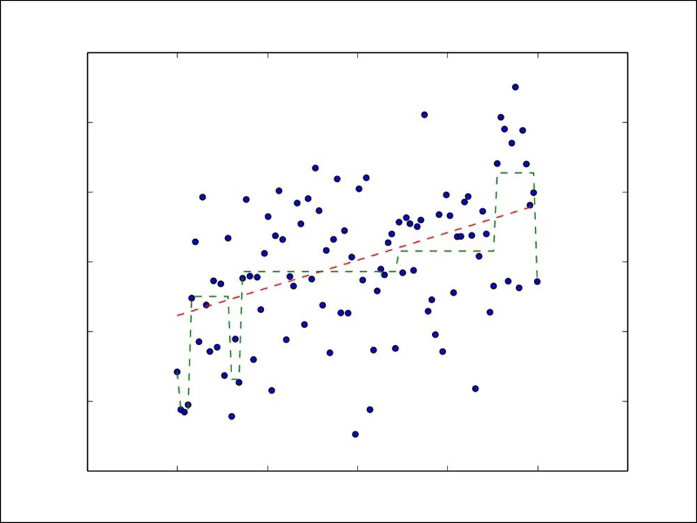
Linear model and decision tree prediction functions for regression
Extracting the right features from your data
As the underlying models for regression are the same as those for the classification case, we can use the same approach to create input features. The only practical difference is that the target is now a real-valued variable, as opposed to a categorical one. TheLabeledPoint class in MLlib already takes this into account, as the label field is of the Double type, so it can handle both cases.
Extracting features from the bike sharing dataset
To illustrate the concepts in this chapter, we will be using the bike sharing dataset. This dataset contains hourly records of the number of bicycle rentals in the capital bike sharing system. It also contains variables related to date and time, weather, and seasonal and holiday information.
Note
The dataset is available at http://archive.ics.uci.edu/ml/datasets/Bike+Sharing+Dataset.
Click on the Data Folder link and then download the Bike-Sharing-Dataset.zip file.
The bike sharing data was enriched with weather and seasonal data by Hadi Fanaee-T at the University of Porto and used in the following paper:
Fanaee-T, Hadi and Gama Joao, Event labeling combining ensemble detectors and background knowledge, Progress in Artificial Intelligence, pp. 1-15, Springer Berlin Heidelberg, 2013.
The paper is available at http://link.springer.com/article/10.1007%2Fs13748-013-0040-3.
Once you have downloaded the Bike-Sharing-Dataset.zip file, unzip it. This will create a directory called Bike-Sharing-Dataset, which contains the day.csv, hour.csv, and the Readme.txt files.
The Readme.txt file contains information on the dataset, including the variable names and descriptions. Take a look at the file, and you will see that we have the following variables available:
· instant: This is the record ID
· dteday: This is the raw date
· season: This is different seasons such as spring, summer, winter, and fall
· yr: This is the year (2011 or 2012)
· mnth: This is the month of the year
· hr: This is the hour of the day
· holiday: This is whether the day was a holiday or not
· weekday: This is the day of the week
· workingday: This is whether the day was a working day or not
· weathersit: This is a categorical variable that describes the weather at a particular time
· temp: This is the normalized temperature
· atemp: This is the normalized apparent temperature
· hum: This is the normalized humidity
· windspeed: This is the normalized wind speed
· cnt: This is the target variable, that is, the count of bike rentals for that hour
We will work with the hourly data contained in hour.csv. If you look at the first line of the dataset, you will see that it contains the column names as a header. You can do this by running the following command:
>head -1 hour.csv
This should output the following result:
instant,dteday,season,yr,mnth,hr,holiday,weekday,workingday,weathersit,temp,atemp,hum,windspeed,casual,registered,cnt
Before we work with the data in Spark, we will again remove the header from the first line of the file using the same sed command that we used previously to create a new file called hour_noheader.csv:
>sed 1d hour.csv > hour_noheader.csv
Since we will be doing some plotting of our dataset later on, we will use the Python shell for this chapter. This also serves to illustrate how to use MLlib's linear model and decision tree functionality from PySpark.
Start up your PySpark shell from your Spark installation directory. If you want to use IPython, which we highly recommend, remember to include the IPYTHON=1 environment variable together with the pylab functionality:
>IPYTHON=1 IPYTHON_OPTS="—pylab" ./bin/pyspark
If you prefer to use IPython Notebook, you can start it with the following command:
>IPYTHON=1 IPYTHON_OPTS=notebook ./bin/pyspark
You can type all the code that follows for the remainder of this chapter directly into your PySpark shell (or into IPython Notebook if you wish to use it).
Tip
Recall that we used the IPython shell in Chapter 3, Obtaining, Processing, and Preparing Data with Spark. Take a look at that chapter and the code bundle for instructions to install IPython.
We'll start as usual by loading the dataset and inspecting it:
path = "/PATH/hour_noheader.csv"
raw_data = sc.textFile(path)
num_data = raw_data.count()
records = raw_data.map(lambda x: x.split(","))
first = records.first()
print first
print num_data
You should see the following output:
[u'1', u'2011-01-01', u'1', u'0', u'1', u'0', u'0', u'6', u'0', u'1', u'0.24', u'0.2879', u'0.81', u'0', u'3', u'13', u'16']
17379
So, we have 17,379 hourly records in our dataset. We have inspected the column names already. We will ignore the record ID and raw date columns. We will also ignore the casual and registered count target variables and focus on the overall count variable, cnt(which is the sum of the other two counts). We are left with 12 variables. The first eight are categorical, while the last 4 are normalized real-valued variables.
To deal with the eight categorical variables, we will use the binary encoding approach with which you should be quite familiar by now. The four real-valued variables will be left as is.
We will first cache our dataset, since we will be reading from it many times:
records.cache()
In order to extract each categorical feature into a binary vector form, we will need to know the feature mapping of each feature value to the index of the nonzero value in our binary vector. Let's define a function that will extract this mapping from our dataset for a given column:
def get_mapping(rdd, idx):
return rdd.map(lambda fields: fields[idx]).distinct().zipWithIndex().collectAsMap()
Our function first maps the field to its unique values and then uses the zipWithIndex transformation to zip the value up with a unique index such that a key-value RDD is formed, where the key is the variable and the value is the index. This index will be the index of the nonzero entry in the binary vector representation of the feature. We will finally collect this RDD back to the driver as a Python dictionary.
We can test our function on the third variable column (index 2):
print "Mapping of first categorical feasture column: %s" % get_mapping(records, 2)
The preceding line of code will give us the following output:
Mapping of first categorical feasture column: {u'1': 0, u'3': 2, u'2': 1, u'4': 3}
Now, we can apply this function to each categorical column (that is, for variable indices 2 to 9):
mappings = [get_mapping(records, i) for i in range(2,10)]
cat_len = sum(map(len, mappings))
num_len = len(records.first()[11:15])
total_len = num_len + cat_len
We now have the mappings for each variable, and we can see how many values in total we need for our binary vector representation:
print "Feature vector length for categorical features: %d" % cat_len
print "Feature vector length for numerical features: %d" % num_len
print "Total feature vector length: %d" % total_len
The output of the preceding code is as follows:
Feature vector length for categorical features: 57
Feature vector length for numerical features: 4
Total feature vector length: 61
Creating feature vectors for the linear model
The next step is to use our extracted mappings to convert the categorical features to binary-encoded features. Again, it will be helpful to create a function that we can apply to each record in our dataset for this purpose. We will also create a function to extract the target variable from each record. We will need to import numpy for linear algebra utilities and MLlib's LabeledPoint class to wrap our feature vectors and target variables:
from pyspark.mllib.regression import LabeledPoint
import numpy as np
def extract_features(record):
cat_vec = np.zeros(cat_len)
i = 0
step = 0
for field in record[2:9]:
m = mappings[i]
idx = m[field]
cat_vec[idx + step] = 1
i = i + 1
step = step + len(m)
num_vec = np.array([float(field) for field in record[10:14]])
return np.concatenate((cat_vec, num_vec))
def extract_label(record):
return float(record[-1])
In the preceding extract_features function, we ran through each column in the row of data. We extracted the binary encoding for each variable in turn from the mappings we created previously. The step variable ensures that the nonzero feature index in the full feature vector is correct (and is somewhat more efficient than, say, creating many smaller binary vectors and concatenating them). The numeric vector is created directly by first converting the data to floating point numbers and wrapping these in a numpy array. The resulting two vectors are then concatenated. The extract_label function simply converts the last column variable (the count) into a float.
With our utility functions defined, we can proceed with extracting feature vectors and labels from our data records:
data = records.map(lambda r: LabeledPoint(extract_label(r), extract_features(r)))
Let's inspect the first record in the extracted feature RDD:
first_point = data.first()
print "Raw data: " + str(first[2:])
print "Label: " + str(first_point.label)
print "Linear Model feature vector:\n" + str(first_point.features)
print "Linear Model feature vector length: " + str(len(first_point.features))
You should see output similar to the following:
Raw data: [u'1', u'0', u'1', u'0', u'0', u'6', u'0', u'1', u'0.24', u'0.2879', u'0.81', u'0', u'3', u'13', u'16']
Label: 16.0
Linear Model feature vector: [1.0,0.0,0.0,0.0,0.0,1.0,0.0,1.0,0.0,0.0,0.0,0.0,0.0,0.0,0.0,0.0,0.0,0.0,0.0,0.0,0.0,0.0,0.0,0.0,0.0,0.0,0.0,0.0,0.0,0.0,0.0,0.0,0.0,0.0,0.0,0.0,1.0,0.0,0.0,0.0,0.0,0.0,0.0,1.0,0.0,0.0,0.0,0.0,0.0,0.0,1.0,0.0,1.0,0.0,0.0,0.0,0.0,0.24,0.2879,0.81,0.0]
Linear Model feature vector length: 61
As we can see, we converted the raw data into a feature vector made up of the binary categorical and real numeric features, and we indeed have a total vector length of 61.
Creating feature vectors for the decision tree
As we have seen, decision tree models typically work on raw features (that is, it is not required to convert categorical features into a binary vector encoding; they can, instead, be used directly). Therefore, we will create a separate function to extract the decision tree feature vector, which simply converts all the values to floats and wraps them in a numpy array:
def extract_features_dt(record):
return np.array(map(float, record[2:14]))
data_dt = records.map(lambda r: LabeledPoint(extract_label(r), extract_features_dt(r)))
first_point_dt = data_dt.first()
print "Decision Tree feature vector: " + str(first_point_dt.features)
print "Decision Tree feature vector length: " + str(len(first_point_dt.features))
The following output shows the extracted feature vector, and we can see that we have a vector length of 12, which matches the number of raw variables we are using:
Decision Tree feature vector: [1.0,0.0,1.0,0.0,0.0,6.0,0.0,1.0,0.24,0.2879,0.81,0.0]
Decision Tree feature vector length: 12
Training and using regression models
Training for regression models using decision trees and linear models follows the same procedure as for classification models. We simply pass the training data contained in a [LabeledPoint] RDD to the relevant train method. Note that in Scala, if we wanted to customize the various model parameters (such as regularization and step size for the SGD optimizer), we are required to instantiate a new model instance and use the optimizer field to access these available parameter setters.
In Python, we are provided with a convenience method that gives us access to all the available model arguments, so we only have to use this one entry point for training. We can see the details of these convenience functions by importing the relevant modules and then calling the help function on the train methods:
from pyspark.mllib.regression import LinearRegressionWithSGD
from pyspark.mllib.tree import DecisionTree
help(LinearRegressionWithSGD.train)
Doing this for the linear model outputs the following documentation:
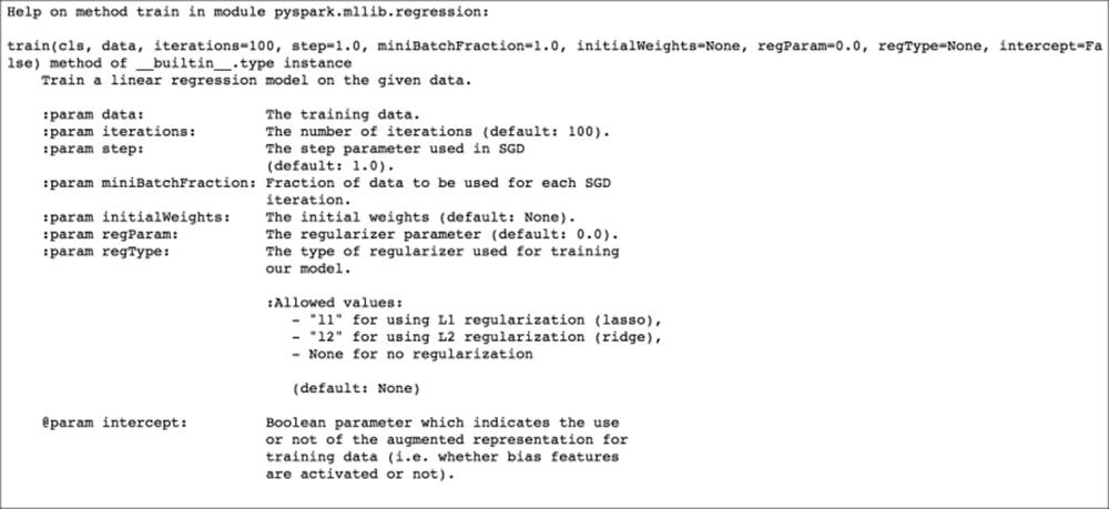
Linear regression help documentation
We can see from the linear regression documentation that we need to pass in the training data at a minimum, but we can set any of the other model parameters using this train method.
Similarly, for the decision tree model, which has a trainRegressor method (in addition to a trainClassifier method for classification models):
help(DecisionTree.trainRegressor)
The preceding code would display the following documentation:
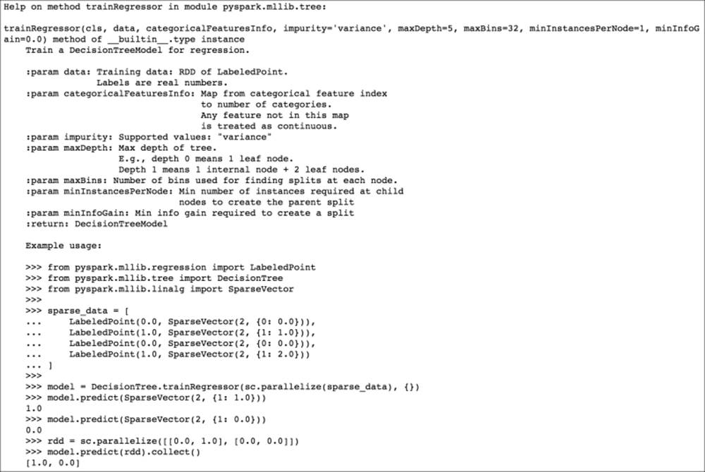
Decision tree regression help documentation
Training a regression model on the bike sharing dataset
We're ready to use the features we have extracted to train our models on the bike sharing data. First, we'll train the linear regression model and take a look at the first few predictions that the model makes on the data:
linear_model = LinearRegressionWithSGD.train(data, iterations=10, step=0.1, intercept=False)
true_vs_predicted = data.map(lambda p: (p.label, linear_model.predict(p.features)))
print "Linear Model predictions: " + str(true_vs_predicted.take(5))
Note that we have not used the default settings for iterations and step here. We've changed the number of iterations so that the model does not take too long to train. As for the step size, you will see why this has been changed from the default a little later. You will see the following output:
Linear Model predictions: [(16.0, 119.30920003093595), (40.0, 116.95463511937379), (32.0, 116.57294610647752), (13.0, 116.43535423855654), (1.0, 116.221247828503)]
Next, we will train the decision tree model simply using the default arguments to the trainRegressor method (which equates to using a tree depth of 5). Note that we need to pass in the other form of the dataset, data_dt, that we created from the raw feature values (as opposed to the binary encoded features that we used for the preceding linear model).
We also need to pass in an argument for categoricalFeaturesInfo. This is a dictionary that maps the categorical feature index to the number of categories for the feature. If a feature is not in this mapping, it will be treated as continuous. For our purposes, we will leave this as is, passing in an empty mapping:
dt_model = DecisionTree.trainRegressor(data_dt,{})
preds = dt_model.predict(data_dt.map(lambda p: p.features))
actual = data.map(lambda p: p.label)
true_vs_predicted_dt = actual.zip(preds)
print "Decision Tree predictions: " + str(true_vs_predicted_dt.take(5))
print "Decision Tree depth: " + str(dt_model.depth())
print "Decision Tree number of nodes: " + str(dt_model.numNodes())
This should output these predictions:
Decision Tree predictions: [(16.0, 54.913223140495866), (40.0, 54.913223140495866), (32.0, 53.171052631578945), (13.0, 14.284023668639053), (1.0, 14.284023668639053)]
Decision Tree depth: 5
Decision Tree number of nodes: 63
Note
This is not as bad as it sounds. While we do not cover it here, the Python code included with this chapter's code bundle includes an example of using categoricalFeaturesInfo. It does not make a large difference to performance in this case.
From a quick glance at these predictions, it appears that the decision tree might do better, as the linear model is quite a way off in its predictions. However, we will apply more stringent evaluation methods to find out.
Evaluating the performance of regression models
We saw in Chapter 5, Building a Classification Model with Spark, that evaluation methods for classification models typically focus on measurements related to predicted class memberships relative to the actual class memberships. These are binary outcomes (either the predicted class is correct or incorrect), and it is less important whether the model just barely predicted correctly or not; what we care most about is the number of correct and incorrect predictions.
When dealing with regression models, it is very unlikely that our model will precisely predict the target variable, because the target variable can take on any real value. However, we would naturally like to understand how far away our predicted values are from the true values, so will we utilize a metric that takes into account the overall deviation.
Some of the standard evaluation metrics used to measure the performance of regression models include the Mean Squared Error (MSE) and Root Mean Squared Error (RMSE), the Mean Absolute Error (MAE), the R-squared coefficient, and many others.
Mean Squared Error and Root Mean Squared Error
MSE is the average of the squared error that is used as the loss function for least squares regression:
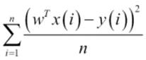
It is the sum, over all the data points, of the square of the difference between the predicted and actual target variables, divided by the number of data points.
RMSE is the square root of MSE. MSE is measured in units that are the square of the target variable, while RMSE is measured in the same units as the target variable. Due to its formulation, MSE, just like the squared loss function that it derives from, effectively penalizes larger errors more severely.
In order to evaluate our predictions based on the mean of an error metric, we will first make predictions for each input feature vector in an RDD of LabeledPoint instances by computing the error for each record using a function that takes the prediction and true target value as inputs. This will return a [Double] RDD that contains the error values. We can then find the average using the mean method of RDDs that contain Double values.
Let's define our squared error function as follows:
def squared_error(actual, pred):
return (pred - actual)**2
Mean Absolute Error
MAE is the average of the absolute differences between the predicted and actual targets:
![]()
MAE is similar in principle to MSE, but it does not punish large deviations as much.
Our function to compute MAE is as follows:
def abs_error(actual, pred):
return np.abs(pred - actual)
Root Mean Squared Log Error
This measurement is not as widely used as MSE and MAE, but it is used as the metric for the Kaggle competition that uses the bike sharing dataset. It is effectively the RMSE of the log-transformed predicted and target values. This measurement is useful when there is a wide range in the target variable, and you do not necessarily want to penalize large errors when the predicted and target values are themselves high. It is also effective when you care about percentage errors rather than the absolute value of errors.
Note
The Kaggle competition evaluation page can be found at https://www.kaggle.com/c/bike-sharing-demand/details/evaluation.
The function to compute RMSLE is shown here:
def squared_log_error(pred, actual):
return (np.log(pred + 1) - np.log(actual + 1))**2
The R-squared coefficient
The R-squared coefficient, also known as the coefficient of determination, is a measure of how well a model fits a dataset. It is commonly used in statistics. It measures the degree of variation in the target variable; this is explained by the variation in the input features. An R-squared coefficient generally takes a value between 0 and 1, where 1 equates to a perfect fit of the model.
Computing performance metrics on the bike sharing dataset
Given the functions we defined earlier, we can now compute the various evaluation metrics on our bike sharing data.
Linear model
Our approach will be to apply the relevant error function to each record in the RDD we computed earlier, which is true_vs_predicted for our linear model:
mse = true_vs_predicted.map(lambda (t, p): squared_error(t, p)).mean()
mae = true_vs_predicted.map(lambda (t, p): abs_error(t, p)).mean()
rmsle = np.sqrt(true_vs_predicted.map(lambda (t, p): squared_log_error(t, p)).mean())
print "Linear Model - Mean Squared Error: %2.4f" % mse
print "Linear Model - Mean Absolute Error: %2.4f" % mae
print "Linear Model - Root Mean Squared Log Error: %2.4f" % rmsle
This outputs the following metrics:
Linear Model - Mean Squared Error: 28166.3824
Linear Model - Mean Absolute Error: 129.4506
Linear Model - Root Mean Squared Log Error: 1.4974
Decision tree
We will use the same approach for the decision tree model, using the true_vs_predicted_dt RDD:
mse_dt = true_vs_predicted_dt.map(lambda (t, p): squared_error(t, p)).mean()
mae_dt = true_vs_predicted_dt.map(lambda (t, p): abs_error(t, p)).mean()
rmsle_dt = np.sqrt(true_vs_predicted_dt.map(lambda (t, p): squared_log_error(t, p)).mean())
print "Decision Tree - Mean Squared Error: %2.4f" % mse_dt
print "Decision Tree - Mean Absolute Error: %2.4f" % mae_dt
print "Decision Tree - Root Mean Squared Log Error: %2.4f" % rmsle_dt
You should see output similar to this:
Decision Tree - Mean Squared Error: 11560.7978
Decision Tree - Mean Absolute Error: 71.0969
Decision Tree - Root Mean Squared Log Error: 0.6259
Looking at the results, we can see that our initial guess about the decision tree model being the better performer is indeed true.
Note
The Kaggle competition leaderboard lists the Mean Value Benchmark score on the test set at about 1.58. So, we see that our linear model performance is not much better. However, the decision tree with default settings achieves a performance of 0.63.
The winning score at the time of writing this book is listed as 0.29504.
Improving model performance and tuning parameters
In Chapter 5, Building a Classification Model with Spark, we showed how feature transformation and selection can make a large difference to the performance of a model. In this chapter, we will focus on another type of transformation that can be applied to a dataset: transforming the target variable itself.
Transforming the target variable
Recall that many machine learning models, including linear models, make assumptions regarding the distribution of the input data as well as target variables. In particular, linear regression assumes a normal distribution.
In many real-world cases, the distributional assumptions of linear regression do not hold. In this case, for example, we know that the number of bike rentals can never be negative. This alone should indicate that the assumption of normality might be problematic. To get a better idea of the target distribution, it is often a good idea to plot a histogram of the target values.
In this section, if you are using IPython Notebook, enter the magic function, %pylab inline, to import pylab (that is, the numpy and matplotlib plotting functions) into the workspace. This will also create any figures and plots inline within the Notebook cell.
If you are using the standard IPython console, you can use %pylab to import the necessary functionality (your plots will appear in a separate window).
We will now create a plot of the target variable distribution in the following piece of code:
targets = records.map(lambda r: float(r[-1])).collect()
hist(targets, bins=40, color='lightblue', normed=True)
fig = matplotlib.pyplot.gcf()
fig.set_size_inches(16, 10)
Looking at the histogram plot, we can see that the distribution is highly skewed and certainly does not follow a normal distribution:
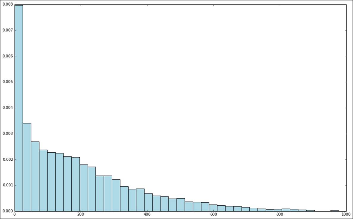
Distribution of raw target variable values
One way in which we might deal with this situation is by applying a transformation to the target variable, such that we take the logarithm of the target value instead of the raw value. This is often referred to as log-transforming the target variable (this transformation can also be applied to feature values).
We will apply a log transformation to the following target variable and plot a histogram of the log-transformed values:
log_targets = records.map(lambda r: np.log(float(r[-1]))).collect()
hist(log_targets, bins=40, color='lightblue', normed=True)
fig = matplotlib.pyplot.gcf()
fig.set_size_inches(16, 10)
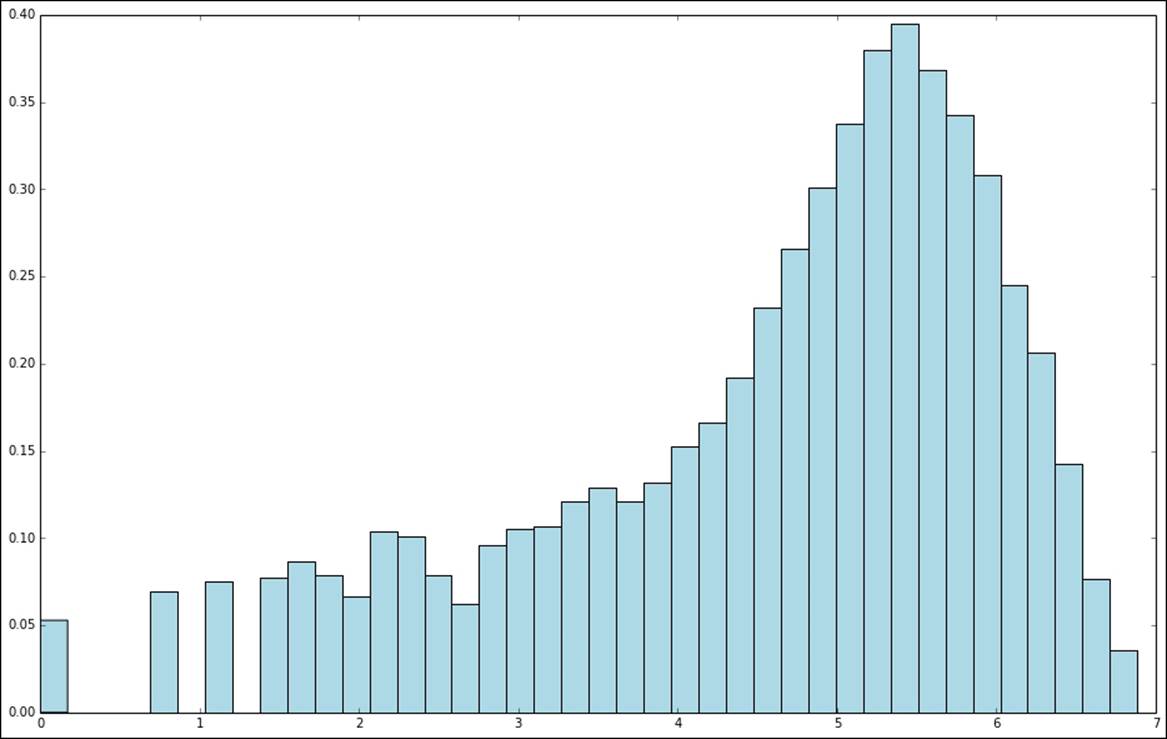
Distribution of log-transformed target variable values
A second type of transformation that is useful in the case of target values that do not take on negative values and, in addition, might take on a very wide range of values, is to take the square root of the variable.
We will apply the square root transform in the following code, once more plotting the resulting target variable distribution:
sqrt_targets = records.map(lambda r: np.sqrt(float(r[-1]))).collect()
hist(sqrt_targets, bins=40, color='lightblue', normed=True)
fig = matplotlib.pyplot.gcf()
fig.set_size_inches(16, 10)
From the plots of the log and square root transformations, we can see that both result in a more even distribution relative to the raw values. While they are still not normally distributed, they are a lot closer to a normal distribution when compared to the original target variable.
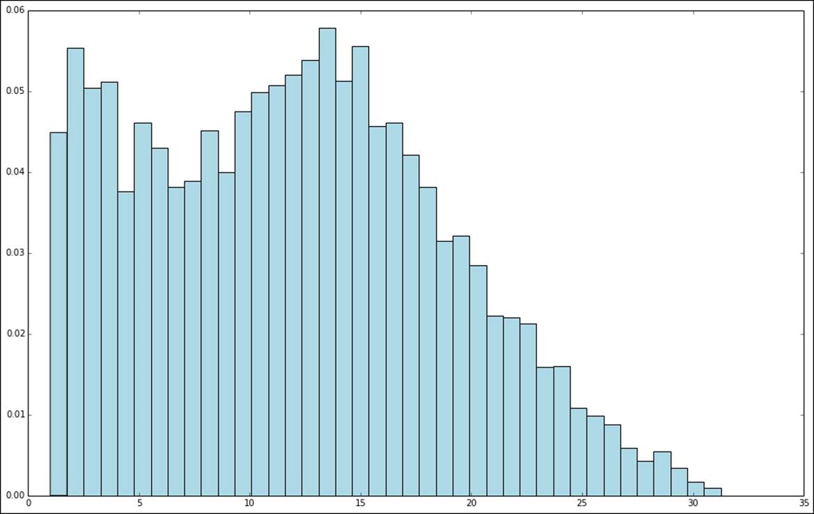
Distribution of square-root-transformed target variable values
Impact of training on log-transformed targets
So, does applying these transformations have any impact on model performance? Let's evaluate the various metrics we used previously on log-transformed data as an example.
We will do this first for the linear model by applying the numpy log function to the label field of each LabeledPoint RDD. Here, we will only transform the target variable, and we will not apply any transformations to the features:
data_log = data.map(lambda lp: LabeledPoint(np.log(lp.label), lp.features))
We will then train a model on this transformed data and form the RDD of predicted versus true values:
model_log = LinearRegressionWithSGD.train(data_log, iterations=10, step=0.1)
Note that now that we have transformed the target variable, the predictions of the model will be on the log scale, as will the target values of the transformed dataset. Therefore, in order to use our model and evaluate its performance, we must first transform the log data back into the original scale by taking the exponent of both the predicted and true values using the numpy exp function. We will show you how to do this in the code here:
true_vs_predicted_log = data_log.map(lambda p: (np.exp(p.label), np.exp(model_log.predict(p.features))))
Finally, we will compute the MSE, MAE, and RMSLE metrics for the model:
mse_log = true_vs_predicted_log.map(lambda (t, p): squared_error(t, p)).mean()
mae_log = true_vs_predicted_log.map(lambda (t, p): abs_error(t, p)).mean()
rmsle_log = np.sqrt(true_vs_predicted_log.map(lambda (t, p): squared_log_error(t, p)).mean())
print "Mean Squared Error: %2.4f" % mse_log
print "Mean Absolue Error: %2.4f" % mae_log
print "Root Mean Squared Log Error: %2.4f" % rmsle_log
print "Non log-transformed predictions:\n" + str(true_vs_predicted.take(3))
print "Log-transformed predictions:\n" + str(true_vs_predicted_log.take(3))
You should see output similar to the following:
Mean Squared Error: 38606.0875
Mean Absolue Error: 135.2726
Root Mean Squared Log Error: 1.3516
Non log-transformed predictions:
[(16.0, 119.30920003093594), (40.0, 116.95463511937378), (32.0, 116.57294610647752)]
Log-transformed predictions:
[(15.999999999999998, 45.860944832110015), (40.0, 43.255903592233274), (32.0, 42.311306147884252)]
If we compare these results to the results on the raw target variable, we see that while we did not improve the MSE or MAE, we improved the RMSLE.
We will perform the same analysis for the decision tree model:
data_dt_log = data_dt.map(lambda lp: LabeledPoint(np.log(lp.label), lp.features))
dt_model_log = DecisionTree.trainRegressor(data_dt_log,{})
preds_log = dt_model_log.predict(data_dt_log.map(lambda p: p.features))
actual_log = data_dt_log.map(lambda p: p.label)
true_vs_predicted_dt_log = actual_log.zip(preds_log).map(lambda (t, p): (np.exp(t), np.exp(p)))
mse_log_dt = true_vs_predicted_dt_log.map(lambda (t, p): squared_error(t, p)).mean()
mae_log_dt = true_vs_predicted_dt_log.map(lambda (t, p): abs_error(t, p)).mean()
rmsle_log_dt = np.sqrt(true_vs_predicted_dt_log.map(lambda (t, p): squared_log_error(t, p)).mean())
print "Mean Squared Error: %2.4f" % mse_log_dt
print "Mean Absolue Error: %2.4f" % mae_log_dt
print "Root Mean Squared Log Error: %2.4f" % rmsle_log_dt
print "Non log-transformed predictions:\n" + str(true_vs_predicted_dt.take(3))
print "Log-transformed predictions:\n" + str(true_vs_predicted_dt_log.take(3))
From the results here, we can see that we actually made our metrics slightly worse for the decision tree:
Mean Squared Error: 14781.5760
Mean Absolue Error: 76.4131
Root Mean Squared Log Error: 0.6406
Non log-transformed predictions:
[(16.0, 54.913223140495866), (40.0, 54.913223140495866), (32.0, 53.171052631578945)]
Log-transformed predictions:
[(15.999999999999998, 37.530779787154508), (40.0, 37.530779787154508), (32.0, 7.2797070993907287)]
Tip
It is probably not surprising that the log transformation results in a better RMSLE performance for the linear model. As we are minimizing the squared error, once we have transformed the target variable to log values, we are effectively minimizing a loss function that is very similar to the RMSLE.
This is good for Kaggle competition purposes, since we can more directly optimize against the competition-scoring metric.
It might or might not be as useful in a real-world situation. This depends on how important larger absolute errors are (recall that RMSLE essentially penalizes relative errors rather than absolute magnitude of errors).
Tuning model parameters
So far in this chapter, we have illustrated the concepts of model training and evaluation for MLlib's regression models by training and testing on the same dataset. We will now use a similar cross-validation approach that we used previously to evaluate the effect on performance of different parameter settings for our models.
Creating training and testing sets to evaluate parameters
The first step is to create a test and training set for cross-validation purposes. Spark's Python API does not yet provide the randomSplit convenience method that is available in Scala. Hence, we will need to create a training and test dataset manually.
One relatively easy way to do this is by first taking a random sample of, say, 20 percent of our data as our test set. We will then define our training set as the elements of the original RDD that are not in the test set RDD.
We can achieve this using the sample method to take a random sample for our test set, followed by using the subtractByKey method, which takes care of returning the elements in one RDD where the keys do not overlap with the other RDD.
Note that subtractByKey, as the name suggests, works on the keys of the RDD elements that consist of key-value pairs. Therefore, here we will use zipWithIndex on our RDD of extracted training examples. This creates an RDD of (LabeledPoint, index) pairs.
We will then reverse the keys and values so that we can operate on the index keys:
data_with_idx = data.zipWithIndex().map(lambda (k, v): (v, k))
test = data_with_idx.sample(False, 0.2, 42)
train = data_with_idx.subtractByKey(test)
Once we have the two RDDs, we will recover just the LabeledPoint instances we need for training and test data, using map to extract the value from the key-value pairs:
train_data = train.map(lambda (idx, p): p)
test_data = test.map(lambda (idx, p) : p)
train_size = train_data.count()
test_size = test_data.count()
print "Training data size: %d" % train_size
print "Test data size: %d" % test_size
print "Total data size: %d " % num_data
print "Train + Test size : %d" % (train_size + test_size)
We can confirm that we now have two distinct datasets that add up to the original dataset in total:
Training data size: 13934
Test data size: 3445
Total data size: 17379
Train + Test size : 17379
The final step is to apply the same approach to the features extracted for the decision tree model:
data_with_idx_dt = data_dt.zipWithIndex().map(lambda (k, v): (v, k))
test_dt = data_with_idx_dt.sample(False, 0.2, 42)
train_dt = data_with_idx_dt.subtractByKey(test_dt)
train_data_dt = train_dt.map(lambda (idx, p): p)
test_data_dt = test_dt.map(lambda (idx, p) : p)
The impact of parameter settings for linear models
Now that we have prepared our training and test sets, we are ready to investigate the impact of different parameter settings on model performance. We will first carry out this evaluation for the linear model. We will create a convenience function to evaluate the relevant performance metric by training the model on the training set and evaluating it on the test set for different parameter settings.
We will use the RMSLE evaluation metric, as it is the one used in the Kaggle competition with this dataset, and this allows us to compare our model results against the competition leaderboard to see how we perform.
The evaluation function is defined here:
def evaluate(train, test, iterations, step, regParam, regType, intercept):
model = LinearRegressionWithSGD.train(train, iterations, step, regParam=regParam, regType=regType, intercept=intercept)
tp = test.map(lambda p: (p.label, model.predict(p.features)))
rmsle = np.sqrt(tp.map(lambda (t, p): squared_log_error(t, p)).mean())
return rmsle
Tip
Note that in the following sections, you might get slightly different results due to some random initialization for SGD. However, your results will be comparable.
Iterations
As we saw when evaluating our classification models, we generally expect that a model trained with SGD will achieve better performance as the number of iterations increases, although the increase in performance will slow down as the number of iterations goes above some minimum number. Note that here, we will set the step size to 0.01 to better illustrate the impact at higher iteration numbers:
params = [1, 5, 10, 20, 50, 100]
metrics = [evaluate(train_data, test_data, param, 0.01, 0.0, 'l2', False) for param in params]
print params
print metrics
The output shows that the error metric indeed decreases as the number of iterations increases. It also does so at a decreasing rate, again as expected. What is interesting is that eventually, the SGD optimization tends to overshoot the optimal solution, and the RMSLE eventually starts to increase slightly:
[1, 5, 10, 20, 50, 100]
[2.3532904530306888, 1.6438528499254723, 1.4869656275309227, 1.4149741941240344, 1.4159641262731959, 1.4539667094611679]
Here, we will use the matplotlib library to plot a graph of the RMSLE metric against the number of iterations. We will use a log scale for the x axis to make the output easier to visualize:
plot(params, metrics)
fig = matplotlib.pyplot.gcf()
pyplot.xscale('log')
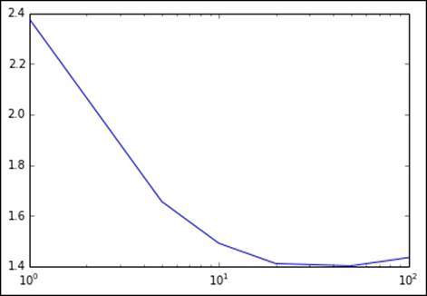
Metrics for varying number of iterations
Step size
We will perform a similar analysis for step size in the following code:
params = [0.01, 0.025, 0.05, 0.1, 1.0]
metrics = [evaluate(train_data, test_data, 10, param, 0.0, 'l2', False) for param in params]
print params
print metrics
The output of the preceding code:
[0.01, 0.025, 0.05, 0.1, 0.5]
[1.4869656275309227, 1.4189071944747715, 1.5027293911925559, 1.5384660954019973, nan]
Now, we can see why we avoided using the default step size when training the linear model originally. The default is set to 1.0, which, in this case, results in a nan output for the RMSLE metric. This typically means that the SGD model has converged to a very poor local minimum in the error function that it is optimizing. This can happen when the step size is relatively large, as it is easier for the optimization algorithm to overshoot good solutions.
We can also see that for low step sizes and a relatively low number of iterations (we used 10 here), the model performance is slightly poorer. However, in the preceding Iterations section, we saw that for the lower step-size setting, a higher number of iterations will generally converge to a better solution.
Generally speaking, setting step size and number of iterations involves a trade-off. A lower step size means that convergence is slower but slightly more assured. However, it requires a higher number of iterations, which is more costly in terms of computation and time, in particular at a very large scale.
Tip
Selecting the best parameter settings can be an intensive process that involves training a model on many combinations of parameter settings and selecting the best outcome. Each instance of model training involves a number of iterations, so this process can be very expensive and time consuming when performed on very large datasets.
The output is plotted here, again using a log scale for the step-size axis:
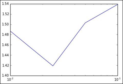
Metrics for varying values of step size
L2 regularization
In Chapter 5, Building a Classification Model with Spark, we saw that regularization has the effect of penalizing model complexity in the form of an additional loss term that is a function of the model weight vector. L2 regularization penalizes the L2-norm of the weight vector, while L1 regularization penalizes the L1-norm.
We expect training set performance to deteriorate with increasing regularization, as the model cannot fit the dataset well. However, we would also expect some amount of regularization that will result in optimal generalization performance as evidenced by the best performance on the test set.
We will evaluate the impact of different levels of L2 regularization in this code:
params = [0.0, 0.01, 0.1, 1.0, 5.0, 10.0, 20.0]
metrics = [evaluate(train_data, test_data, 10, 0.1, param, 'l2', False) for param in params]
print params
print metrics
plot(params, metrics)
fig = matplotlib.pyplot.gcf()
pyplot.xscale('log')
As expected, there is an optimal setting of the regularization parameter with respect to the test set RMSLE:
[0.0, 0.01, 0.1, 1.0, 5.0, 10.0, 20.0]
[1.5384660954019971, 1.5379108106882864, 1.5329809395123755, 1.4900275345312988, 1.4016676336981468, 1.40998359211149, 1.5381771283158705]
This is easiest to see in the following plot (where we once more use the log scale for the regularization parameter axis):
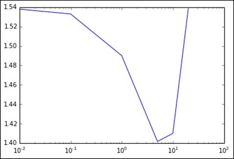
Metrics for varying levels of L2 regularization
L1 regularization
We can apply the same approach for differing levels of L1 regularization:
params = [0.0, 0.01, 0.1, 1.0, 10.0, 100.0, 1000.0]
metrics = [evaluate(train_data, test_data, 10, 0.1, param, 'l1', False) for param in params]
print params
print metrics
plot(params, metrics)
fig = matplotlib.pyplot.gcf()
pyplot.xscale('log')
Again, the results are more clearly seen when plotted in the following graph. We see that there is a much more subtle decline in RMSLE, and it takes a very high value to cause a jump back up. Here, the level of L1 regularization required is much higher than that for the L2 form; however, the overall performance is poorer:
[0.0, 0.01, 0.1, 1.0, 10.0, 100.0, 1000.0]
[1.5384660954019971, 1.5384518080419873, 1.5383237472930684, 1.5372017600929164, 1.5303809928601677, 1.4352494587433793, 4.7551250073268614]
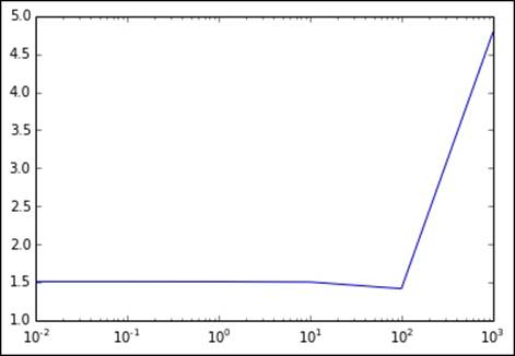
Metrics for varying levels of L1 regularization
Using L1 regularization can encourage sparse weight vectors. Does this hold true in this case? We can find out by examining the number of entries in the weight vector that are zero, with increasing levels of regularization:
model_l1 = LinearRegressionWithSGD.train(train_data, 10, 0.1, regParam=1.0, regType='l1', intercept=False)
model_l1_10 = LinearRegressionWithSGD.train(train_data, 10, 0.1, regParam=10.0, regType='l1', intercept=False)
model_l1_100 = LinearRegressionWithSGD.train(train_data, 10, 0.1, regParam=100.0, regType='l1', intercept=False)
print "L1 (1.0) number of zero weights: " + str(sum(model_l1.weights.array == 0))
print "L1 (10.0) number of zeros weights: " + str(sum(model_l1_10.weights.array == 0))
print "L1 (100.0) number of zeros weights: " + str(sum(model_l1_100.weights.array == 0))
We can see from the results that as we might expect, the number of zero feature weights in the model weight vector increases as greater levels of L1 regularization are applied:
L1 (1.0) number of zero weights: 4
L1 (10.0) number of zeros weights: 20
L1 (100.0) number of zeros weights: 55
Intercept
The final parameter option for the linear model is whether to use an intercept or not. An intercept is a constant term that is added to the weight vector and effectively accounts for the mean value of the target variable. If the data is already centered or normalized, an intercept is not necessary; however, it often does not hurt to use one in any case.
We will evaluate the effect of adding an intercept term to the model here:
params = [False, True]
metrics = [evaluate(train_data, test_data, 10, 0.1, 1.0, 'l2', param) for param in params]
print params
print metrics
bar(params, metrics, color='lightblue')
fig = matplotlib.pyplot.gcf()
We can see from the result and plot that adding the intercept term results in a very slight increase in RMSLE:
[False, True]
[1.4900275345312988, 1.506469812020645]
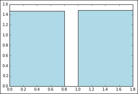
Metrics without and with an intercept
The impact of parameter settings for the decision tree
Decision trees provide two main parameters: maximum tree depth and the maximum number of bins. We will now perform the same evaluation of the effect of parameter settings for the decision tree model. Our starting point is to create an evaluation function for the model, similar to the one used for the linear regression earlier. This function is provided here:
def evaluate_dt(train, test, maxDepth, maxBins):
model = DecisionTree.trainRegressor(train, {}, impurity='variance', maxDepth=maxDepth, maxBins=maxBins)
preds = model.predict(test.map(lambda p: p.features))
actual = test.map(lambda p: p.label)
tp = actual.zip(preds)
rmsle = np.sqrt(tp.map(lambda (t, p): squared_log_error(t, p)).mean())
return rmsle
Tree depth
We would generally expect performance to increase with more complex trees (that is, trees of greater depth). Having a lower tree depth acts as a form of regularization, and it might be the case that as with L2 or L1 regularization in linear models, there is a tree depth that is optimal with respect to the test set performance.
Here, we will try to increase the depths of trees to see what impact they have on test set RMSLE, keeping the number of bins at the default level of 32:
params = [1, 2, 3, 4, 5, 10, 20]
metrics = [evaluate_dt(train_data_dt, test_data_dt, param, 32) for param in params]
print params
print metrics
plot(params, metrics)
fig = matplotlib.pyplot.gcf()
In this case, it appears that the decision tree starts over-fitting at deeper tree levels. An optimal tree depth appears to be around 10 on this dataset.
Note
Notice that our best RMSLE of 0.42 is now quite close to the Kaggle winner of around 0.29!
The output of the tree depth is as follows:
[1, 2, 3, 4, 5, 10, 20]
[1.0280339660196287, 0.92686672078778276, 0.81807794023407532, 0.74060228537329209, 0.63583503599563096, 0.42851360418692447, 0.45500008049779139]
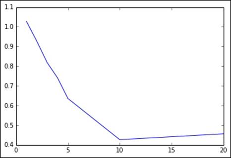
Metrics for different tree depths
Maximum bins
Finally, we will perform our evaluation on the impact of setting the number of bins for the decision tree. As with the tree depth, a larger number of bins should allow the model to become more complex and might help performance with larger feature dimensions. After a certain point, it is unlikely that it will help any more and might, in fact, hinder performance on the test set due to over-fitting:
params = [2, 4, 8, 16, 32, 64, 100]
metrics = [evaluate_dt(train_data_dt, test_data_dt, 5, param) for param in params]
print params
print metrics
plot(params, metrics)
fig = matplotlib.pyplot.gcf()
Here, we will show the output and plot to vary the number of bins (while keeping the tree depth at the default level of 5). In this case, using a small number of bins hurts performance, while there is no impact when we use around 32 bins (the default setting) or more. There seems to be an optimal setting for test set performance at around 16-20 bins:
[2, 4, 8, 16, 32, 64, 100]
[1.3069788763726049, 0.81923394899750324, 0.75745322513058744, 0.62328384445223795, 0.63583503599563096, 0.63583503599563096, 0.63583503599563096]
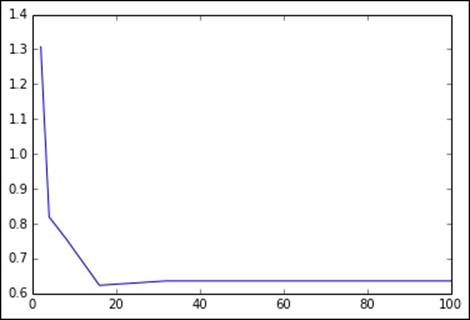
Metrics for different maximum bins
Summary
In this chapter, you saw how to use MLlib's linear model and decision tree functionality in Python within the context of regression models. We explored categorical feature extraction and the impact of applying transformations to the target variable in a regression problem. Finally, we implemented various performance-evaluation metrics and used them to implement a cross-validation exercise that explores the impact of the various parameter settings available in both linear models and decision trees on test set model performance.
In the next chapter, we will cover a different approach to machine learning, that is unsupervised learning, specifically in clustering models.
All materials on the site are licensed Creative Commons Attribution-Sharealike 3.0 Unported CC BY-SA 3.0 & GNU Free Documentation License (GFDL)
If you are the copyright holder of any material contained on our site and intend to remove it, please contact our site administrator for approval.
© 2016-2026 All site design rights belong to S.Y.A.