Biologically Inspired Computer Vision (2015)
Part III
Modelling
Chapter 11
Computational Models of Visual Attention and Applications
Olivier Le Meur and Matei Mancas
11.1 Introduction
Our visual environment contains much more information than we are able to perceive at once. To deal with this large amount of data, human beings have developed biological mechanisms to optimize the visual processing. Visual attention is probably the most important one of these. It allows us to concentrate our biological resources over the most important parts of the visual field.
Visual attention may be differentiated into covert and overt visual attention. Covert attention is defined as paying attention without moving the eyes and could be referred to the act of mentally focusing on a particular area. Overtattention, which involves eye movements, is used both to direct the gaze toward interesting spatial locations and to explore complex visual scenes [1]. As these overt shifts of attention are mainly associated with the execution of saccadic eye movements, this kind of attention is often compared to a window to the mind. Saccade targeting is influenced by top-down factors (the task at hand, behavioral goals, motivational state) and bottom-up factors (both the local and global spatial properties of the visual scene). The bottom-up mechanism, also called stimulus-driven selection, occurs when a target item effortlessly attracts the gaze.
In this chapter, we present models of bottom-up visual attention and their applications. In the first section, we present some models of visual attention. A taxonomy proposed by Borji and Itti [2] is discussed. We will describe more accurately cognitive models, that is, models replicating the behavior of the human visual system (HVS). In the second part, we describe how saliency information can be used. We will see that saliency maps can be used not only in classical image and video applications such as compression but also to envision new applications. In the last section, we will draw someconclusions.
11.2 Models of Visual Attention
Computational saliency models are designed to predict where people look within a visual scene. Most of them are based on the assumption that there exists a unique saliency map in the brain. This saliency map, also called a master map, aims at indicating where the most visually important areas are located. This is a comfortable view for computer scientists as the brain is compared to a computer as illustrated by Figure 11.1. The inputs would come from our different senses, whereas our knowledge would be stored in the memory. The output would be the saliency map, which is used to guide the deployment of attention over the visual space.
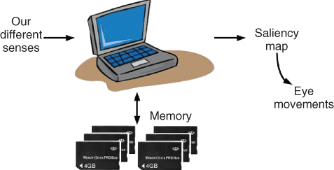
Figure 11.1 The brain as a computer, an unrealistic but convenient hypothesis.
From this assumption which is more than questionable, a number of saliency models have been proposed. In Section 11.2.1, we present a taxonomy and briefly describe the most influential computational models of visual attention.
11.2.1 Taxonomy
Since 1998, the year in which the most influential computational and biologically plausible model of bottom-up visual attention was published by Itti et al. [3], there has been a growing interest in the subject. Indeed, several models, more or less biological and based on different mathematical tools, have been investigated. We proposed in 2009 first saliency taxonomy of models taxonomy [4], which has been significantly improved and extended by Borji and Itti [2].
This taxonomy is composed of eight categories as illustrated by Figure 11.2 (extracted from Ref. [2]). A comprehensive description of these categories is given in Ref. [2]. Here we just give the main features of the four most important categories:
· Cognitive models. Models belonging to this category rely on two seminal works: the feature integration theory (FIT) [5] and a biological plausible architecture [6]. The former relies on the fact that some visual features (commonly called early visual features [7]) are extracted automatically, unconsciously, effortlessly, and very early in the perceptual process. These features such as color, orientation, and shape, to name a few, are automatically separated in parallel throughout the entire visual field. From the FIT, the first biological conceptual architecture has been proposed by Koch and Ullman [6]. This allows the computation of a saliency map based on the assumption that there exists in the brain a single topographic saliency map. Models of this category follow a three-step approach:
· From an input picture, a set of visual features which are known to influence our overt bottom-up visual attention are extracted in a massively parallel manner. These features may be color, orientation, direction of movement, disparity, and so on. Each feature is represented in a topographical map called the feature map.
· A filtering operation is then applied on these maps in order to filter out most of the visually irrelevant information; a particular location of the visual field is considered irrelevant when this location does not differ from its spatial neighborhood.
· Finally, these maps are mixed together to form a saliency map.
In this category, we find the model of Le Meur et al. [8, 9], Marat et al. [10], and so on. We will elaborate further on the Itti and Le Meur models in Section 11.3.
· Information theoretic models. These models are grounded in a probabilistic approach. The assumption is that a rare event is more salient than a non-rare event. The mathematical tool that can simply simulate this behavior is self-information. Self-information is a measure of the amount of information carried out by an event. For a discrete random variable ![]() , defined by
, defined by ![]() and a probability density function, the amount of information of the event
and a probability density function, the amount of information of the event ![]() is given by
is given by ![]() bit/symbol.
bit/symbol.
The first model based on this approach was proposed by Oliva et al. [11]. Bottom-up saliency is given by
11.1 ![]()
where, ![]() denotes a vector of local visual features observed at a given location while
denotes a vector of local visual features observed at a given location while ![]() represents the same visual features but computed over the whole image. When the probability to observe
represents the same visual features but computed over the whole image. When the probability to observe ![]() given
given ![]() is low, the saliency
is low, the saliency ![]() tends to infinity. This approach has been reused and adapted by a number of authors. The main modification is related to the support used to compute the probability density function:
tends to infinity. This approach has been reused and adapted by a number of authors. The main modification is related to the support used to compute the probability density function:
· Oliva et al. [11] determine the probability density function over the whole picture. More recently, Mancas [12] and Riche et al. [13] have computed the saliency map by using a multiscale spatial rarity concept.
· In References [14] and [15], the saliency depends on the local neighborhood from which the probability density function is estimated. The self-information [14] or the mutual information [15] between the probability density functions of the current location and its neighborhood are used to deduce the saliency value.
· A probability density function is learned on a number of natural image patches. Features extracted at a given location are then compared to this prior knowledge in order to infer the saliency value [16].
· Bayesian models. The Bayesian framework is an elegant method to combine current sensory information and prior knowledge concerning the environment (see also Chapter 9). The former is simply the bottom-up saliency which is directly computed from the low-level visual information, whereas the latter is related to the visual inference, also called prior knowledge. This refers to the statistic of visual features in a natural scene, its layout, the scene's category, or its spectral signature. This prior knowledge, which is daily shaped by our visual environment, is one of the most important factors influencing our perception. It acts like visual priming that facilitates perception of the scene and steers our gaze to specific parts.There exist a number of models using prior information, the most well known being the theory of surprise [17], Zhang's model [16], and the model suggested by Torralba et al. [18].
· Spectral analysis models. This kind of model was proposed in 2007 by Hou and Zhang [19]. The saliency is derived from the freqsency domain on the basis of the following assumption: the statistical singularities in the spectrum may be responsible for anomalous regions in the image, where proto-objects are popped up. From this assumption, they defined the spectral residual of an image which is the difference on a log amplitude scale between the amplitude spectrum of the image and its lowpass filtered version. This residual is considered as being the innovation of the image in the frequency domain. The saliency map in the spatial domain is obtained by applying the inverse Fourier transform. The whole process for an image ![]() is given below:
is given below: 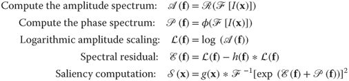
where, ![]() is the radial frequency.
is the radial frequency. ![]() and
and ![]() represent the direct and inverse Fourier transform, respectively.
represent the direct and inverse Fourier transform, respectively. ![]() and
and ![]() are the amplitude and phase spectrum obtained through
are the amplitude and phase spectrum obtained through ![]() and
and ![]() , respectively.
, respectively. ![]() and
and ![]() are two lowpass filters. This first approach has been further extended or modified by taking into account the phase spectrum instead of the amplitude one [20], quaternion representation, and a multiresolution approach [21].
are two lowpass filters. This first approach has been further extended or modified by taking into account the phase spectrum instead of the amplitude one [20], quaternion representation, and a multiresolution approach [21].
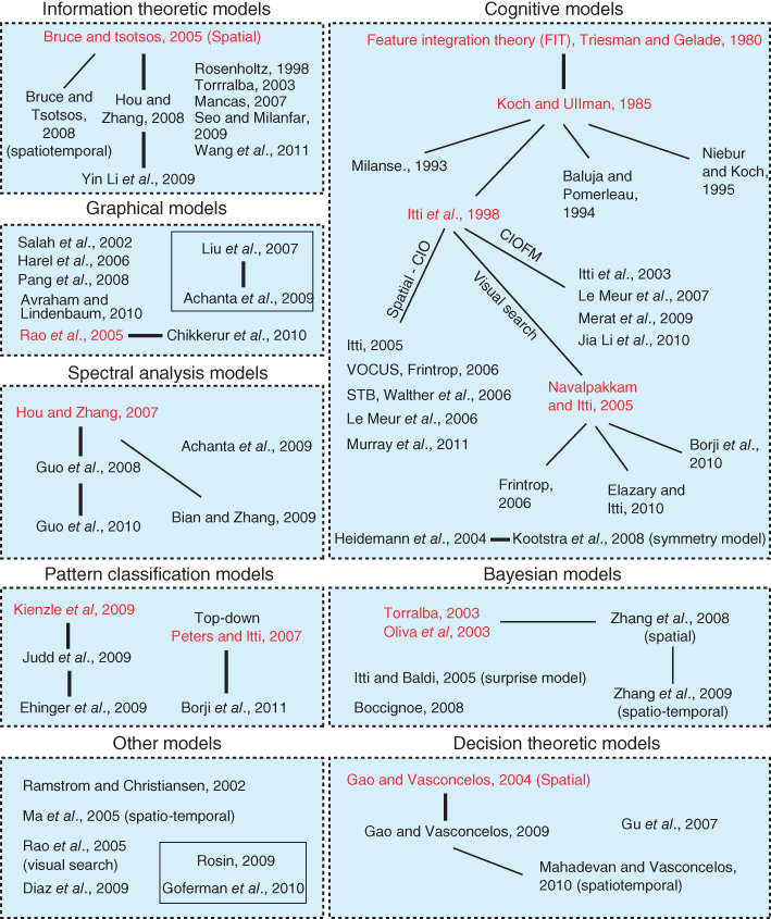
Figure 11.2 Taxonomy of a computational model of visual attention. Courtesy of Borji and Itti [2].
Figure 11.3 illustrates predicted saliency maps computed by different models. The brighter the pixel value is, the higher the saliency.
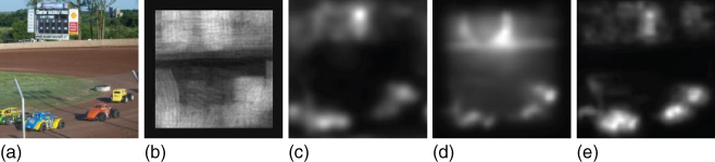
Figure 11.3 (a) Original pictures. (b)–(f) Predicted saliency maps. AIM: attention based on information maximization [14]; AWS: adaptive whitening saliency model [22]; GBVS: graph-based visual saliency [23]; RARE2012: model based on the rarity concept [13].
There exist several methods to evaluate the degree of similarity between the prediction computed by a model and the ground truth. We can classify the metrics into three categories. As a comprehensive review of these metrics is beyond the scope of this chapter, we briefly described these categories below:
· Scanpath-based metrics perform the comparison between two scanpaths. We remind that a scanpath is a series of fixations and saccades.
· Saliency maps-based metrics involve two saliency maps. The most commonly used method is to compare a human saliency map, computed from the eye-tracking data, with a predicted saliency map.
· Hybrid metrics involve the visual fixations and a predicted saliency map. This kind of metric aims at evaluating the saliency located at the spatial locations of visual fixations.
All these methods are described in Ref. [24].
11.3 A Closer Look at Cognitive Models
As briefly presented in the previous section, cognitive saliency models are inspired by the behavior of visual cells and more generally by the properties of the HVS. The modeling strives to reproduce biological mechanisms as faithfully as possible. In the following subsections, we describe two cognitive models: the first is the well-known model proposed by Itti et al. [3]. The second is an extension of Itti's model proposed by Le Meur et al. [8]. We will conclude this section by emphasizing the strengths and limitations of current models.
11.3.1 Itti et al.'s Model [3]
Figure 11.4 shows the architecture of Itti's model. This model could be decomposed into three main steps: topographic feature extraction, within-map saliency competition, and computation of the saliency map, which represents local conspicuity over the entire scene.
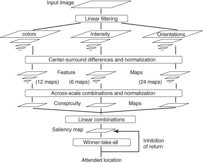
Figure 11.4 Architecture of Itti et al.'s model. The input picture is decomposed into three independent channels (colors, intensity, and orientation) representing early visual features. A Gaussian pyramid is computed on each channel. Center–surround differences and across-scale combinations are applied on the pyramid's scales to infer the saliency map.
The input is first decomposed into three independent channels, namely, colors, intensity, and orientation. A pyramidal representation of these channels is created using Gaussian pyramids with a depth of nine scales.
To determine the local salience of each feature, a center–surround filter is used. The center–surround organization simulates the receptive fields of visual cells. These two regions provide opposite responses. This is implemented as the difference between a fine and a coarse scale for a given feature. This filter is insensitive to uniform illumination and strongly responds on contrast. In total, 42 feature maps (6 for intensity, 12 for color, and 24 for orientation) are obtained.
The final saliency map is then computed by combining the feature maps. Several feature combination strategies were proposed: naive summation, learned linear combination, and contents-based, global, nonlinear amplification and iterative localized interactions. These strategies are defined in Ref. [25].
Figure 11.5 illustrates feature maps and the saliency map computed by Itti's model on a given image. Figure 11.5 (f) and (g) represent the visual scanpaths inferred from the saliency map, following a winner-take-all approach. The first one is composed of the first two fixations, whereas the second is composed of five fixations.
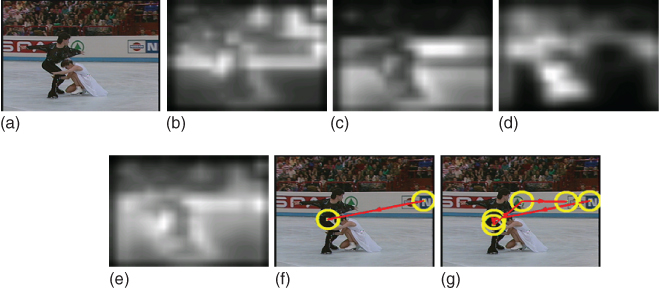
Figure 11.5 Example of feature maps and saliency map computed by Itti's model. (a) Input image; (b)–(d) represent the color, intensity, and orientation feature maps, respectively; (e) saliency map; (f) and (g) represent the visual scanpath with two and five fixations, respectively.
11.3.2 Le Meur et al.'s Model [8]
11.3.2.1 Motivations
In 2006, Le Meur et al. [8] proposed an extension of L. Itti's model. The motivations were twofold:
The first one was simply to improve and deal with the issues of Itti's model [3]. Its most important drawback relates to the combination and normalization of the feature maps which come from different visual modalities. In other words, the question is how to combine color, luminance, and orientation information to get a saliency value. A simple and efficient method is to normalize all feature maps in the same dynamic range (e.g., between 0 and 255) and to sum them into the saliency map. Although efficient, this approach does not take into account the relative importance and the intrinsic features of one dimension compared to another.
The second motivation was the willingness to incorporate into the model important properties of the HVS. For instance, we do not perceive all information present in the visual field with the same accuracy. Contrast sensitivity functions (CSFs) and visual masking are then at the heart of Le Meur's model.
11.3.2.2 Global Architecture
Figure 11.6 illustrates the global architecture of Le Meur et al.'s model. The input picture is first transformed into an opponent-color space from which three components ![]() , representing the achromatic, the reddish-greenish, and the bluish-yellowish signals respectively are obtained. Figure 11.7 gives an example of these three components.
, representing the achromatic, the reddish-greenish, and the bluish-yellowish signals respectively are obtained. Figure 11.7 gives an example of these three components.
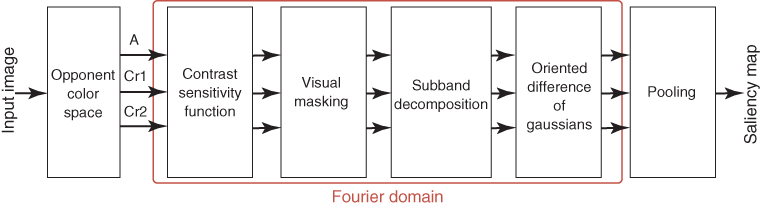
Figure 11.6 Architecture of Le Meur et al.'s model. The input picture is decomposed into one achromatic (A) and two chromatic components (![]() and
and ![]() ). The Fourier transform is then used to encode all of the spatial frequencies present in these three components. Several filters are eventually applied on the magnitude spectrum to get the saliency map.
). The Fourier transform is then used to encode all of the spatial frequencies present in these three components. Several filters are eventually applied on the magnitude spectrum to get the saliency map.

Figure 11.7 Projection of the input color image into an opponent-color space. (a) Input image; (b) achromatic component; (c) ![]() channel (reddish-greenish); (d)
channel (reddish-greenish); (d) ![]() channel (bluish-yellowish).
channel (bluish-yellowish).
CSFs and visual masking are then applied in the frequency domain on the three components of the color space. The former normalizes the dynamic range of ![]() in terms of visibility threshold. In this model, the CSF proposed by Daly [26] is used to normalize the Fourier spectrum of the achromatic component. This CSF model is a function of many parameters, including radial spatial frequency, orientation, luminance levels, image size, image eccentricity, and viewing distance. This model behaves as an anisotropic bandpass filter, with greater sensitivity to horizontal and vertical spatial frequencies than to diagonal frequencies. Figure 11.8(a) shows the transfer function of the anisotropic 2D CSF used to normalize the achromatic component. Regarding the color components, the anisotropic CSFs defined in Ref. [27] are used. They are defined as follows:
in terms of visibility threshold. In this model, the CSF proposed by Daly [26] is used to normalize the Fourier spectrum of the achromatic component. This CSF model is a function of many parameters, including radial spatial frequency, orientation, luminance levels, image size, image eccentricity, and viewing distance. This model behaves as an anisotropic bandpass filter, with greater sensitivity to horizontal and vertical spatial frequencies than to diagonal frequencies. Figure 11.8(a) shows the transfer function of the anisotropic 2D CSF used to normalize the achromatic component. Regarding the color components, the anisotropic CSFs defined in Ref. [27] are used. They are defined as follows:
11.2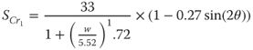
11.3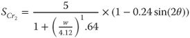
where, ![]() is the radial pulsation (expressed in degrees of visual angle) and
is the radial pulsation (expressed in degrees of visual angle) and ![]() the orientation (expressed in degrees).
the orientation (expressed in degrees).
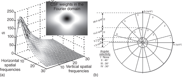
Figure 11.8 Normalization and perceptual subband decomposition in the Fourier domain: (a) anisotropic CSF proposed by Ref. [26]. This CSF is applied on the achromatic component. The inset represents the CSF weights in the Fourier domain (the center of the image represents the lowest radial frequencies, whereas the four corners indicate the highest radial frequencies). (b) The amplitude spectrum of the achromatic component is decomposed into 17 subbands [27].
Once all visual features are expressed in terms of the visibility threshold, visual masking is applied in order to take into account the influence of the spatial context. This aims to increase or to decrease the visibility threshold. For instance, the visibility threshold of a given area tends to increase when its local neighborhood is spatially complex. All details can be found in Refs [8, 27].
The 2D spatial frequency domain is then decomposed into a number of subbands which may be regarded as the neural image corresponding to a population of visual cells tuned to both a range of spatial frequencies and orientations. These decompositions, which have been defined thanks to psychophysics experiments, leads to 17 subbands for the achromatic component and 5 subbands for chromatic components. Figure 11.8 (b) gives the radial frequencies and the angular selectivity of the 17 subbands obtained from the achromatic component decomposition. The decomposition is organized into four crowns, namely I, II, III, and IV:
· Crown I represents the lowest frequencies of the achromatic component;
· Crown II is decomposed into four subbands with an angular selectivity equal to 45![]() ;
;
· Crowns III and IV are decomposed into six subbands with an angular selectivity equal to 30![]() .
.
Figure 11.9 presents the achromatic subbands of crowns I and II for the input picture illustrated in Figure 11.7 (b).
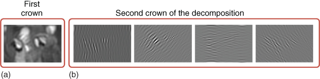
Figure 11.9 Achromatic subbands of the achromatic component of image illustrated on Figure 11.7. Only the subbands corresponding to the first crown (a) and the second crown (b) are shown.
An oriented center–surround filter is then used to filter out redundant information and this behaves as within-map competition to infer the local conspicuity. This filter is implemented in the model as a difference of Gaussians, also called a Mexican hat. The difference of Gaussians is indeed a classical method for simulating the behavior of visual cells.
The filtered subbands are then combined into a unique saliency map. There exist a number of pooling strategies described in Ref. [28]. The simplest one consists in normalizing and summing all subbands into the final saliency map. This method is called NS, standing for normalization and sum.
Figure 11.10 illustrates saliency maps computed by the proposed method (the fusion called NS is used here). Saliency models perform well for this kind of images for which there is a salient object on a simple background. The model performance significantly decreases in the presence of high-level information [29] such as faces (whether they are human or animal, real or cartoon, frontal or sideways, masked or not, in-focus or blurred), text (whether it is font, size, or quality), and horizon line, which strongly attracts our attention [30]. The model performance is also low when the dispersion between observers is high.
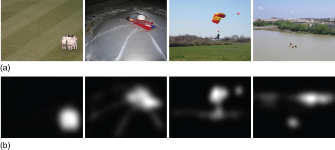
Figure 11.10 Examples of saliency maps predicted by the proposed model. (a) Original images. (b) Predicted saliency maps.
11.3.3 Limitations
Although computational models of visual attention have substantial power to predict where we look within a scene, improvement is still required. As mentioned previously, computational models of visual attention perform quite well for simple images in which one region stands out from the background. However, when the scene contains high-level information, such as face, text, or horizon line, it becomes much more difficult to accurately predict the salient areas. Some models already embed specific detectors such as face [31], text [31], or horizon line [31, 32]. These detectors allow to improve undeniably the performance of models to predict salient areas. As well discussed in Ref. [29], knowledge of and the ability to define the high-level visual features required to improve models is one of the major challenges faced by researchers studying visual attention.
As mentioned in Section 11.2, there exist a number of models which are more or less biologically plausible. They all output a 2D static saliency map. Although this representation is a convenient way to indicate where we look within a scene, some important aspects of our visual system are clearly overlooked. When viewing a scene, our eyes alternate between fixations and saccades, jumping from one specific location to another. This visual exploration within a visual scene is a highly dynamic process in which time plays an important role. However, most computational implementations of human visual attention could be boiled down to a simple nondynamic map of interest. The next generation of visual attention models should be able to consider, at least, the temporal dimension in order to account for the complexity of our visual system.
11.4 Applications
The applications of saliency maps are numerous. In this section, a non-exhaustive list of saliency-based applications is first given. After a brief description of these applications, we will emphasize two of them: prediction of the picture's memorability and quality estimation.
11.4.1 Saliency-Based Applications: A Brief Review
We present in the following a list of saliency-based applications.
· Computer graphics. In this field, saliency can serve several goals including rendering and performing artistic effects. Concerning the former,the idea is to render salient areas with higher accuracy than non-salient parts [33, 34]. The latter consists in modifying an image by removing details while preserving salient areas. DeCarlo and Santella [35] used saliency maps for this purpose.
· Compression. Predicting where people look within a scene can be used to locally adapt the visual compression. The simplest way is to allocate more bit budget to salient parts compared to non-salient areas [36]. This saliency-based bit budget allocation could potentially improve on the overall level of observer satisfaction. This reallocation is more efficient when the target bit budget is rather low. At medium to high bit rate, the saliency-based allocation is more questionable.
· Extraction of object of interest. This application consists in extracting in an automatic manner the most interesting object in an image or video sequence. From an input image, an object with well-defined boundaries is detected based on its saliency. A renewed interest in this subject can be observed since 2010 [37, 38]. A number of datasets serving as ground truth have been recently released and can be used to benchmark methods.
· Images optimization for communication, advertisement and marketing. These are websites, ads, or other documents need to make the important information visible enough to be seen in a very short time. Attention models can help to find the best configuration of a website for example. Some approaches use saliency to optimize the location of an item in a gallery and others to optimize the location (and time in case of videos) where/when to introduce ads in a document.
Besides these applications, we would like to mention robotics, recognition and retrieval, video summarization, and medical and security applications, for the sake of completeness.
11.4.2 Predicting Memorability of Pictures
The study of image memorability in computer science is a recent topic [39–41]. From the first attempts, it appears that it is possible to predict the degree of an image's memorability quite well. In this section, we present the concept of memorability of pictures, the relationship between memorability and eye movement, and finally the computational models predicting the extent to which a picture is memorable.
11.4.2.1 Memorability Definition
Humans have an amazing visual memory. Only a few seconds is enough to memorize an image [42]. However, not all images are equally memorable. Some are very easy to memorize and to recall, whereas the memorization task appears to be much more difficult for other pictures. Isola et al. [39] were the first to build a large dataset of pictures associated with their own memorability score. The score varies between 0 and 1: ![]() indicates that the picture is not memorable at all while
indicates that the picture is not memorable at all while ![]() indicates the highest score of memorability. Memorability has been quantified by performing a visual memory game. Six hundred and sixty five participants were involved in a test to score the memorability of 2222 images. This dataset is freely available on the author's website.
indicates the highest score of memorability. Memorability has been quantified by performing a visual memory game. Six hundred and sixty five participants were involved in a test to score the memorability of 2222 images. This dataset is freely available on the author's website.
From this large amount of data, Isola et al. [39] investigated the contributions of different factors and envisioned the first computational model for predicting memorability scores.
11.4.2.2 Memorability and Eye Movement
Mancas and Le Meur [41] performed an eye-tracking experiment in order to investigate whether the memorability of a picture has an influence on visual deployment. For this, ![]() pictures were extracted from the dataset proposed by Isola et al. [39]. They are organized into three classes of statistically different memorability, each composed of
pictures were extracted from the dataset proposed by Isola et al. [39]. They are organized into three classes of statistically different memorability, each composed of ![]() pictures. The first class consists of the most memorable pictures (
pictures. The first class consists of the most memorable pictures (![]() , score
, score ![]() ), the second of typical memorability (
), the second of typical memorability (![]() , score
, score ![]() ), and the third of the least memorable images (
), and the third of the least memorable images (![]() , score
, score ![]() ).
).
As visual attention might be a step toward memory, image memorability should influence the intrinsic parameters of eye movements such as the duration of visual fixations, the congruency between observers, and the saccade lengths. From the collected eye-tracking data, the visual behavior of participants is analyzed according to the picture's memorability. Figure 11.11 illustrates this point. Four pictures are depicted; the first two pictures have a low memorability score whereas this score is high for the last two pictures. The first picture has a memorability score of ![]() , whereas the last one has a memorability score of
, whereas the last one has a memorability score of ![]() . The average fixation durations for these two pictures are 391 and 278 ms, respectively. The average lengths of saccades are 2.39 and 2.99 degree of visual angle, respectively.
. The average fixation durations for these two pictures are 391 and 278 ms, respectively. The average lengths of saccades are 2.39 and 2.99 degree of visual angle, respectively.
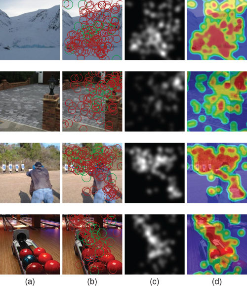
Figure 11.11 (a) Original pictures; (b) fixation map (a green circle represents the first fixation of observers); (c) saliency map; and (d) heat map. From top to bottom, the memorability score is ![]() ,
, ![]() ,
, ![]() , and
, and ![]() , respectively (from a low to high memorability).
, respectively (from a low to high memorability).
From the proposed experiment in Ref. [41], several conclusions have been drawn. First, the fixation durations increase with the degree of memorability of the pictures. This trend is especially noticeable just after the stimuli onset. Fixations are the longest when observers watch memorable pictures. A statistically significant difference is found between fixation durations when the top 20 most memorable and the bottom 20 least memorable pictures are considered. This difference is confirmedfor different viewing times.
The congruency between observers watching the same stimulus is the second indicator that has been analyzed. It indicates the degree of similarity between observers' fixations. A high congruency would mean that observers look at the same regions of the stimuli. Otherwise, the congruency is low. Generally, the consistency between visual fixations of different participants is high just after the stimulus onset but progressively decreases over time [43]. To quantify inter-observer congruency, two metrics can be used: receiver operating characteristic (ROC) [24] or a bounding box approach [44]. The former is a parametric approach contrary to the latter. The main drawback of the bounding box approach is its high sensitivity to outliers. A value of 1 indicates a perfect similarity between observers, whereas the value ![]() corresponds to the minimal congruency. Results of Ref. [41] indicate that the congruency is highest on the class
corresponds to the minimal congruency. Results of Ref. [41] indicate that the congruency is highest on the class ![]() (especially after the stimuli onset (first two fixations)). The difference between congruency of class
(especially after the stimuli onset (first two fixations)). The difference between congruency of class ![]() and
and ![]() is not statistically significant. However, there is a significant difference between congruency of pictures belonging to
is not statistically significant. However, there is a significant difference between congruency of pictures belonging to ![]() and
and ![]() . This indicates that pictures of classes
. This indicates that pictures of classes ![]() and
and ![]() are composed of more salient areas which would attract more attention from the observers.
are composed of more salient areas which would attract more attention from the observers.
These results show that memorability and attention are linked. It would then be reasonable to use attention-based visual features to predict the memorability of pictures.
11.4.2.3 Computational Models
As mentioned earlier, Isola et al. [39] were the first to propose a computation model for predicting the memorability score of an image. The authors used a mixture of several low-level features which were automatically extracted. A support vector regression classifier was used to infer the relationship between those features and memorability scores. The best result was achieved by mixing together GIST [45], SIFT [46], histogram of oriented gradient (HOG) [47], structure similarity index (SSIM) [48], and pixel histograms (PH).
Mancas and Le Meur [41] improved Isola's framework by considering saliency-based features, namely, saliency coverage and visibility of structure. Saliency coverage, which describes the spatial computational saliency density distribution, could be approximated by the mean of normalized saliency maps (computed by the RARE model [13]). A low coverage would indicate that there is at least one salient region in the image. A high coverage may indicate that there is nothing in the scene visually important as most of the pixels are attended. The second feature related to the visibility of structure is obtained by applying a lowpass filter several times on images with kernels of increasing sizes as in Gaussian pyramids (see Ref. [41] for more details). By using saliency-based features, the performance in terms of linear correlation increases by 2% while reducing the number of features required to perform the learning (86% less features).
The same year, Celikkale et al. [49] extended the work by Isola et al. [39] by proposing an attention-driven spatial pooling strategy. Instead of considering all the features (SIFT, HOG, etc.) with an equal contribution, their idea is to emphasize features of salient areas. This saliency-based pooling strategy improves memorability prediction. Two levels of saliency were used: a bottom-up saliency and an object-level saliency. A linear correlation coefficient of 0.47 was obtained.
11.4.3 Quality Metric
11.4.3.1 Introduction
The most relevant quality metrics (IQM (image quality metric) or VQM (video quality metric)) use HVS properties to predict accurately the quality score that an observer would have given. Hierarchical perceptualdecomposition, CSFs, visual masking, and so on are the common components of a perceptual metric. These operations simulate different levels of human perception and are now well mastered. In this section, we present quality metrics using visual attention.
Assessing the quality of an image or video sequence is a complex process, involving visual perception as well as visual attention. It is actually incorrect to think that all areas of a picture or video sequence are accurately inspected during a quality assessment task. People preferentially and unconsciously focus on regions of interest. Our sensitivity to distortions might be significantly increased on these regions compared to non-salient ones. Even though we are aware of this, very few IQM or VQM approaches use a saliency map to give more importance to distortions occurring on the salient parts.
Before describing saliency-based quality metrics, we need to understand more accurately the visual strategy deployed by observers while assessing the quality of an image or video sequences.
11.4.3.2 Eye Movement During a Quality Task
The use of the saliency map in a quality metric raises two main issues.
The first issue deals with the way we compute the saliency map. A bottom-up saliency model is classically used for this purpose. This kind of model, as those presented in the previous section, makes the assumption that observers watch the scene without performing any task. We then have a paradoxical situation. Indeed we are seeking to know where observers look within the scene while they perform a quality task and not when they freely view the scene. So the question is whether a bottom-up saliency map could be used to weight distortions or not. To make this point clear, Le Meur et al. [50] investigated the influence of quality assessment task on the visual deployment. Two eye-tracking experiments were carried out: one in free-viewing task and the second during a quality task. A first analysis performed on the fixation durations does not reveal a significant difference between the two conditions. A second test consisted in comparing the human saliency maps. The degree of similarity between these maps was evaluated by using a ROC analysis and by computing the area under the ROC curve. The results indicate that the degree of similarity between the two maps is very high. These two results suggest eye movements are not significantly influenced by the quality task instruction.
The second issue is related to the presence of strong visual coding impairments which could disturb the deployment of visual attention in a free-viewing task. In other words, should we compute the saliency map from the original unimpaired image or from the impaired image. Le Meur et al. [51] investigated this point by performing eye-tracking experiments on video sequences with and without video-coding artifacts. Observers were asked to watch the video clips without specific instruction. They found the visual deployment is almost the same inboth cases. This conclusion is interesting, knowing that the distortions of the video clips were estimated as being as visually annoying by a panel of observers.
To conclude, these two experiments indicate that the use of a bottom-up visual attention makes sense in a context of quality assessment.
11.4.3.3 Saliency-Based Quality Metrics
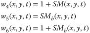
Quality metrics are composed of several stages. The last stage is called pooling. This stage aims at computing the final quality score from a 2D distortion (or error) map. For most saliency-based metrics [52–56], the use of the saliency map consists in modifying the pooling strategy. The degree of saliency of a given pixel is used as a weight, giving more or less importance to the error occurring on this pixel location.
The difference between these methods concerns the way the weights are defined. As presented in Ninassi et al. [53], different methods to compute the weights can be used:
11.4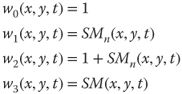
where ![]() is the unnormalized human saliency map,
is the unnormalized human saliency map, ![]() is the human saliency map normalized in the range
is the human saliency map normalized in the range ![]() , and
, and ![]() is a binarized human saliency map. The weighting function
is a binarized human saliency map. The weighting function ![]() is the baseline quality metrics in which the pooling is not modified. The functions
is the baseline quality metrics in which the pooling is not modified. The functions ![]() ,
, ![]() , and
, and ![]() give more importance to the salient areas than the others. The offset value of
give more importance to the salient areas than the others. The offset value of ![]() in the weighting functions
in the weighting functions ![]() ,
, ![]() , and
, and ![]() allows to take into account distortions also appearing on the non-salient areas.
allows to take into account distortions also appearing on the non-salient areas.
The use of a saliency map in the pooling stage provides contrasting results. In Reference [53], the use of a saliency map does not improve the performance of the quality metric. On the other hand, Akamine and Farias [56] showed that the performance of very simple metrics (Peak Signal to Noise-ratio (PSNR) and MSE) has been improved by the use of saliency information. However, for the SSIM metric [57], the saliency does not allow to improve the metric performance. In addition, they showed that the performance improvement depends on the saliency model used to generate the saliency map and on the distortion type (white noise, JPEG distortions).
Many authors working in this field consider that visual attention is important for assessing the quality of an image. However, there are still a number of open issues as demonstrated by Ninassi et al. [53, 56]. New strategies to incorporate visual attention into quality metrics as well as a better understanding of the interactions between saliency and distortion need to be addressed.
11.5 Conclusion
During the last two decades, significant progress has been made in the area of visual attention. Although the picture is much clearer, there are still a number of hurdles to overcome. For instance, the eye-tracking datasets used for evaluating the performance of computational models are more or less corrupted by biases. Among them, the central bias, which is the tendency of observers to look near the screen center, is probably the most important [24, 58]. The central bias, which is extremely difficult to cancel or to remove, is a fundamental flaw which can significantly undermine conclusions of some studies and the model's performance.
Regarding the applications, we are still in the early stages of use of saliency maps in computer vision applications. This is a promising avenue for improving existing image and video applications, and for the creation of new applications. Indeed, several factors are nowadays turning saliency computation from labs to industry:
· The models' accuracy has drastically increased in two decades, both concerning bottom-up saliency and top-down information and learning. The results of recent models are far better than the first results obtained in 1998.
· Models working both on videos and images are more and more numerous and provide more and more realistic results.
· The combined enhancement of computing hardware and algorithms optimization have led to real-time or almost real-time good-quality saliency computation.
While some industries have already begun to use attention maps (marketing), others (TV, multimedia) now make use of such algorithms. Video surveillance and video summarization will also enter the game of using saliency maps shortly. This move from labs to industry will further encourage research on the topic toward understanding human attention, memory, and human motivation.
References
1. 1. Findlay, J.M. (1997) Saccade target selection during visual search. Vision Res., 37, 617–631.
2. 2. Borji, A. and Itti, L. (2013) State-of-the-art in visual attention modeling. IEEE Trans. Pattern Anal. Mach. Intell., 35 (1), 185–207.
3. 3. Itti, L., Koch, C., and Niebur, E. (1998) A model for saliency-based visual attention for rapid scene analysis. IEEE Trans. Pattern Anal. Mach. Intell., 20, 1254–1259.
4. 4. Le Meur, O. and Le Callet, P. (2009) What we see is most likely to be what matters: visual attention and applications. ICIP, pp. 3085–3088.
5. 5. Treisman, A. and Gelade, G. (1980) A feature-integration theory of attention. Cognit. Psychol., 12 (1), 97–136.
6. 6. Koch, C. and Ullman, S. (1985) Shifts in selective visual attention: towards the underlying neural circuitry. Hum. Neurobiol., 4, 219–227.
7. 7. Wolfe, J.M. and Horowitz, T.S. (2004) What attributes guide the deployment of visual attention and how do they do it? Nat. Rev. Neurosci., 5 (6), 495–501.
8. 8. Le Meur, O., Le Callet, P., Barba, D., and Thoreau, D. (2006) A coherent computational approach to model the bottom-up visual attention. IEEE Trans. Pattern Anal. Mach. Intell., 28 (5), 802–817.
9. 9. Le Meur, O., Le Callet, P., and Barba, D. (2007) Predicting visual fixations on video based on low-level visual features. Vision Res., 47, 2483–2498.
10.10. Marat, S., Ho-Phuoc, T., Granjon, L., Guyader, N., Pellerin, D., and Guérin-Dugué, A. (2009) Modeling spatio-temporal saliency to predict gaze direction for short videos. Int. J. Comput. Vis., 82, 231–243.
11.11. Oliva, A., Torralba, A., Castelhano, M., and Henderson, J. (2003) Top-down control of visual attention in object detection. IEEE ICIP.
12.12. Mancas, M. (2007) Computational Attention Towards Attentive Computers, Presses University de Louvain.
13.13. Riche, N., Mancas, M., Duvinage, M., Mibulumukini, M., Gosselin, B., and Dutoit, T. (2013) Rare2012: a multi-scale rarity-based saliency detection with its comparative statistical analysis. Signal Process. Image Commun., 28 (6), 642–658, doi: http://dx.doi.org/10.1016/j.image.2013.03.009.
14.14. Bruce, N. and Tsotsos, J. (2009) Saliency, attention and visual search: an information theoretic approach. J. Vis., 9, 1–24.
15.15. Gao, D. and Vasconcelos, N. (2009) Bottom-up saliency is a discriminant process. ICCV.
16.16. Zhang, L., Tong, M.H., Marks, T.K., Shan, H., and Cottrell, G.W. (2008) SUN: a Bayesian framework for salience using natural statistics. J. Vis., 8 (7), 1–20.
17.17. Itti, L. and Baldi, P. (2005) Bayesian surprise attracts human attention. Neural Information Processing Systems.
18.18. Torralba, A., Oliva, A., Castelhano, M., and Henderson, J. (2006) Contextual guidance of eye movements and attention in real-world scenes: the role of global features in object search. Psychol. Rev., 113(4), 766–786.
19.19. Hou, X. and Zhang, L. (2007) Saliency detection: a spectral residual approach. IEEE Conf. on CVPR, 1–8.
20.20. Guo, C., Ma, Q., and Zhang, L. (2008) Spatio-temporal saliency detection using phase spectrum of quaternion Fourier transform. Computer Vision and Pattern Recognition, 1–8.
21.21. Guo, C. and Zhang, L. (2010) A novel multiresolution spatiotemporal saliency detection model and its application in image and video compression. IEEE Trans. Image Process., 19 (1), 185–198.
22.22. Garcia-Diaz, A., Fdez-Vidal, X.R., Pardo, X.M., and Dosil, R. (2012) Saliency from hierarchical adaptation through decorrelation and variance normalization. Image Vision Comput., 30 (1), 51–64, doi: http://dx.doi.org/10.1016/j.imavis.2011.11.007.
23.23. Harel, J., Koch, C., and Perona, P. (2006) Graph-based visual saliency. Proceedings of Neural Information Processing Systems (NIPS).
24.24. Le Meur, O. and Baccino, T. (2013) Methods for comparing scanpaths and saliency maps: strengths and weaknesses. Behav. Res. Methods, 1, 1–16.
25.25. Itti, L. (2000) Models of bottom-up and top-down visual attention. PhD thesis. California Institute of Technology.
26.26. Daly, S. (1993) Digital Images and Human Vision, MIT Press, Cambridge, MA, pp. 179–206.
27.27. Le Callet, P. (2001) Critères objectifs avec référence de qualité visuelle des images couleurs. PhD thesis. Université de Nantes.
28.28. Chamaret, C., Le Meur, O., and Chevet, J. (2010) Spatio-temporal combination of saliency maps and eye-tracking assessment of different strategies. ICIP, pp. 1077–1080.
29.29. Judd, T., Durand, F., and Torralba, A. (2012) A Benchmark of Computational Models of Saliency to Predict Human Fixations. Technical Report (CSAIL-TR-2012-001), MIT.
30.30. Foulsham, T., Kingstone, A., and Underwood, G. (2008) Turning the world around: patterns in saccade direction vary with picture orientation. Vision Res., 48, 1777–1790.
31.31. Judd, T., Ehinger, K., Durand, F., and Torralba, A. (2009) Learning to predict where people look. ICCV.
32.32. Le Meur, O. (2011) Predicting saliency using two contextual priors: the dominant depth and the horizon line. IEEE Int. Conf. on Multimedia and Expo ICME, 1–6.
33.33. Kim, Y., Varshney, A., Jacobs, D.W., and Guimbretière, F. (2010) Mesh saliency and human eye fixations. ACM Trans. Appl. Percept., 7 (2), 1–13.
34.34. Song, R., Liu, Y., Martin, R.R., and Rosin, P.L. (2014) Mesh saliency via spectral processing. ACM Trans. Graph., 33 (1), 6:1–6:17, doi: 10.1145/2530691.
35.35. DeCarlo, D. and Santella, A. (2002) Stylization and abstraction of photographs. ACM Trans. Graph., 21 (3), 769–776, doi: 10.1145/566654.566650.
36.36. Li, Z., Qin, S., and Itti, L. (2011) Visual attention guided bit allocation in video compression. Image Vision Comput., 29 (1), 1–14.
37.37. Liu, Z., Zou, W., and Le Meur, O. (2014) Saliency tree: a novel saliency detection framework. IEEE Trans. Image Process., 23 (5), 1937–1952.
38.38. Liu, Z., Zhang, X., Luo, S., and Le Meur, O. (2014) Superpixel-based spatiotemporal saliency detection. IEEE Trans. Circ. Syst. Video Technol., doi: 10.1109/TCSVT.2014.23086422014.2308642.
39.39. Isola, P., Xiao, J., Torralba, A., and Oliva, A. (2011) What makes an image memorable?. IEEE Conference on Computer Vision and Pattern Recognition (CVPR), pp. 145–152.
40.40. Khosla, A., Xiao, J., Torralba, A., and Oliva, A. (2012) Memorability of image regions. Advances in Neural Information Processing Systems (NIPS), Lake Tahoe, CA, USA.
41.41. Mancas, M. and Le Meur, O. (2013) Memorability of natural scene: the role of attention. ICIP.
42.42. Standing, L. (1973) Learning 10,000 pictures. Q. J. Exp. Psychol., 25, 207–222.
43.43. Tatler, B., Baddeley, R.J., and Gilchrist, I. (2005) Visual correlates of fixation selection: effects of scale and time. Vision Res., 45, 643–659.
44.44. Carmi, R. and Itti, L. (2006) Visual causes versus correlates of attentional selection in dynamic scenes. Vision Res., 46 (26), 4333–4345.
45.45. Oliva, A. and Torralba, A. (2001) Modeling the shape of the scene: a holistic representation of the spatial envelope. Int. J. Comput. Vision, 42 (3), 145–175.
46.46. Lazebnik, S., Schmid, C., and Ponce, J. (2006) Beyond bags of features: spatial pyramid matching for recognizing natural scene categories. 2006 IEEE Computer Society Conference on Computer Vision and Pattern Recognition, vol. 2, IEEE, pp. 2169–2178.
47.47. Dalal, N. and Triggs, B. (2005) Histograms of oriented gradients for human detection. IEEE Computer Society Conference on Computer Vision and Pattern Recognition, 2005. CVPR 2005, vol. 1, IEEE, pp. 886–893.
48.48. Shechtman, E. and Irani, M. (2007) Matching local self-similarities across images and videos. IEEE Conference on Computer Vision and Pattern Recognition, 2007. CVPR'07, IEEE, pp. 1–8.
49.49. Celikkale, B., Erdem, A., and Erdem, E. (2013) Visual attention-driven spatial pooling for image memorability. 2013 IEEE Computer Society Conference on Computer Vision and Pattern Recognition Workshops (CVPRW), IEEE, pp. 1–8.
50.50. Le Meur, O., Ninassi, A., Le Callet, P., and Barba, D. (2010) Overt visual attention for free-viewing and quality assessment tasks: impact of the regions of interest on a video quality metric. Signal Process. Image Commun., 25 (7), 547–558.
51.51. Le Meur, O., Ninassi, A., Le Callet, P., and Barba, D. (2010) Do video coding impairments disturb the visual attention deployment? Signal Process. Image Commun., 25 (8), 597–609.
52.52. Ninassi, A., Le Meur, O., Le Callet, P., and Barba, D. (2007) Does where you gaze on an image affect your perception of quality? Applying visual attention to image quality metric, ICIP. 169–172.
53.53. Ninassi, A., Le Meur, O., Le Callet, P., and Barba, D. (2009) Considering temporal variations of spatial visual distortions in video quality assessment. IEEE J. Sel. Top. Signal Process., 3 (2), 253–265.
54.54. Liu, H. and Heynderickx, I. (2011) Visual attention in objective image quality assessment: based on eye-tracking data. IEEE Trans. Circ. Syst. Video Technol., 21 (7), 971–982.
55.55. Guo, A., Zhao, D., Liu, S., Fan, X., and Gao, W. (2011) Visual attention based image quality assessment. IEEE International Conference on Image Processing, pp. 3297–3300.
56.56. Akamine, W.Y.L. and Farias, M.C.Q. (2014) Incorporating visual attention models into image quality metrics. Proc. SPIE-IS&T Electronic Imaging, 9016,90160O-1-9.
57.57. Wang, Z., Bovik, A.C., Sheikh, H.R., and Simoncelli, E. (2004) Image quality assessment: from error visibility to structural similarity. IEEE Trans. Image Process., 13 (4), 600–612.
58.58. Tatler, B.W. (2007) The central fixation bias in scene viewing: selecting an optimal viewing position independently of motor biases and image feature distributions. J. Vis., 7 (14), 4.1–417.