Biologically Inspired Computer Vision (2015)

Part III
Modelling

Chapter 13
Cortical Networks of Visual Recognition

Christian Thériault, Nicolas Thome and Matthieu Cord

13.1 Introduction

Human visual recognition is a far from trivial feat of nature. The light patterns projected on the human retina are always changing, and an object will never create exactly the same pattern twice. Objects move and transform constantly, appearing under unlimited number of aspects. Yet, the human visual system can recognize objects in milliseconds. It is thus natural for computer vision models to draw inspiration from the human visual cortex.

Most of what is understood about the visual cortex, and particularly about how it is able to achieve object recognition, comes from neurophysiological and psychophysical studies. A global picture emerges from over six decades of studies – the visual cortex is mainly organized as a parallel and massively distributed network of self-repeating local operations. Neurophysiological data and models of cortical circuitry have shed light on the processes by which feedforward (bottom-up) activation can generate early neural response of visual recognition [1, 2]. Contextual modulation and attentional mechanisms, through lateral and cortical feedback (top-down) connections, are clearly essential to the full visual recognition process [3–8]. Nevertheless, basic feedforward models [9–11] without feedback connections already display interesting levels of recognition, and provide a simple design around which the full functioning of the visual cortex can be studied. The circuitry of the visual cortex has also been studied in the language of differential geometry, which provides a natural connection between local neural operations, global activation, and perceptual phenomena [12–16].

This chapter introduces basic concepts on visual recognition by the cortex and some of its models. The global organization of the visual cortex is presented in Section 13.2. Local operations are followed in Section 13.4 by a special emphasis on operations in the primary visual cortex. Object recognition models are presented in Section 13.5, with a detailed description of a general model in Section 13.6. Section 13.7 focuses on a mathematical abstraction which corresponds to the structure of the primary visual cortex and which provides a model of contour emergence. Section 13.8 presents psychophysical and biological bases supporting such a model. The importance of feedback connections is discussed in Section 13.9, and the chapter concludes with the role of transformations (i.e., motion) in learning-invariant representations of objects.

13.2 Global Organization of the Visual Cortex

The brain is a dynamical system in which specialized areas receive and send connections to other multiple areas – brain functions emerge from the interaction of subpopulations of specialized neurons. As illustrated in Figure 13.1, the visual cortex makes no exception, and contains interacting subpopulations of neurons tuned to process visual information (shape, color, motion, etc.).

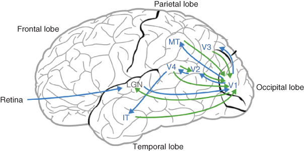
Figure 13.1 Basic organization of the visual cortex. Arrows illustrate the connections between various specialized subpopulations of neurons. Green and blue arrows indicate feedback and feedforward connections, respectively. The lateral geniculate nucleus (LGN), an extracortical area, is represented in gray.

The laminar structure of the cortex enables researchers to distinguish between lateral connections inside each area, feedback connections between areas, and feedforward connections streaming up from retinal inputs [17]. Up to now, the two most studied cortical visual areas have been the V1 area, the first area receiving extracortical inputs from the lateral geniculate nucleus (LGN), and the V5/MT (medial temporal) area.

A general consensus is that neurons in V1 behave as spatiotemporal filters, selective to local changes in color, spatial orientations, spatial frequencies, motion direction, and speed [18, 19]. The V5/MT area shares connections with V1 and also contains populations of neurons sensitive to motion speed and direction (see Chapter 12). Its contribution to motion perception beyond what is already observed in V1 is still not fully determined [20] and may involve the processing of motion over a broader range of spatiotemporal patterns compared to V1 [18, 21, 22].

Beginning at V1, there are interacting streams of visual information – the ventral pathway, which begins at V1 and goes into the temporal lobe, and the dorsal pathway, which also begins at V1 but goes into the parietal lobe [23]. The latter is traditionally associated with spatial information (i.e., “where”) while the former is traditionally associated with object recognition (i.e., “what”). However, mounting evidence indicates significant connections between the two pathways and the dynamics of their interaction is now recognized [17, 24–27].

Feedforward activation in the ventral pathway is correlated with the rapid (i.e., 100–200 ms) ability of humans to recognize visual objects [1, 28], but recurrent feedback activity between these areas should not be ruled out, even during rapid recognition [29]. The role of later stages beyond V1, (i.e., V2, V3, and V4) remains less understood, although neurons in the IT (inferior temporal) area have been shown to respond to more complex and global patterns, independently of spatial position and pose (i.e., full objects, faces, etc.) [1, 23].

13.3 Local Operations: Receptive Fields

Neurons in the visual cortex follow a retinotopic organization – local regions of the visual field, called receptive fields, are mapped to corresponding neurons [30]. In some areas, such as V1, the retinotopic mapping is continuous [31] – adjacent neurons have adjacent overlapping receptive fields. At different stages in the visual pathway, neurons have receptive fields which vary in size and complexity [23]. As presented in Section 13.4, neurons in V1 respond to local changes (i.e., the derivative of light intensity) over orientations and spatiotemporal frequencies. These small, local, receptive fields are integrated into larger receptive fields by neurons in the later stages of the V1IT pathway (Figure 13.2). This gives rise to representations of more complex patterns along the pathway, such as in the V4 [32, 33]. In the later stages, such as the IT area, neurons have receptive sizes which cover the entire visual field andrespond to the identity of objects rather than their position [1, 34].

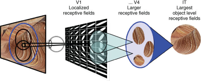
Figure 13.2 Receptive field organization. Neurons along the visual pathway V1IT have receptive fields which vary in size and complexity.

13.4 Local Operations in V1

Together with the work of Ref. [35], neurophysiological studies [36–38] have established a common finding about the spatial domain profile of receptive fields in the V1 area. This visual area is organized into a tilling of hypercolumns, in which the columns are composed of cells sensitive to spatial orientations with ocular dominance. Brain imaging techniques [39] have since revealed that orientation columns are spatially organized into a pinwheel crystal as illustrated in Figure 13.3.

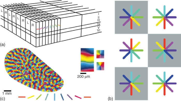
Figure 13.3 Primary visual cortex organization. (a) Hypercolumn structure showing the orientation and ocular dominance axes (image reproduced from Ref. [40]). (b) Idealized crystal pinwheel organization of hypercolumns in visual area V1 (image taken from Ref. [14]). (c) Brain imaging of visual area V1 of the tree shrew showing the pinwheel organization of orientation columns (image adapted from Ref. [39]).

Cells inside orientation columns are referred to as simple cells. In Chapter 14, the conditions under which the profile of simple cells naturally emerge from unsupervised learning are presented. The profile of simple cells can be modeled by Gaussian-modulated filters – Gaussian derivatives [41, 42] or Gabor filters [43–45]. Gaussian derivatives describe the V1 area in terms of differential geometry [41], whereas Gabor filters present the V1 area as a spatiotemporal frequency analyzer [37, 46]. Both filters are mathematically equivalent and differ mostly in terminology. As illustrated in Figure 13.4, the first- and second-order Gaussian derivatives give good approximations of Gabor filters with odd and even phase, respectively. In fact, Gaussian derivatives are asymptotically equal (for high-order derivatives) to Gabor filters [41]. The one-dimensional profile for the Gaussian derivatives and the (odd-phase) Gabor filter are respectively given by

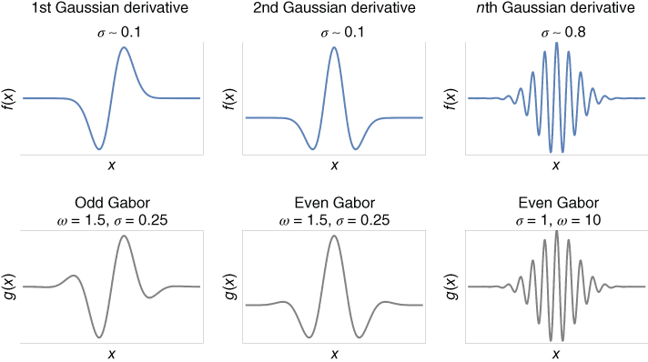
Figure 13.4 One-dimensional simple cell profiles. The curves shown are the graphs of local operators modeling the sensitivity profile of neurons in the primary visual cortex. Gabor filter and Gaussian derivative are local approximations of each other and are asymptotically equivalent for high-order of differentiation.

13.1

where is the Gaussian envelope of scale , and where gives the spatial frequency of the Gabor filter. In Reference [47], derivatives are further normalized with respect to to obtain scale invariance – filters at different scales will give the same maximum output. The even-phase Gabor filters is simply defined by a cosine function instead of a sine function. In Reference [42], cortical receptive field with order of differentiation as high as are reported, with the vast majority being .

Two-dimensional filters for the first-order Gaussian derivative and the odd-phase Gabor are respectively given by

13.2

where the Gaussian envelope is . For and , the filters and correspond to a rotation of the axes through an angle at scale , and model the orientation selectivity of simple cells in the hypercolumns. Specifically, when applied to an image , the Gaussian derivative gives the directional derivative, in the direction , of the image smoothed by the Gaussian at scale

13.3

where denotes the convolution product. The odd-phase Gabor gives the same directional derivative up to a multiplicative constant. Figure 13.5 illustrates examples of first-order Gaussian derivatives and even-phase Gabor filters at various scales and orientations. When representing cell activations in V1, the outputs of these filters can then be propagated synchronously or asynchronously [48] through a multilayer architecture simulating the basic feedforward principles of the visual cortex, as in Section 13.6.

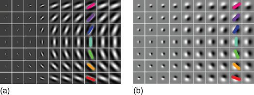
Figure 13.5 Two-dimensional simple cell profiles. The figure illustrates two-dimensional Gabor filters (a) and first-order Gaussian derivatives (b) at various scales and orientations. Colors can be put in relation to Figure 13.3.

Neurophysiological studies also identified complex cells in the V1V4 pathway. These cells also respond to specific frequencies and orientations, but their spatial sensitivity profiles are not localized as with simple cells, as illustrated in Figure 13.6. Complex cells display invariance (tolerance) to the exact position of the visual patterns at the scale of the receptive field. By allowing local shifts in the exact position of patterns, they may play a role in our ability to recognize objects invariantly with respect to transformations. Complex cells can be modeled by a MAX or soft-MAX operations applied to incoming simple cells [49]. Section 13.6 presents a model of such simple and complex cells network using the MAX operation in a multilayer architecture.

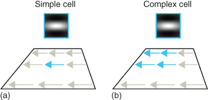
Figure 13.6 Complex cells. (a) The simple cell responds selectively to a local spatial derivative (blue arrow). (b) The complex cell responds selectively to the same spatial pattern, but displays invariance to its exact position. Complex cells are believed to gain their invariance by integrating (summing) over simple cells of the same selectivity.

13.5 Multilayer Models

On the basis of the above considerations, the vast majority of biologically inspired models are multilayer networks where the layers represent the various stages of processing corresponding to physiological data obtained about the mammalian visual pathways.

For most multilayer networks, the first layers are modeled by the operations of simple cells and complex cells in the primary visual cortex V1, as presented in the preceding section. However, the bulk of neurophysiological data clearly indicate important areas for visual recognition beyond area V1. These stages of processing are less understood. Multilayer networks usually model these stages with a series of layers which generate increasing complexity and invariance of representations [9, 11] (Figure 13.7). These representations are most often learned from experience by defining learning rules which modify the connections between layers.

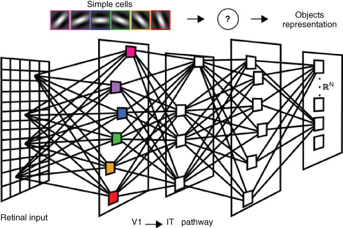
Figure 13.7 Multilayer architecture. The cortical visual pathway is usually modeled by multilayer networks. Synaptic connections for the early stages, such as V1 (first layer), are usually sensitive to local changes in spatial orientations and frequencies. Connections in the latter stages is an active research topic.

Supervised learning can be used with the objective to minimize error in object representations while retaining some degree of invariance to basic visual transforms [50, 51]. Networks using supervised learning are most often based on the error gradient backpropagation through the layers [52].

Unsupervised learning uses statistical regularities of the visual world to learn useful representations. One basic principle is to use temporal correlations between views of a transforming object. The hypothesis, in this case, is that we do not change the world by moving in it. Stated differently, neural representations should change on a slower timescale than the retinal input [53]. Such networks [23, 54, 55] are often based on the so called trace rule which minimizes variations of neural response to objects undergoing transformations. Other authors [48] have shown that the temporal aspect of neural spikes across layers can be used to define unsupervised learning of relevant object features. Unsupervised learning has also been used in generative models to find the appropriate representation space for each layer as the initial condition for supervised learning [56, 57].

13.6 A Basic Introductory Model

A simple and efficient model of the basic feedforward mechanisms of the visual pathway V1IT is given by the HMAX network and its variations [9–11]. In its most basic form, this network does not model full connectivity of the visual cortex, for instance, long-range horizontal connections described in the next section – the basic HMAX model is in essence a purely feedforward network. Nevertheless, it is based on hypercolumn organization and provides a starting point to model the visual cortical pathway.

The layers of the HMAX model are decomposed into parallel sublayers called feature maps. The activation of one feature map corresponds to the mapping of one filter (one feature) at all positions of the visual field. On the first layer, the features are defined by the outputs of simple cells given by Eq. (13.1). Each simple cell calculates a directional derivative and corresponds geometrically to an orientation and an amplitude (i.e., a vector). The feature maps on the first layer of the HMAX are therefore vector fields, corresponding to cross sections of the hypercolumns in V1 – the selection of one directional derivative per position is, by definition, a vector field expressing the local action of a transformation.

As illustrated in Figure 13.8, the first layer in HMAX enables the expression of various group actions, particularly those corresponding to basic transformations imposed on the retinal image, for which visual recognition is known to be invariant. Pooling over the parameters of a transformation group (i.e., pooling over translations) generates representations which are invariant to such transformation [58]. In the basic HMAX, mapping and pooling over translation fields of multiple orientations gives the model some degree of invariance to local translations, and consequently to shape deformations.

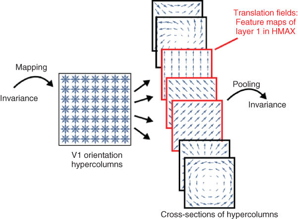
Figure 13.8 Sublayers in HMAX. The figure illustrates cross sections of the orientation hypercolumns in V1. Each cross section selects one simple cell per position, thereby defining a vector field. The first layer of HMAX is composed of sublayers defining translation fields (that is, the same orientation at all positions). By pooling over translation fields at various orientations, the HMAX model displays tolerance to local translations, which results in degrees of invariance to shape distortions. For illustration, the figure shows the image of the word Invariance, with its component translated. By pooling the local maximum values of translation fields mapped onto the image, the HMAX model tolerates local translations, and will produce a representation which is invariant to those local transformations.

The overall HMAX model follows a series of convolution/pooling steps as in Refs [9, 59] and illustrated in Figure 13.9. Each convolution step yields a set of feature maps and each pooling step provides tolerance (invariance) to variations in these feature maps. Each step is detailed below.

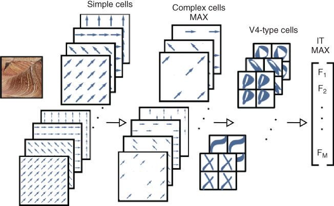
Figure 13.9 General HMAX network. The network alternates layers of feature mapping (convolution) and layers of feature pooling (MAX function). The convolution layers generate specific feature information, whereas the pooling layers results in degrees of invariance by relaxing the configuration of these features.

Layer 1 (simple cells). Each feature map is activated by the convolution of the input image with a set of simple cell filters with orientations and scales as defined in Eq. (13.2). Given an image , Layer 1 at orientation and scale is given by the absolute value of the convolution product

13.4

The layer can further be self-organized [60] through a process called lateral inhibition which appears throughout the cortex. Lateral inhibition is the process by which a neuron suppresses the activation of its neighbors through inhibitory connections. This competition between neurons creates a form of refinement or sharpening of the signal by filtering out components of smaller amplitude relative to their surroundings. It is also considered as a biological mechanism for neural sparsity and corresponds to a subtractive normalization [61]. Sparse neural firing has been shown to improve the original HMAX architecture on classification simulations [62]. The effect of inhibitory connections between neighboring neurons can be implemented by taking the convolution product of maps in layer 1 with the filter defined in Eq. (13.5) – an inhibitory surround with an excitatory center. A form of divisive normalization [63, 64] can also be used (see layer 3, below). More refinement can be obtained by applying inhibition (or suppressing) the weaker orientations at each position [10, 11]. This can be accomplished by a one-dimensional version of the lateral inhibition filter (Figure 13.10) in Eq. (13.5).

13.5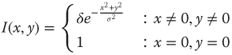

where defines the width of inhibition and defines the contrast.

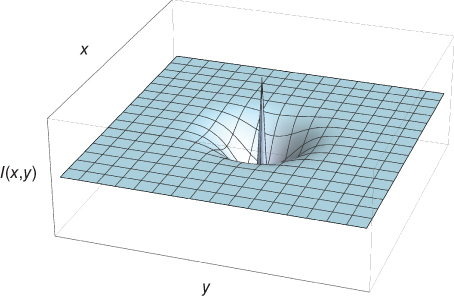
Figure 13.10 Lateral inhibition filter. A surround inhibition and an excitatory center.

Layer 2 (complex cells). Each feature map models the operations of complex cells in the visual cortex, illustrated in Figure 13.6. The output of complex cell selects the maximum value on a local neighborhood of simple cells. Maximum pooling over local neighborhoods results in invariance to local translations and thereby to global deformations [50] – it provides elasticity (illustrated in Figure 13.8) to the configuration of features of layer 1. Specifically, the second layer partitions each map into small neighborhoods and selects the maximum value inside each such that

13.6

Some degree of local scale invariance is also achieved by keeping only the maximum output over two adjacent scales at each position .

Layer 3 (V4-type cells). Layer at scale is obtained by applying filters to layer 2.

13.7

Each filter represents a V4-type cell – a configuration of multiple orientations representing more elaborated visual patterns than simple cells. In Reference [11], the also cover multiple scales, which give each filter the possibility of responding selectively to more complex patterns.

To implement a form of divisive normalization [63], the filters, and their input, can be normalized to unit length. This normalization will ensure that only the geometrical aspect of the inputs are considered, and not the contrast or the luminance level. The filters are learned from training images by sampling subsets of layer . This simple learning procedure consists in sampling subparts of layer and storing them as the connections weights of the filters . The training procedure, as done in Ref. [11], is illustrated in Figure 13.11. In the figure, a local subset of spatial size is selected from layer . The sample covers all orientations and a range of scales . To make the filter more selective, one possibility is to keep only the strongest coefficient in scales and orientations at each position, setting all other coefficients to zero. This sampling is repeated for a total of filters. In Reference [58], it is shown that for a system invariant to various geometrical transformations, such as the HMAX, this type of learning requires fewer samples in order to display classification properties.

Figure 13.11 V4-type cells. On layer 3, the cells represent configurations of complex cells, of various orientations and scales, sampled during training. The ellipses represent the receptive fields of simple cells on the first layer.

Layer 4 (IT-like cells). To gain global invariance, and to represent patterns of neural activation in higher visual areas such as IT, the final representation is activated by pooling the maximum output of across positions and scales. Pooling over the entire visual space, spatially and over all scales, guarantees invariance to position and size. However, important spatial and scale information for recognition might be lost by such global pooling.

In Reference [11], to maintain some spatial and scale information in the final representation, a set of concentric pooling regions is established around the spatial position and the scale at which each filter was sampled during training. As shown in Figure 13.12, each pooling region is defined by a radius centered on the training position and covers scales in the range .

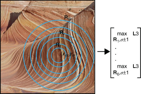
Figure 13.12 Multiresolution pooling. The training spatial position and scale of each filter is stored during training. For each new image, concentric pooling regions are centered on this coordinate. The maximum value is pooled from each pooling radius and across scales . This ensures that some spatial and scale information are kept in the final representation.

This pooling procedure is applied for all filters and the results are concatenated into a final vector representation (Eq. (13.8)). Each element of the vector represents the maximum activation level of each filter inside each search region. One hypothesis discussed in Ref. [1] is that local selectivity, combined with invariant pooling, may be a general principle by which the cortex performs visual classification. A combination of selectivity and invariance (i.e., relaxation of spatial configurations by maximum pooling), gained locally on each layer of the network, progressively maps the inputs to a representation space (i.e., a vector space), where the visual classes are more easily separable – where the class manifolds are untangled. As such, the final vector representation of Eq. (13.8) generates a space inside which classification of complex visual inputs can be performed relatively well with a vector classifier [11].

13.8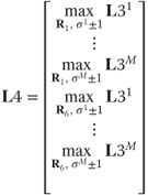

The operations of layer 1 of the basic HMAX network presented above is a highly simplified, and not entirely faithful, model of the hypercolumns' organization in the primary visual cortex. For one, the actual hypercolumns' structure is not explicitly represented, it is only implied by its decomposition into translation vector fields at multiple orientations. Also, there are no long-range horizontal connections between the hypercolumns corresponding to known neurophysiological data. The next section presents an idealized mathematical model of V1 which represents the hypercolumns explicitly. This model gives the hypercolumns of V1 a one-to-one correspondence with a mathematical structure and gives a formal expression of its horizontal connections.

13.7 Idealized Mathematical Model of V1: Fiber Bundle

There exists a mathematical model of visual area V1 which gives a theoretical formulation of the way the local operations of simple cells defined by Eq. (13.2) can merge into global percepts, and more precisely, into visual contours. As seen in the previous section, the HMAX is founded on a simplified model of the hypercolumns of V1. However, neurophysiological studies have clearly identified the important role, in the perception of shapes, of horizontal long-range connections between the hypercolumns [65]. When taken individually, the hypercolumns define the local orientations in the visual field. But how can these local orientationsdynamically interact such that a global percept emerges? The language of differential geometry provides a natural answer to this question. Indeed, there is a mathematical structure which, at a certain level, gives an abstraction of the physical structure of the primary visual cortex. It also provides, in the spirit of Gestalt psychology, a top-down definition of the way global shapes are generated by the visual system (Figure 13.13).

Figure 13.13 Contour completion. Understanding the principles by which the brain is able to spontaneously generate or complete visual contours sheds light on the importance of top-down and lateral processes in shape recognition (image reproduced from Ref. [66]).

To understand the abstract model of V1 described below, one can first note the similarity between the retinotopic organization of overlapping receptive fields on the retinal plane and the mathematical structure of a differentiable manifold – a smooth structure which locally resembles the Euclidean plane . One can also note that the repetition of hypercolumns in V1 provide a copy of the space of orientations over each position of the retinal plane. As introduced in the seminal work of Hoffman [12, 67, 68] and illustrated in Figure 13.14, this structure is the physical realization of a fiber bundle.

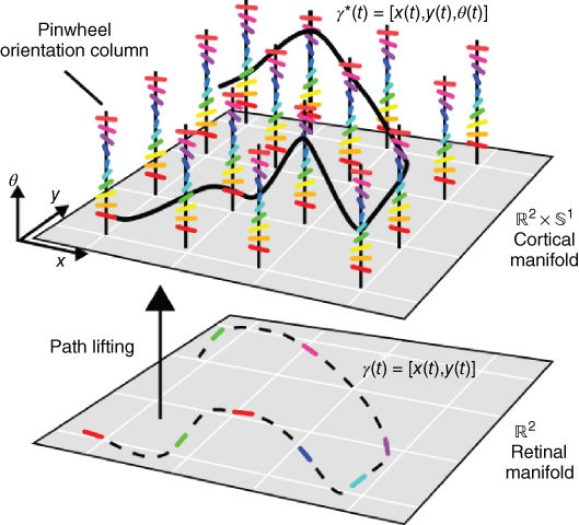
Figure 13.14 A fiber bundle abstraction of V1. Contour elements (dotted line) on the retinal plan () are lifted in the cortical fiber bundle () by making contact with simple cells (figure inspired from Refs [16, 40]).

A fiber bundle is a manifold on which is attached, at every position, the entire copy of another manifold called the fiber . The analogy with the visual cortex is direct – is the retinal plane and the fibers are the hypercolumns of simple cells. If simple cells are directional derivatives (Eq. (13.3)), then all orientations are distinguishable, and V1 is abstracted as [15, 16, 40, 69] where corresponds to the retinal plane, and where the unit circle corresponds to the group of rotations in the plane. This fiber bundle, also called the unit tangent bundle, is isomorphic to the Euclidean motion group SE(2), also called the Roto-translation group. If the simple cells are second-order derivatives (i.e., even-phase Gabors), then only the angles are distinguishable, and V1 is represented by , where is the space of all lines through the origin [70].

As illustrated in Figure 13.14, when a visual contour, expressed as a regular parameterized curve , makes contact with the simple cells, it is lifted in the hypercolumns to a curve . In the new space , the orientations are explicitly represented. Because of this, the problem of contour representation and contour completion in V1 is different than if it is expressed directly on the retinal image. Indeed, the type of curves in that can represent visual contours is very restricted. Every curve on the retinal plane corresponds to a lifted curve in , but the converse is not true – only special curves in can be curves in . For instance, the reader can verify that a straight line in is not a curve in . The Frobenius integrability theorem says that for a curve in to be a curve in we must have

13.9

It follows that it is admissible for a curve in V1 to represent a visual contour only if condition 13.9 is satisfied. Admissible curves in , illustrated in Figure 13.15, can be defined as the family of integral curves of , where

13.10

are vector fields generating a space in which is orthogonal to the directional derivative expressed by simple cells (Eq. (13.2)), and where gives the curvature of the curve projected on the retinal plane [15, 40].

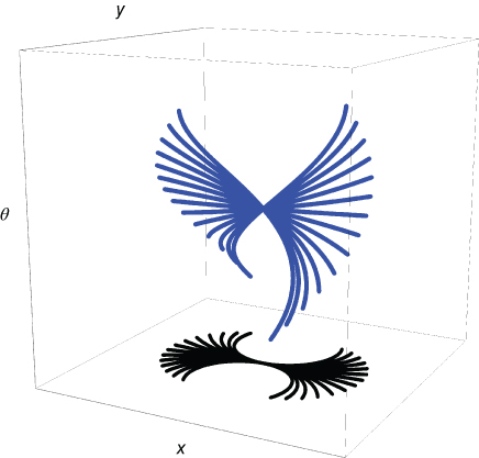
Figure 13.15 Family of integral curves in V1. The figure shows admissible V1 curves projected (in blue) on the retinal plane over one hypercolumn in (image adapted from Ref. [40]).

In References [15, 40], individual points at each hypercolumn are connected into global curves through the fan of integral curves, which together give a model of the lateral connectivity in V1, described in Section 13.8. This pattern of connectivity over the columns of V1 is illustrated in Figure 13.16.

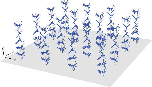
Figure 13.16 Horizontal connections. The fan of integral curves of the vector fields defined by Eq. (13.10) gives a connection between individual hypercolumns. It connects local tangent vectors at each hypercolumn into global curves (image adapted from Ref. [40]).

In References [16, 69], following earlier works [71–73], contour completion of the type shown in Figure 13.13 is defined by selecting, among the admissible curves of Eq. (13.9), the shortest path (i.e., geodesic) in between two visible boundary points. This gives a top-down formalism for perceptual phenomena such as contour completion and saliency (pop-out). As suggested by Hoffman [12, 68], contour completion and saliency is more the exception than the rule in the visual world. When the premises of the Frobenius integrability theorem are not satisfied (when orientations of simple cells do not line up), texture is perceived instead of contours. In other words, contour formation is not possible in V1 when the above integrability condition is not satisfied – in this frequent situation, it is not a contour that is perceived, but a texture. Using these principles, Hoffman defines visual contours of arbitrary complexity as the integral curves of an algebra of vector fields (i.e., Lie algebra) satisfying the above integrability conditions.

Of particular interest is the fact that the integral curves defined above are shown to correspond with long-range horizontal connections on the visual cortex. These connections are known as the association field[65] of perceptual contours and are described in the next section.

13.8 Horizontal Connections and the Association Field

Neurophysiological studies have shown that the outputs of simple cells (i.e., the shape of the filters in Figure 13.5) are modulated by contextual spatial surrounding – the global visual field modulates the local responses through long-range horizontal feedback in the primary visual cortex [74, 75]. In particular, in Ref. [65], psychophysical results suggest that long-range connections exist between simple cells oriented along particular paths, as illustrated in Figure 13.17. These connections may define what is referred to as an association field – grouping (associating) visual elements according to alignment constraints on position and orientation. By selecting configurations of simple cells, the V4-type cells modeled in Section 13.6 share some relations with the association field. However, these configurations are not explicitly defined by principles of grouping and alignment. As shown in Refs [14, 15, 40], the association field can be put in direct correspondence with the integral curves (see Figure 13.15) of the cortical fields expressed by simple cells and may well be the biological substrate for perceptual contours and phenomena (i.e., Gestalt) such as illusory contours, surface fill-in, and contour saliency.

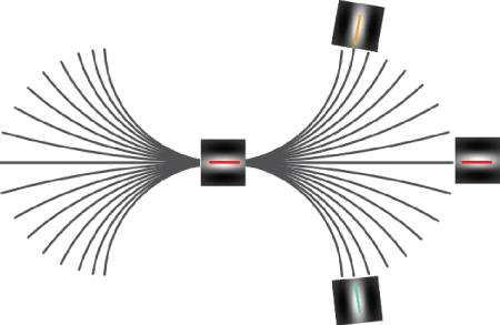
Figure 13.17 Association field. Long-range horizontal connections are the basis for the association field in Ref. [65]. The center of the figure represents a simple cell in V1. The curve displayed represents the visual path defined by the horizontal connections to other simple cells. The possible contours are shown to correspond to the family of integral curves as defined in Section 13.7, where the center cell gives the initial condition.

13.9 Feedback and Attentional Mechanisms

Studies also show that attentional mechanisms, regulated through cortical feedback, modulate neural processing in regions as early as V1. The spatial pattern of modulation in Ref. [76] reveals an attentional process which is consistent with an object-based attention window but is inconsistent with a simple circumscribed attentional processes. This study suggests that neural processing in visual area V1 is not only driven by inputs from the retina but is often influenced by attentional process mediated by top-down connections. Although rapid visual recognition has sometimes been modeled by purely feedforward networks (Section 13.6), studies and models [3] suggest that attentional mechanisms, mediated by top-down feedback, are essential for a full understanding of visual recognition mechanisms in the cortex. The question remains an open discussion, but it can be argued that there is indeed enough time for recurrent activation (feedback) to occur during rapid visual recognition (150 ms) [29]. For a description of bottom-up attentional visual models see Chapter 11.

13.10 Temporal Considerations, Transformations and Invariance

Object recognition may appear as a static process which involves the identification of visual inputs at one given instant. However, recognizing a visual object is everything but a static process and is fundamentally involved with transformations. The retinal image is never quite stable and visual perception vanishes in less than 80 ms in the absence of motion [77]. Ecologically speaking, invariance to transformations generated by motion is essential for visual recognition to occur, and transformations of the retinal image are present at every instant from birth. Self-produced movements, such as head and eyes movements, are correlated with transformations of the retinal image and must have profound effect on the neural coding of the visual field [78].

The involvement of motion in the perception of shapes is displayed clearly by phenomena such as structure from motion [79] and the segmentation of shapes from motion [20]. The connectivity of the visual cortex also suggests a role for motion in object recognition. The ventral pathway, traditionally associated with object recognition, and the dorsal pathway, often associated with motion perception and spatial localization, are known to be significantly interacting [26, 27].

In neural network modeling of visual recognition, motion and the temporal dimension of the neural response to an object undergoing transformations has been extensively modeled [23, 53, 54, 80, 81]. One unsupervised learning principle, common to all of these models, is to remove temporal variations in the neural response in the presence of transforming objects, as done by Mitchison [80] with a differential synapse. Another unsupervised learning rule based on the same principle is known as the trace rule [55]. This is a Hebbian learning rule which keeps a temporal trace of the neuron's output in response to a moving object passing inside its receptive field (see Figure 13.18). The inclusion of an activation trace in the learning rule drives neurons to respond invariantly to temporally close inputs (i.e., positions of a moving object). Inside an architecture with overlapping receptive fields, this allows a smooth mapping of transformations. This learning rule has also been used for the last layer of the HMAX model to gain translation invariance [81]. Interestingly, the trace learning rule can be mathematically related [82] to temporal difference (TD) learning [83], which minimizes TDs in response to successive inputs. For instance, one version of the trace learning rule modifies the connection weight vector of output neuron at time in response to input (Figure 13.18) such that

13.11

where is an exponential trace of the neuron's past activation.

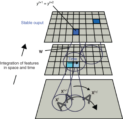
Figure 13.18 Temporal association. By keeping a temporal trace of recent activation, the trace learning rule enables neurons to correlate their activation with a transformation sequence passing through their receptive fields. This generates a neural response which is stable or invariant to transformation of objects inside their receptive fields.

A similar principle is also the basis of slow feature analysis [53] in which neurons learn to output a signal at a lower frequency than the incoming retinal signal, producing a stable response to transforming objects. The slow feature analysis has been integrated in the HMAX architecture in the context of recognition of dynamic scenes [84, 85]. The authors applied the slow feature analysis to the output of simple cells responding to image sequences in videos. This generates more stable representations of motion in comparison with the raw simple cell outputs. All these unsupervised learning rules, from the point of view of visual recognition, implicitly suggest that, for obvious ecological reasons, the identity of objects should not change because of relative motion between the observer and the objects, and that the brain uses spatiotemporal correlations in the signal to maintain a coherent representation.

13.11 Conclusion

The average number of synapses per neuron in the brain is close to 10,000, with a total estimate of 86 billion neurons in the human brain [86]. In particular, the primary visual cortex averages 140 millions neurons [87]. This roughly amounts to 1.4 trillion synaptic connections in and out of V1 alone. Interestingly, there is a large connection ratio between V1 and the retina. In particular, with an estimate of one million retinal ganglion cells [88], there is a connectivity ratio well over one hundred V1 neurons for each retinal ganglion cell.

With such massive connectivity, it is clear that the representation, the sampling, and the filtering (i.e., averaging) capacity of the visual cortex is far beyond neural network models which may be simulated on today's basic computers. The large number of V1 neurons allocated on each retinal fiber suggests a significant amount of image processing. For instance, the simple calculation of derivatives by the local operators defined in Eq. (13.2) is plagued with discretization noise when applied directly on pixelized images, unless very large images are used with a large Gaussian envelope defining the filters. This makes theoretical principles, such as differentiation, difficult to express in practice. It is tempting to suggest that visual cortex evolved with such an astronomical number of connections to deal with noise and irregularities of the visual world and to create a nearly smooth signal from the discretized retinal receptors. A massive number of horizontal connections between V1 cells, as presented in Sections 13.7 and 13.8, seem to be part of nature's solution to clean, segment, and amplify coherent visual structures in an otherwise cluttered environment.

Models such as the HMAX illustrate the basic functioning of simple and complex cells in V1. Without extensive horizontal and feedback connections, this model does not represent the full capacity of the visual cortical pathway. Nevertheless, it seems quite certain by now that one axiom of processing in V1 is based on local operations such as the ones described in Sections 13.4 and 13.6. A code for the model presented in Section 13.6 is available at http://www-poleia.lip6.fr/cord/Projects/Projects.html http://www-poleia.lip6.fr/cord/Projects/Projects.html. The next step in such a model could be to integrate feedback and horizontal connections, as defined in a more theoretical context in Section 13.7. It remains a challenge to implement such formal theoretical models on full-scale natural scenes. Research would most likely progress in the right direction by generating effort in bridging the gap between what is observed in the brain and models of visual recognition.

References

1. 1. DiCarlo, J.J., Zoccolan, D., and Rust, N.C. (2012) How does the brain solve visual object recognition? Neuron, 73, 415–434.

2. 2. Serre, T., Kouh, M., Cadieu, C., Knoblich, U., Kreiman, G., and Poggio, T. (2005) A Theory of Object Recognition: Computations and Circuits in the Feedforward Path of the Ventral Stream in Primate Visual Cortex. AI Memo 2005-036/CBCL Memo 259. Massachusetts Institute of Technology.

3. 3. Lee, T.S. and Mumford, D. (2003) Hierarchical Bayesian inference in the visual cortex. J. Opt. Soc. Am. A Opt. Image Sci. Vis., 20, 1434–1448.

4. 4. Borji, A. and Itti, L. (2013) State-of-the-art in visual attention modeling. IEEE Trans. Pattern Anal. Mach. Intell., 35 (1), 185–207.

5. 5. Itti, L. and Koch, C. (2001) Computational modelling of visual attention. Nat. Rev. Neurosci., 2 (3), 194–203.

6. 6. Siagian, C. and Itti, L. (2007) Rapid biologically-inspired scene classification using features shared with visual attention. IEEE Trans. Pattern Anal. Mach. Intell., 29 (2), 300–312.

7. 7. Zhang, Y., Meyers, E.M., Bichot, N.P., Serre, T., Poggio, T.A., and Desimone, R. (2011) Object decoding with attention in inferior temporal cortex. Proc. Natl. Acad. Sci. U.S.A., 108 (21), 8850–8855.

8. 8. Chikkerur, S., Serre, T., Tan, C., and Poggio, T. (2010) What and where: a Bayesian inference theory of attention. Vision Res., 50, 2233–2247.

9. 9. Serre, T., Wolf, L., Bileschi, S., Riesenhuber, M., and Poggio, T. (2007) Robust object recognition with cortex-like mechanisms. IEEE Trans. Pattern Anal. Mach. Intell., 29, 411–426.

10.10. Mutch, J. and Lowe, D.G. (2008) Object class recognition and localization using sparse features with limited receptive fields. Int. J. Comput. Vision, 80, 45–57.

11.11. Theriault, C., Thome, N., and Cord, M. (2013) Extended coding and pooling in the HMAX model. IEEE Trans. Image Process., 22 (2), 764–777.

12.12. Hoffman, W. (1989) The visual cortex is a contact bundle. Appl. Math. Comput., 32, 137–167.

13.13. Koenderink, J. (1988) Operational significance of receptive field assemblies. Biol. Cybern., 58, 163–171.

14.14. Petitot, J. (2003) The neurogeometry of pinwheels as a sub-Riemannian contact structure. J. Physiol. Paris, 97, 265–309.

15.15. Citti, G. and Sarti, A. (2006) A cortical based model of perceptual completion in the roto-translation space. J. Math. Imaging Vision, 24 (3), 307–326.

16.16. Ben-Yosef, G. and Ben-Shahar, O. (2012) A tangent bundle theory for visual curve completion. IEEE Trans. Pattern Anal. Mach. Intell., 34 (7), 1263–1280.

17.17. Felleman, D.J. and Essen, D.C.V. (1991) Distributed hierarchical processing in the primate cerebral cortex. Cereb. Cortex, 1 (1), 1–47.

18.18. Priebe, N.J., Lisberger, S.G., and Movshon, J.A. (2006) Tuning for spatiotemporal frequency and speed in directionally selective neurons of macaque striate cortex. J. Neurosci., 26 (11), 2941–2950.

19.19. Lennie, P. and Movshon, J. (2005) Coding of color and form in the geniculostriate visual pathway (invited review). J. Opt. Soc. Am. A Opt. Image Sci. Vis., 22, 2013–2033.

20.20. Born, R.T. and Bradley, D.C. (2005) Structure and function of visual area MT. Annu. Rev. Neurosci., 28 (1), 157–189.

21.21. Christopher, C.P., Richard, T.B., and Margaret, S.L. (2003) Two-dimensional substructure of stereo and motion interactions in macaque visual cortex. Neuron, 37, 525–535.

22.22. Pack, C.C. and Born, R.T. (2001) Temporal dynamics of a neural solution to the aperture problem in visual area MT of macaque brain. Nature, 409 (6823), 1040–1042.

23.23. Rolls, E. and Deco, G. (2002) Computational Neuroscience of Vision, 1st edn, Oxford University Press.

24.24. Cloutman, L.L. (2013) Interaction between dorsal and ventral processing streams: where, when and how? Brain Lang., 127 (2), 251–263.

25.25. Zanon, M., Busan, P., Monti, F., Pizzolato, G., and Battaglini, P. (2010) Cortical connections between dorsal and ventral visual streams in humans: evidence by TMS/EEG co-registration. Brain Topogr., 22 (4), 307–317.

26.26. Schenk, T. and McIntosh, R. (2010) Do we have independent visual streams for perception and action? Cogn. Neurosci., 1 (1), 52–62.

27.27. McIntosh, R. and Schenk, T. (2009) Two visual streams for perception and action: current trends. Neuropsychologia, 47 (6), 1391–1396.

28.28. Thorpe, S., Fize, D., and Marlot, C. (1996) Speed of processing in the human visual system. Nature, 381, 520–522.

29.29. Johnson, J.S. and Olshausen, B.A. (2003) Timecourse of neural signatures of object recognition. J. Vis., 3 (7), 499–512.

30.30. Hubel, D. (1962) The visual cortex of the brain. Sci. Am., 209 (5), 54–62.

31.31. Adams, D. and Horton, J. (2003) A precise retinotopic map of primate striate cortex generated from the representation of angioscotomas. J. Neurosci., 23 (9), 3371–3389.

32.32. Roe, A.W., Chelazzi, L., Connor, C.E., Conway, B.R., Fujita, I., Gallant, J.L., Lu, H., and Vanduffel, W. (2012) Toward a unified theory of visual area V4. Neuron, 14 (1), 12–29.

33.33. David, S.V., Hayden, B.Y., and Gallant, J.L. (2006) Spectral receptive field properties explain shape selectivity in area V4. J. Neurophysiol., 96 (6), 3492–3505.

34.34. Rolls, E.T., Aggelopoulos, N.C., and Zheng, F. (2003) The receptive fields of inferior temporal cortex neurons in natural scenes. J. Neurosci., 23, 339–348.

35.35. Hubel, D. and Wiesel, T. (1959) Receptive fields of single neurones in the cat's striate cortex. J. Physiol., 148, 574–591.

36.36. De Valois, R.L. and De Valois, K.K. (1988) Spatial Vision, Oxford Psychology Series, Oxford University Press, (1990 [printing]), New York, Oxford.

37.37. Maffei, L., Hertz, B.G., and Fiorentini, A. (1973) The visual cortex as a spatial frequency analyser. Vision Res., 13, 1255–1267.

38.38. Campbell, F.W., Cooper, G.F., and Cugell, E.C. (1969) The spatial selectivity of the visual cells of the cat. J. Physiol. (London), 203, 223–235.

39.39. Bosking, W., Zhang, Y., Schofield, B., and Fitzpatrick, D. (1997) Orientation selectivity and the arrangement of horizontal connections in tree shrew striate cortex. J. Neurosci., 17, 2112–2127.

40.40. Sanguinetti, G. (2011) Invariant models of vision between phenomenology, image statistics and neurosciences. PhD thesis. Universidad de la República, Facultad de Ingeniería, Uruguay.

41.41. Koenderink, J. and van Doorn, A. (1987) Representation of local geometry in the visual system. Biol. Cybern., 55, 367–375.

42.42. Young, R.A. (1987) The Gaussian derivative model for spatial vision: I. Retinal mechanisms. J. Physiol., 2, 273–293.

43.43. Gabor, D. (1946) Theory of communication. J. Inst. Electr. Eng., 93, 429–457.

44.44. Daugman, J.G. (1980) Two-dimensional spectral analysis of cortical receptive field profiles. Vision Res., 20 (10), 847–856.

45.45. Daugman, J.G. (1985) Uncertainty relation for resolution in space, spatial frequency, and orientation optimized by two-dimensional visual cortical filters. J. Opt. Soc. Am. A, 2 (7), 1160–1169.

46.46. Simoncelli, E. and Heeger, D. (1998) A model of neural responses in visual area MT. Vision Res., 38, 743–761.

47.47. Lindeberg, T. (1998) Feature detection with automatic scale selection. Int. J. Comput. Vision, 30, 77–116.

48.48. Masquelier, T. and Thorpe, S.J. (2007) Unsupervised learning of visual features through spike timing dependent plasticity. PLoS Comput. Biol., 3 (2), e31.

49.49. Lampl, I., Ferster, D., Poggio, T., Riesenhuber, M., Ferster, D., and Poggio, T. (2004) Intracellular measurements of spatial integration and the MAX operation in complex cells of the cat primary visual cortex. J. Neurophysiol., 92, 2704–2713.

50.50. Fukushima, K. and Miyake, S. (1982) Neocognitron: a new algorithm for pattern recognition tolerant of deformations and shifts in position. Pattern Recognit., 15 (6), 455–469.

51.51. Fukushima, K. (2003) Neocognitron for handwritten digit recognition. Neurocomputing, 51, 161–180.

52.52. Lecun, Y., Bottou, L., Bengio, Y., and Haffner, P. (1998) Gradient-based learning applied to document recognition. Proceedings of the IEEE, pp. 2278–2324.

53.53. Wiskott, L. and Sejnowski, T. (2002) Slow feature analysis: unsupervised learning of invariances. Neural Comput., 14, 715–770.

54.54. Rolls, E.T. and Milward, T.T. (2000) A model of invariant object recognition in the visual system: learning rules, activation functions, lateral inhibition, and information-based performance measures. Neural Comput., 12, 2547–2572.

55.55. Foldiak, P. (1991) Learning invariance from transformation sequences. Neural Comput., 3 (2), 194–200.

56.56. Vincent, P., Larochelle, H., Lajoie, I., Bengio, Y., and Manzagol, P.A. (2010) Stacked denoising autoencoders: learning useful representations in a deep network with a local denoising criterion. J. Mach. Learn. Res., 11, 3371–3408.

57.57. Goh, H., Thome, N., Cord, M., and Lim, J.H. (2012) Unsupervised and supervised visual codes with restricted Boltzmann machines. European Conference on Computer Vision (ECCV 2012).

58.58. Fabio, A., Joel, Z.L., Lorenzo, R., Jim, M., Andrea, T., and Poggio, T. (2014) Unsupervised Learning of Invariant Representations with Low Sample Complexity: The Magic of Sensory Cortex or a New Framework for Machine Learning? Technical Memo CBMM Memo No. 001, Center for Brains, Mind and Machines, MIT, Cambridge, MA.

59.59. Riesenhuber, M. and Poggio, T. (1999) Hierarchical models of object recognition in cortex. Nat. Neurosci., 2, 1019–1025.

60.60. Kohonen, T. (2001) Self-Organizing Maps, Springer Series in Information Sciences, vol. 30, 3rd edn, Springer-Verlag, Berlin.

61.61. Jarrett, K., Kavukcuoglu, K., Ranzato, M., and LeCun, Y. (2009) What is the best multi-stage architecture for object recognition? ICCV, IEEE, pp. 2146–2153.

62.62. Hu, X., Zhang, J., Li, J., and Zhang, B. (2014) Sparsity-regularized HMAX for visual recognition. PLoS ONE, 9 (1), e81 813.

63.63. Pinto, N., Cox, D.D., and DiCarlo, J.J. (2008) Why is real-world visual object recognition hard? PLoS Comput. Biol., 4 (1), e27.

64.64. Lyu, S. and Simoncelli, E.P. (2008) Nonlinear image representation using divisive normalization. CVPR, IEEE Computer Society.

65.65. Field, D.J., Hayes, A., and Hess, R.F. (1993) Contour integration by the human visual system: evidence for a local association field. Vision Res., 33, 173–193.

66.66. Thériault, C. (2006) Mémoire visuelle et géométrie différentielle : forces invariantes des champs de vecteurs élémentaires. PhD thesis. Université du Québec à Montréal.

67.67. Hoffman, W. (1966) The Lie algebra of visual perception. Math. Psychol., 3, 65–98.

68.68. Hoffman, W. (1970) Higher visual perception as prolongation of the basic Lie transformation group. Math. Biosci., 6, 437–471.

69.69. Ben-Yosef, G. and Ben-Shahar, O. (2012) Tangent bundle curve completion with locally connected parallel networks. Neural Comput., 24 (12), 3277–3316.

70.70. Petitot, J. and Tondut, Y. (1999) Vers une neurogéométrie. fibrations corticales, structures de contact et contours subjectifs modaux. Math. Sci. Hum., 145, 5–101.

71.71. Ullman, S. (1976) Filling-in the gaps: the shape of subjective contours and a model for their generation. Biol. Cybern., 25, 1–6.

72.72. Horn, B.K.P. (1983) The curve of least energy. ACM Trans. Math. Softw., 9 (4), 441–460.

73.73. Mumford, D. (1994) Elastica and computer vision, in Algebraic Geometry and its Applications (ed. C.L. Bajaj), Springer-Verlag, New York.

74.74. Gilbert, C.D., Das, A., and Westheimer, G. (1996) Spatial integration and cortical dynamics. Proc. Natl. Acad. Sci. U.S.A., 93, 615–622.

75.75. Bosking, W., Zhang, Y., Schofield, B., and Fitzpatrick, D. (1997) Orientation selectivity and the arrangement of horizontal connections in tree shrew striate cortex. J. Neurosci., 17 (6), 2112–2127.

76.76. Somers, D.C., Dale, A.M., and Tootell, R.B.H. (1999) Functional MRI reveals spatially specific attentional modulation in human primary visual cortex. Proc. Natl. Acad. Sci. U.S.A., 96, 1663–1668.

77.77. Coppola, D. and Purves, D. (1996) The extraordinarily rapid disappearance of entopic images. Proc. Natl. Acad. Sci. U.S.A., 93, 8001–8004.

78.78. Dodwell, P. (1983) The Lie transformation group of visual perception. Percept. Psychophys., 34, 1–16.

79.79. Grunewald, A., Bradley, D.C., and Andersen, R.A. (2002) Neural correlates of structure-from-motion perception in macaque V1 and MT. J. Neurosci., 22, 6195–6207.

80.80. Mitchison, G. (1991) Removing time variation with the anti-Hebbian differential synapse. Neural Comput., 3 (3), 312–320.

81.81. Isik, L., Leibo, J., and Poggio, T. (2012) Learning and disrupting invariance in visual recognition with a temporal association rule. Front. Comput. Neurosci., 6 (7), 37.

82.82. Rolls, E.T. and Stringer, S.M. (2001) Invariant object recognition in the visual system with error correction and temporal difference learning. Network, 12, 111–130.

83.83. Sutton, R.S. (1988) Learning to predict by the methods of temporal differences, in Machine Learning, Kluwer Academic Publishers, pp. 9–44.

84.84. Theriault, C., Thome, N., Cord, M., and Perez, P. (2014) Perceptual principles for video classification with slow feature analysis. J. Sel. Top. Signal Process., 8 (3), 428–437.

85.85. Theriault, C., Thome, N., and Cord, M. (2013) Dynamic scene classification: learning motion descriptors with slow features analysis. IEEE CVPR.

86.86. Azevedo, F.A.C., Carvalho, L.R.B., Grinberg, L.T., Farfel, J.M., Ferretti, R.E.L., Leite, R.E.P., Filho, W.J., Lent, R., and Herculano-Houzel, S. (2009) Equal numbers of neuronal and nonneuronal cells make the human brain an isometrically scaled-up primate brain. J. Comp. Neurol., 513 (5), 532–541.

87.87. Leuba, G. and Kraftsik, R. (1994) Changes in volume, surface estimate, three-dimensional shape and total number of neurons of the human primary visual cortex from midgestation until old age. Anat. Embryol., 190 (4), 351–366.

88.88. Curcio, C.A. and Allen, K.A. (1990) Topography of ganglion cells in human retina. J. Comp. Neurol., 300 (1), 5–25.