Biologically Inspired Computer Vision (2015)

Part III
Modelling

Chapter 14
Sparse Models for Computer Vision

Laurent U. Perrinet

14.1 Motivation

14.1.1 Efficiency and Sparseness in Biological Representations of Natural Images

The central nervous system is a dynamical, adaptive organ which constantly evolves to provide optimal decisions¹ for interacting with the environment. Early visual pathways provide with a powerful system for probing and modeling these mechanisms. For instance, the primary visual cortex of primates (V1) is absolutely central for most visual tasks. There, it is observed that some neurons from the input layer of V1 present selectivity for localized, edge-like features—as represented by their “receptive fields” [2]. Crucially, there is experimental evidence for sparse firing in the neocortex [3, 4] and in particular in V1. A representation is sparse when each input signal is associated with a relatively small subset of simultaneously activated neurons within a whole population. For instance, orientation selectivity of simple cells is sharper than the selectivity that would be predicted by linear filtering. Such a procedure produces a rough “sketch” of the image on the surface of V1 that is believed to serve as a “blackboard” for higher-level cortical areas [5]. However, it is still largely unknown how neural computations act in V1 to represent the image. More specifically, what is the role of sparseness—as a generic neural signature—in the global function of neural computations?

A popular view is that such a population of neurons operates such that relevant sensory information from the retinothalamic pathway is transformed (or “coded”) efficiently. Such efficient representation will allow decisions to be taken optimally in higher-level areas. In this framework, optimality is defined in terms of information theory [6–8]. For instance, the representation produced by the neural activity in V1 issparse: it is believed that this reduces redundancies and allows to better segregate edges in the image [9, 10]. This optimization is operated given biological constraints, such as the limited bandwidth of information transfer to higher processing stages or the limited amount of metabolic resources (energy or wiring length). More generally, it allows to increase the storage capacity of associative memories before memory patterns start to interfere with each other [11]. Moreover, it is now widely accepted that this redundancy reduction is achieved in a neural population through lateral interactions. Indeed, a link between anatomical data and a functional connectivity between neighboring representations of edges has been found by Bosking et al. [12], although their conclusions were more recently refined to show that this process may be more complex [13]. By linking neighboring neurons representing similar features, one allows thus a more efficient representation in V1. As computer vision systems are subject to similar constraints, applying such a paradigm therefore seems a promising approach toward more biomimetic algorithms.

It is believed that such a property reflects the efficient match of the representation with the statistics of natural scenes, that is, with behaviorally relevant sensory inputs. Indeed, sparse representations are prominently observed for cortical responses to natural stimuli [14–17]. As the function of neural systems mostly emerges from unsupervised learning, it follows that these are adapted to the inputs which are behaviorally the most common and important. More generally, by being adapted to natural scenes, this shows that sparseness is a neural signature of an underlying optimization process. In fact, one goal of neural computation in low-level sensory areas such as V1 is to provide relevant predictions [18, 19]. This is crucial for living beings as they are often confronted with noise (internal to the brain or external, such as in low light conditions), ambiguities (such as inferring a three dimensional slant from a bidimensional retinal image). In addition, the system has to compensate for inevitable delays, such as the delay from light stimulation to activation in V1 which is estimated to be of 50 ms in humans. For instance, a tennis ball moving at 20 m/s at 1 m in the frontal plane elicits an input activation in V1 corresponding to around 45° of visual angle behind its physical position [20]. Thus, to be able to translate such knowledge to the computer vision community, it is crucial to better understand why the neural processes that produce sparse coding are efficient.

14.1.2 Sparseness Induces Neural Organization

A breakthrough in the modeling of the representation in V1 was the discovery that sparseness is sufficient to induce the emergence of receptive fields similar to V1 simple cells [21]. This reflects the fact that, at the learning timescale, coding is optimized relative to the statistics of natural scenes such that independent components of the input are represented [22, 23]. The emergence of edge-like simple cell receptive fields in the input layer of area V1 of primates may thus be considered as a coupled coding and learning optimization problem: at the coding timescale, the sparseness of the representation is optimized for any given input while at the learning timescale, synaptic weights are tuned to achieve on average an optimal representation efficiency over natural scenes. This theory has allowed to connect the different fields by providing a link among information theory models, neuromimetic models, and physiological observations.

In practice, most sparse unsupervised learning models aim at optimizing a cost defined on prior assumptions on the sparseness of the representation. These sparse learning algorithms have been applied both for images [21, 24–29] and sounds [30, 31]. Sparse coding may also be relevant to the amount of energy the brain needs to use to sustain its function. The total neural activity generated in a brain area is inversely related to the sparseness of the code, therefore the total energy consumption decreases with increasing sparseness. As a matter of fact, the probability distribution functions of neural activity observed experimentally can be approximated by so-called exponential distributions, which have the property of maximizing information transmission for a given mean level of activity [32]. To solve such constraints, some models thus directly compute a sparseness cost based on the representation's distribution. For instance, the kurtosis corresponds to the fourth statistical moment (the first three moments being in order the mean, variance, and skewness) and measures how the statistics deviates from a Gaussian: a positive kurtosis measures whether this distribution has a “heavier tail” than a Gaussian for a similar variance—and thus corresponds to a sparser distribution. On the basis of such observations, other similar statistical measures of sparseness have been derived in the neuroscience literature [15].

A more general approach is to derive a representation cost. For instance, learning is accomplished in the SparseNet algorithmic framework [22] on image patches taken from natural images as a sequence of coding and learning steps. First, sparse coding is achieved using a gradient descent over a convex cost. We will see later in this chapter how this cost is derived from a prior on the probability distribution function of the coefficients and how it favors the sparseness of the representation. At this step, the coding is performed using the current state of the “dictionary” of receptive fields. Then, knowing this sparse solution, learning is defined as slowly changing the dictionary using Hebbian learning [33]. As we will see later, the parameterization of the prior has a major impact on the results of the sparse coding and thus on the emergence of edge-like receptive fields and requires proper tuning. Yet, this class of models provides a simple solution to the problem of sparse representation in V1.

However, these models are quite abstract and assume that neural computations may estimate some rather complex measures such as gradients—a problem that may also be faced by neuromorphic systems. Efficient, realistic implementations have been proposed which show that imposing sparseness may indeed guide neural organization in neural network models, see for instance, Refs [34, 35]. In addition, it has also been shown that in a neuromorphic model, an efficient coding hypothesis links sparsity and selectivity of neural responses [36]. More generally, such neural signatures are reminiscent of the shaping of neural activity to account for contextual influences. For instance, it is observed that—depending on the context outside the receptive field of a neuron in area V1—the tuning curve may demonstrate a modulation of its orientation selectivity. This was accounted, for instance, as a way to optimize the coding efficiency of a population of neighboring neurons [37]. As such, sparseness is a relevant neural signature for a large class of neural computations implementing efficient coding.

14.1.3 Outline: Sparse Models for Computer Vision

As a consequence, sparse models provide a fruitful approach for computer vision. It should be noted that other popular approaches for taking advantage of sparse representations exist. The most popular is compressed sensing [38], for which it has been proved, assuming sparseness in the input, that it is possible to reconstruct the input from a sparse choice of linear coefficients computed from randomly drawn basis functions. Note, in addition, that some studies also focus on temporal sparseness. Indeed, by computing for a given neuron the relative numbers of active events relative to a given time window, one computes the so-called lifetime sparseness (see, for instance, Ref. [4]). We will see below that this measure may be related to population sparseness. For a review of sparse modeling approaches, we refer to Ref. [39]. Herein, we focus on the particular subset of such models on the basis of their biological relevance.

Indeed, we will rather focus on biomimetic sparse models as tools to shape future computer vision algorithms [40, 41]. In particular, we will not review models which mimic neural activity, but rather on algorithms which mimic their efficiency, bearing in mind the constraints that are linked to neural systems (no central clock, internal noise, parallel processing, metabolic cost, wiring length). For this purpose, we will complement some previous studies [26, 29, 42, 43] (for a review, see Ref. [44]) by putting these results in light of most recent theoretical and physiological findings.

This chapter is organized as follows. First, in Section 14.2 we outline how we may implement the unsupervised learning algorithm at a local scale for image patches. Then we extend in Section 14.3 such an approach to full-scale natural images by defining the SparseLets framework. Such formalism is then extended in Section 14.4 to include context modulation, for instance, from higher-order areas. These different algorithms (from the local scale of image patches to more global scales) are each be accompanied by a supporting implementation (with the source code) for which we show example usage and results. In particular, we highlight novel results and then draw some conclusions on the perspective of sparse models for computer vision. More specifically, we propose that bioinspired approaches may be applied to computer vision using predictive coding schemes, sparse models being one simple and efficient instance of such schemes.

14.2 What Is Sparseness? Application to Image Patches

14.2.1 Definitions of Sparseness

In low-level sensory areas, the goal of neural computations is to generate efficient intermediate representations as we have seen that this allows more efficient decision making. Classically, a representation is defined as the inversion of an internal generative model of the sensory world, that is, inferring the sources that generated the input signal. Formally, as in Ref. [22], we define a generative linear model (GLM) for describing natural, static, grayscale image patches I (represented by column vectors of dimension pixels), by setting a “dictionary” of images (also called “atoms” or “filters”) as the matrix . Knowing the associated “sources” as a vector of coefficients , the image is defined using matrix notation as a sum of weighted atoms:

14.1

where is a Gaussian additive noise image. This noise, as in Ref. [22], is scaled to a variance of to achieve decorrelation by applying principal component analysis to the raw input images, without loss of generality as this preprocessing is invertible. Generally, the dictionary may be much larger than the dimension of the input space (i.e., ) and it is then said to be overcomplete. However, given an overcomplete dictionary, the inversion of the GLM leads to a combinatorial search and typically, there may exist many coding solutions to Eq. (14.1) for one given input . The goal of efficient coding is to find, given the dictionary and for any observed signal , the “best” representation vector, that is, as close as possible to the sources that generated the signal. Assuming that for simplicity, each individual coefficient is represented in the neural activity of a single neuron, this would justify the fact that this activity is sparse. It is therefore necessary to define an efficiency criterion in order to choose between these different solutions.

Using the GLM, we will infer the “best” coding vector as the most probable. In particular, from the physics of the synthesis of natural images, we know a priori that image representations are sparse: they are most likely generated by a small number of features relatively to the dimension of the representation space. Similarly to [30], this can be formalized in the probabilistic framework defined by the GLM (see Eq. (14.1)), by assuming that knowing the prior distribution of the coefficients for natural images, the representation cost of for one given natural image is

14.2

where is the partition function which is independent of the coding (and that we thus ignore in the following) and is the L-norm in image space. This efficiency cost is measured in bits if the logarithm is of base 2, as we will assume without loss of generality hereafter. For any representation , the cost value corresponds to the description length [45]: on the right-hand side of Eq. (14.2), the second term corresponds to the information from the image which is not coded by the representation (reconstruction cost) and thus to the information that can be at best encoded using entropic coding pixel by pixel (i.e., the negative log-likelihood in Bayesian terminology, see Chapter 9 for Bayesian models applied to computer vision). The third term is the representation or sparseness cost: it quantifies representation efficiency as the coding length of each coefficient of which would be achieved by entropic coding knowing the prior and assuming that they are independent. The rightmost penalty term (see Eq. (14.2 )) gives thus a definition of sparseness as the sum of the log prior of coefficients.

In practice, the sparseness of coefficients for natural images is often defined by an ad hoc parameterization of the shape of the prior. For instance, the parameterization in Ref. [22] yields the coding cost:

14.3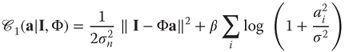

where corresponds to the steepness of the prior and to its scaling (see Figure 14.2 from Ref. [46]). This choice is often favored because it results in a convex cost for which known numerical optimization methods such as conjugate gradient may be used. In particular, these terms may be put in parallel to regularization terms that are used in computer vision. For instance, an L2-norm penalty term corresponds to Tikhonov regularization [47] or an L1-norm term corresponds to the Lasso method. See Chapter 4 for a review of possible parameterization of this norm, for instance by using nested norms. Classical implementation of sparse coding relies therefore on a parametric measure of sparseness.

Let us now derive another measure of sparseness. Indeed, a nonparametric form of sparseness cost may be defined by considering that neurons representing the vector are either active or inactive. In fact, the spiking nature of neural information demonstrates that the transition from an inactive to an active state is far more significant at the coding timescale than smooth changes of the firing rate. This is, for instance, perfectly illustrated by the binary nature of the neural code in the auditory cortex of rats [16]. Binary codes also emerge as optimal neural codes for rapid signal transmission [48, 49]. This is also relevant for neuromorphic systems which transmit discrete events (such as a network packet). With a binary event-based code, the cost is only incremented when a new neuron gets active, regardless of the analog value. Stating that an active neuron carries a bounded amount of information of bits, an upper bound for the representation cost of neural activity on the receiver end is proportional to the count of active neurons, that is, to the pseudo-norm :

14.4

This cost is similar to information criteria such as the Akaike information criteria [50] or distortion rate [[51], p. 571]. This simple nonparametric cost has the advantage of being dynamic: the number of active cells for one given signal grows in time with the number of spikes reaching the target population. But Eq. (14.4) defines a harder cost to optimize (in comparison to Eq. (14.3) for instance) because the hard pseudo-norm sparseness leads to a nonconvex optimization problem which is NP-complete with respect to the dimension of the dictionary [[51], p. 418].

14.2.2 Learning to Be Sparse: The SparseNet Algorithm

We have seen above that we may define different models for measuring sparseness depending on our prior assumption on the distribution of coefficients. Note first that, assuming that the statistics are stationary (more generally ergodic), then these measures of sparseness across a population should necessarily imply a lifetime sparseness for any neuron. Such a property is essential to extend results from electrophysiology. Indeed, it is easier to record a restricted number of cells than a full population (see, for instance, Ref. [4]). However, the main property in terms of efficiency is that the representation should be sparse at any given time, that is, in our setting, at the presentation of each novel image.

Now that we have defined sparseness, how could we use it to induce neural organization? Indeed, given a sparse coding strategy that optimizes any representation efficiency cost as defined above, we may derive an unsupervised learning model by optimizing the dictionary over natural scenes. On the one hand, the flexibility in the definition of the sparseness cost leads to a wide variety of proposed sparse codingsolutions (for a review, see Ref. [52]) such as numerical optimization [22], non-negative matrix factorization [53, 54], or matching pursuit [26, 27, 29, 31]. They are all derived from correlation-based inhibition as this is necessary to remove redundancies from the linear representation. This is consistent with the observation that lateral interactions are necessary for the formation of elongated receptive fields [8, 55].

On the other hand, these methods share the same GLM model (see Eq. (14.1)) and once the sparse coding algorithm is chosen, the learning scheme is similar. As a consequence, after every coding sweep, we increased the efficiency of the dictionary with respect to Eq. (14.2). This is achieved using the online gradient descent approach given the current sparse solution, :

14.5

where is the learning rate. Similar to Eq. (17) in Ref. [22] or to Eq. (2) in Ref. [31], the relation is a linear “Hebbian” rule [33] because it enhances the weight of neurons proportionally to the correlation between pre- and postsynaptic neurons. Note that there is no learning for nonactivated coefficients. The novelty of this formulation compared to other linear Hebbian learning rule such as Ref. [56] is to take advantage of the sparse representation, hence the name sparse Hebbian learning (SHL).

The class of SHL algorithms are unstable without homeostasis, that is, without a process that maintains the system in a certain equilibrium. In fact, starting with a random dictionary, the first filters to learn are more likely to correspond to salient features [26] and are therefore more likely to be selected again in subsequent learning steps. In SparseNet, the homeostatic gain control is implemented by adaptively tuning the norm of the filters. This method equalizes the variance of coefficients across neurons using a geometric stochastic learning rule. The underlying heuristic is that this introduces a bias in the choice of the active coefficients. In fact, if a neuron is not selected often, the geometric homeostasis will decrease the norm of the corresponding filter, and therefore—from Eq. (14.1) and the conjugate gradient optimization—this will increase the value of the associated scalar. Finally, as the prior functions defined in Eq. (14.3) are identical for all neurons, this will increase the relative probability that the neuron is selected with a higher relative value. The parameters of this homeostatic rule have a great importance for the convergence of the global algorithm. In Reference [29], we have derived a more general homeostasis mechanism derived from the optimization of the representation efficiency through histogram equalization which we will describe later (see Section 14.4.1).

14.2.3 Results: Efficiency of Different Learning Strategies

The different SHL algorithms simply differ in the coding step. This implies that they only differ by first how sparseness is defined at a functional level and second how the inverse problem corresponding to the coding step is solved at the algorithmic level. Most of the schemes cited above use a less strict, parametric definition of sparseness (such as the convex L-norm), but for which a mathematical formulation of the optimization problem exists. Few studies such as Refs [57, 58] use the stricter pseudo-norm as the coding problem gets more difficult. A thorough comparison of these different strategies was recently presented in Ref. [59]. See also Ref. [60] for properties of the coding solutions to the pseudo-norm. Similarly, in Ref. [29], we preferred to retrieve an approximate solution to the coding problem to have a better match with the measure of efficiency Eq. (14.4).

Such an algorithmic framework is implemented in the SHL-scripts package.² These scripts allow the retrieval of the database of natural images and the replication of the results of Ref. [29] reported in this section. With a correct tuning of parameters, we observed that different coding schemes show qualitatively a similar emergence of edge-like filters. The specific coding algorithm used to obtain this sparseness appears to be of secondary importance as long as it is adapted to the data and yields sufficiently efficient sparse representation vectors. However, resulting dictionaries vary qualitatively among these schemes and it was unclear which algorithm is the most efficient and what was the individual role of the different mechanisms that constitute SHL schemes. At the learning level, we have shown that the homeostasis mechanism had a great influence on the qualitative distribution of learned filters [29].

The results are shown in Figure 14.1. This figure represents the qualitative results of the formation of edge-like filters (receptive fields). More importantly, it shows the quantitative results as the average decrease of the squared error as a function of the sparseness. This gives a direct access to the cost as computed in Eq. (14.4). These results are comparable with the sparsenet algorithm. Moreover, this solution, by giving direct access to the atoms (filters) that are chosen, provides us with a more direct tool to manipulate sparse components. One further advantage consists in the fact that this unsupervised learning model is nonparametric (compare with Eq. (14.3)) and thus does not need to be parametrically tuned. Results show the role of homeostasis on the unsupervised algorithm. In particular, using the comparison of coding and decoding efficiency with and without this specific homeostasis, we have proven that cooperative homeostasis optimized overall representation efficiency (see also Section 14.4.1).

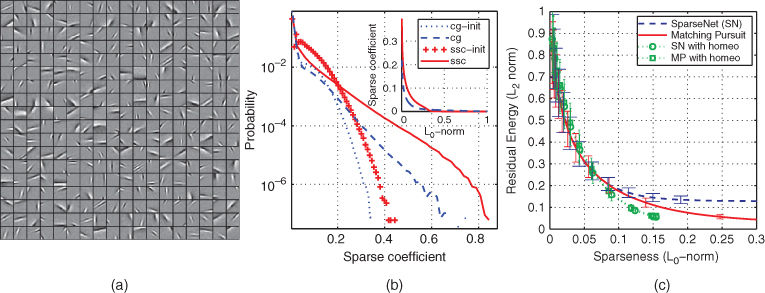
Figure 14.1 Learning a sparse code using sparse Hebbian learning. (a) We show the results at convergence (20,000 learning steps) of a sparse model with unsupervised learning algorithm which progressively optimizes the relative number of active (nonzero) coefficients ( pseudo-norm) [29]. Filters of the same size as the image patches are presented in a matrix (separated by a black border). Note that their position in the matrix is arbitrary as in ICA. These results show that sparseness induces the emergence of edge-like receptive fields similar to those observed in the primary visual area of primates. (b) We show the probability distribution function of sparse coefficients obtained by our method compared to Ref. [21] with first random dictionaries (respectively, “ssc-init” and “cg-init”) and second with the dictionaries obtained after convergence of respective learning schemes (respectively, “ssc” and “cg”). At convergence, sparse coefficients are more sparsely distributed than initially, with more kurtotic probability distribution functions for “ssc” in both cases, as can be seen in the “longer tails” of the distribution. (c) We evaluate the coding efficiency of both methods with or without cooperative homeostasis by plotting the average residual error (L norm) as a function of the pseudo-norm. This provides a measure of the coding efficiency for each dictionary over the set of image patches (error bars represent one standard deviation). The best results are those providing a lower error for a given sparsity (better compression) or a lower sparseness for the same error.

It is at this point important to note that in this algorithm, we achieve an exponential convergence of the squared error [[51], p. 422], but also that this curve can be directly derived from the coefficients' values. Indeed, for coefficients (i.e., ), we have the squared error equal to

14.6

As a consequence, the sparser the distributions of coefficients, the quicker is the decrease of the residual energy. In the following section, we describe different variations of this algorithm. To compare their respective efficiency, we plot the decrease of the coefficients along with the decrease of the residual's energy. Using such tools, we explore whether such a property extends to full-scale images and not only to image patches, an important condition for using sparse models in computer vision algorithms.

14.3 SparseLets: A Multiscale, Sparse, Biologically Inspired Representation of Natural Images

14.3.1 Motivation: Architecture of the Primary Visual Cortex

Our goal here is to build practical algorithms of sparse coding for computer vision. We have seen above that it is possible to build an adaptive model of sparse coding that we applied to image patches. Invariably, this has shown that the independent components of image patches are edge-like filters, such as are found in simple cells of V1. This model has shown that for randomly chosen image patches, these may be described by a sparse vector of coefficients. Extending this result to full-field natural images, we can expect that this sparseness would increase by a degree of order. In fact, except in a densely cluttered image such as a close-up of a texture, natural images tend to have wide areas which are void (such as the sky, walls, or uniformly filled areas). However, applying directly the sparsenet algorithm to full-field images is impossible in practice as its computer simulation would require too much memory to store the overcomplete set of filters. However, it is still possible to define a priori these filters and herein, we focus on a full-field sparse coding method whose filters are inspired by the architecture of the primary visual cortex.

The first step of our method involves defining the dictionary of templates (or filters) for detecting edges. We use a log-Gabor representation, which is well suited to represent a wide range of natural images [42]. This representation gives a generic model of edges parameterized by their shape, orientation, and scale. We set the range of these parameters to match with what has been reported for simple-cell responses in macaque primary visual cortex (V1). Indeed, log-Gabor filters are similar to standard Gabors and both are well fitted to V1 simple cells [61]. Log-Gabors are known to produce a sparse set of linear coefficients [62]. Similarly to Gabors, these filters are defined by Gaussians in Fourier space, but their specificity is that log-Gabors have Gaussians envelopes in log-polar frequency space. This is consistent with physiological measurements which indicate that V1 cell responses are symmetric on the log frequency scale. They have multiple advantages over Gaussians: in particular, they have no DC component, and more generally, their envelopes more broadly cover the frequency space [63]. In this chapter, we set the bandwidth of the Fourier representation of the filters to and , respectively in the log-frequency and polar coordinates to get a family of relatively elongated (and thus selective) filters (see Ref. [63] and Figure 14.2(a) for examples of such edges). Before to the analysis of each image, we used the spectral whitening filter described by Olshausen and Field [22] to provide a good balance of the energy of output coefficients [26, 42]. Such a representation is implemented in the LogGabor package.³

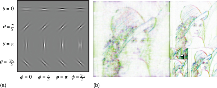
Figure 14.2 The log-Gabor pyramid (a) A set of log-Gabor filters showing in different rows different orientations and in different columns, different phases. Here we have only shown one scale. Note the similarity with Gabor filters. (b) Using this set of filters, one can define a linear representation that is rotation-, scaling- and translation-invariant. Here we show a tiling of the different scales according to a golden pyramid [43]. The hue gives the orientation while the value gives the absolute value (white denotes a low coefficient). Note the redundancy of the linear representation, for instance, at different scales.

This transform is linear and can be performed by a simple convolution repeated for every edge type. Following [63], convolutions were performed in the Fourier (frequency) domain for computational efficiency. The Fourier transform allows for a convenient definition of the edge filter characteristics, and convolution in the spatial domain is equivalent to a simple multiplication in the frequency domain. By multiplying the envelope of the filter and the Fourier transform of the image, one may obtain a filtered spectral image that may be converted to a filtered spatial image using the inverse Fourier transform. We exploited the fact that by omitting the symmetrical lobe of the envelope of the filter in the frequency domain, we obtain quadrature filters. Indeed, the output of this procedure gives a complex number whose real part corresponds to the response to the symmetrical part of the edge, while the imaginary part corresponds to the asymmetrical part of the edge (see Ref. [63] for more details). More generally, the modulus of this complex number gives the energy response to the edge—as can be compared to the response of complex cells in area V1, while its argument gives the exact phase of the filter (from symmetric to nonsymmetric). This property further expands the richness of the representation.

Given a filter at a given orientation and scale, a linear convolution model provides a translation-invariant representation. Such invariance can be extended to rotations and scalings by choosing to multiplex these sets of filters at different orientations and spatial scales. Ideally, the parameters of edges would vary in a continuous fashion to a full relative translation, rotation, and scale invariance. However this is difficult to achieve in practice and some compromise has to be found. Indeed, although orthogonal representations are popular in computer vision owing to their computational tractability, it is desirable in our context that we have a relatively high overcompleteness in the representation to achieve this invariance. For a given set of images, we first chose to have dyadic levels (i.e., by doubling the scale at each level) with different orientations. Orientations are measured as nonoriented angles in radians, by convention in the range from to (but not including ) with respect to the -axis. Finally, each image is transformed into a pyramid of coefficients. This pyramid consists of approximately pixels multiplexed on scales and orientations, that is, approximately coefficients, an overcompleteness factor of about . This linear transformation is represented by a pyramid of coefficients, see Figure 14.2(b).

14.3.2 The SparseLets Framework

The resulting dictionary of edge filters is overcomplete. The linear representation would thus give a dense, relatively inefficient representation of the distribution of edges, see Figure 14.2(b). Therefore, starting from this linear representation, we searched instead for the most sparse representation. As we saw above in Section 14.2, minimizing the pseudo-norm (the number of nonzero coefficients) leads to an expensive combinatorial search with regard to the dimension of the dictionary (it is NP-hard). As proposed by Perrinet [26], we may approximate a solution to this problem using a greedy approach. Such an approach is based on the physiology of V1. Indeed, it has been shown that inhibitory interneurons decorrelate excitatory cells to drive sparse code formation [55, 64]. We use this local architecture to iteratively modify the linear representation [42].

In general, a greedy approach is applied when the optimal combination is difficult to solve globally, but can be solved progressively, one element at a time. Applied to our problem, the greedy approach corresponds to first choosing the single filter that best fits the image along with a suitable coefficient , such that the single source is a good match to the image. Examining every filter , we find the filter with the maximal correlation coefficient (“matching” step), where

14.7

represents the inner product and represents the (Euclidean) norm. The index (“address”) gives the position ( and ), scale and orientation of the edge. We saw above that as filters at a given scale and orientation are generated by a translation, this operation can be efficiently computed using a convolution, but we keep this notation for its generality. The associated coefficient is the scalar projection

14.8

Second, knowing this choice, the image can be decomposed as

14.9

where is the residual image (“pursuit” step). We then repeat this two-step process on the residual (i.e., with ) until some stopping criterion is met. Note also that the norm of the filters has no influence in this algorithm on the matching step or on the reconstruction error. For simplicity and without loss of generality, we will hereafter set the norm of the filters to : (i.e., the spectral energy sums to 1). Globally, this procedure gives us a sequential algorithm for reconstructing the signal using the list of sources (filters with coefficients), which greedily optimizes the pseudo-norm (i.e., achieves a relatively sparse representation given the stopping criterion). The procedure is known as the matching pursuit (MP) algorithm [65], which has been shown to generate good approximations for natural images [26, 29].

We have included two minor improvements over this method: first, we took advantage of the response of the filters as complex numbers. As stated above, the modulus gives a response independent of the phase of the filter, and this value was used to estimate the best match of the residual image with the possible dictionary of filters (matching step). Then, the phase was extracted as the argument of the corresponding coefficient and used to feed back onto the image in the pursuit step. This modification allows for a phase-independent detection of edges, and therefore for a richer set of configurations, while preserving the precision of the representation.

Second, we used a “smooth” pursuit step. In the original form of the MP algorithm, the projection of the matching coefficient is fully removed from the image, which allows for the optimal decrease of the energy of the residual and allows for the quickest convergence of the algorithm with respect to the pseudo-norm (i.e., it rapidly achieves a sparse reconstruction with low error). However, this efficiency comes at a cost, because the algorithm may result in nonoptimal representations because of choosing edges sequentially and not globally. This is often a problem when edges are aligned (e.g., on a smooth contour), as the different parts will be removed independently, potentially leading to a residual with gaps in the line. Our goal here is not necessarily to get the fastest decrease of energy, but rather to provide with the best representation of edges along contours. We therefore used a more conservative approach, removing only a fraction (denoted by ) of the energy at each pursuit step (for MP, ). Note that in that case, Eq. (14.6) has to be modified to account for the parameter:

14.10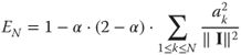

We found that was a good compromise between rapidity and smoothness. One consequence of using is that, when removing energy along contours, edges can overlap; even so, the correlation is invariably reduced. Higher and smaller values of were also tested, and gave representation results similar to those presented here.

In summary, the whole coding algorithm is given by the following nested loops in pseudo-code:

1. draw a signal from the database; its energy is ,

2. initialize sparse vector to zero and linear coefficients ,

3. while the residual energy is above a given threshold do:

a. select the best match: , where denotes the modulus,

b. increment the sparse coefficient: ,

c. update residual image: ,

d. update residual coefficients: ,

4. the final set of nonzero values of the sparse representation vector constitutes the list of edges representing the image as the list of couples , where represents an edge occurrence as represented by its position, orientation and scale and the complex-valued sparse coefficient.

This class of algorithms gives a generic and efficient representation of edges, as illustrated by the example in Figure 14.3(a). We also verified that the dictionary used here is better adapted to the extraction of edges than Gabor's [42]. The performance of the algorithm can be measured quantitatively by reconstructing the image from the list of extracted edges. All simulations were performed using Python (version 2.7.8) with packages NumPy (version 1.8.1) and SciPy (version 0.14.0) [66] on a cluster of Linux computing nodes. Visualization was performed using Matplotlib (version 1.3.1) [67].⁴

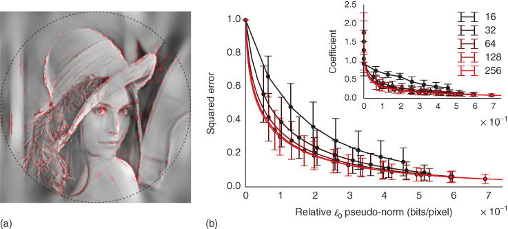
Figure 14.3 SparseLets framework. (a) An example reconstructed image with the list of extracted edges overlaid. As in Ref. [68], edges outside the circle are discarded to avoid artifacts. Parameters for each edge are the position, orientation, scale (length of bar), and scalar amplitude (transparency) with the phase (hue). We controlled the quality of the reconstruction from the edge information such that the residual energy is less than over the whole set of images, a criterion met on average when identifying edges per image for images of size (i.e., a relative sparseness of of activated coefficients). (b) Efficiency for different image sizes as measured by the decrease of the residual's energy as a function of the coding cost (relative pseudo-norm). (b, inset) This shows that as the size of images increases, sparseness increases, validating quantitatively our intuition on the sparse positioning of objects in natural images. Note, that the improvement is not significant for a size superior to . The SparseLets framework thus shows that sparse models can be extended to full-scale natural images, and that increasing the size improves sparse models by a degree of order (compare a size of with that of ).

14.3.3 Efficiency of the SparseLets Framework

Figure 14.3(a), shows the list of edges extracted on a sample image. It fits qualitatively well with a rough sketch of the image. To evaluate the algorithm quantitatively, we measured the ratio of extracted energy in the images as a function of the number of edges on a database of 600 natural images of size ,⁵ see Figure 14.3(b). Measuring the ratio of extracted energy in the images, edges were enough to extract an average of approximately of the energy of images in the database. To compare the strength of the sparseness in these full-scale images compared to the image patches discussed above (see Section 14.2), we measured the sparseness values obtained in images of different sizes. For these to be comparable, we measured the efficiency with respect to the relative pseudo-norm in bits per unit of image surface (pixel): this is defined as the ratio of active coefficients times the numbers of bits required to code for each coefficient (i.e., , where is the total number of coefficients in the representation) over the size of the image. For different image and framework sizes, the lower this ratio, the higher the sparseness. As shown in Figure 14.3(b), we indeed see that sparseness increases relative to an increase in image size. This reflects the fact that sparseness is not only local (few edges coexist at one place) but is also spatial (edges are clustered, and most regions are empty). Such a behavior is also observed in V1 of monkeys as the size of the stimulation is increased from a stimulation over only the classical receptive field to 4 times around it [15].

Note that by definition, our representation of edges is invariant to translations, scalings, and rotations in the plane of the image. We also performed the same edge extraction where images from the database were perturbed by adding independent Gaussian noise to each pixel such that signal-to-noise ratio was halved. Qualitative results are degraded but qualitatively similar. In particular, edge extraction in the presence of noise may result in false positives. Quantitatively, one observes that the representation is slightly less sparse. This confirms our intuition that sparseness is causally linked to the efficient extraction of edges in the image.

To examine the robustness of the framework and of sparse models in general, we examined how results changed on changing the parameters for the algorithm. In particular, we investigated the effect of filter parameters and . We also investigated how the overcompleteness factor could influence the result. We manipulated the number of discretization steps along the spatial frequency axis (i.e., the number of layers in the pyramid) and orientation axis . The results are summarized in Figure 14.4 and show that an optimal efficiency is achieved for certain values of these parameters. These optimal values are in the order of that found for the range of selectivities observed in V1. Note that these values may change across categories. Further experiments should provide an adaptation mechanism to allow finding the best parameters in an unsupervised manner.

Figure 14.4 Effect of filters' parameters on the efficiency of the SparseLets framework. As we tested different parameters for the filters, we measured the gain in efficiency for the algorithm as the ratio of the code length to achieve 85% of energy extraction relative to that for the default parameters (white bar). The average is computed on the same database of natural images and error bars denote the standard deviation of gain over the database. First, we studied the effect of the bandwidth of filters respectively in the (a) spatial frequency and (b) orientation spaces. The minimum is reached for the default parameters: this shows that default parameters provide an optimal compromise between the precision of filters in the frequency and position domains for this database. We may also compare pyramids with different number of filters. Indeed from Eq. (14.4), efficiency (in bits) is equal to the number of selected filters times the coding cost for the address of each edge in the pyramid. We plot here the average gain in efficiency which shows an optimal compromise respectively (c) the number of orientations and (d) the number of spatial frequencies (scales). Note first that with more than 12 directions, the gain remains stable. Note also that a dyadic scale ratio (that is, of 2) is efficient but that other solutions—such as using the golden section —prove to be significantly more efficient, although the average gain is relatively small (inferior to 5%).

These particular results illustrate the potential of sparse models in computer vision. Indeed, one main advantage of these methods is to explicitly represent edges. A direct application of sparse models is the ability of the representation to reconstruct these images and therefore to use it for compression [26]. Other possible applications are image filtering or edge manipulation for texture synthesis or denoising [69]. Recent advances have shown that such representations could be used for the classification of natural images (see Chapter 13 or, for instance, Ref. [70]) or of medical images of emphysema [71]. Classification was also used in a sparse model for the quantification of artistic style through sparse coding analysis in the drawings of Pieter Bruegel the Elder [72]. These examples illustrate the different applications of sparse representations and in the following we illustrate some potential perspectives to further improve their representation efficiency.

14.4 SparseEdges: Introducing Prior Information

14.4.1 Using the Prior in First-Order Statistics of Edges

In natural images, it has been observed that edges follow some statistical regularities that may be used by the visual system. We first focus on the most obvious regularity which consists in the anisotropic distribution of orientations in natural images (see Chapter 4 for another qualitative characterization of this anisotropy). Indeed, it has been observed that orientations corresponding to cardinals (i.e., to verticals and horizontals) are more likely than other orientations [73, 74]. This is due to the fact that our point of view is most likely pointing toward the horizon while we stand upright. In addition, gravity shaped our surrounding world around horizontals (mainly the ground) and verticals (such as trees or buildings). Psychophysically, this prior knowledge gives rise to the oblique effect [75]. This is even more striking in images of human scenes (such as a street, or inside a building) as humans mainly build their environment (houses, furnitures) around these cardinal axes. However, we assumed in the cost defined above (see Eq. (14.2)) that each coefficient is independently distributed.

It is believed that a homeostasis mechanism allows one to optimize this cost knowing this prior information [29, 76]. Basically, the solution is to put more filters where there are more orientations [73] such that coefficients are uniformly distributed. In fact, as neural activity in the assembly actually represents the sparse coefficients, we may understand the role of homeostasis as maximizing the average representation cost . This is equivalent to saying that homeostasis should act such that at any time, and invariantly to the selectivity of features in the dictionary, the probability of selecting one feature is uniform across the dictionary. This optimal uniformity may be achieved in all generality by using an equalization of the histogram [7]. This method may be easily derived if we know the probability distribution function of variable (see Figure 14.5(a)) by choosing a nonlinearity as the cumulative distribution function (see Figure 14.5(b)) transforming any observed variable into

14.11

This is equivalent to the change of variables which transforms the sparse vector to a variable with uniform probability distribution function in (see Figure 14.5(c)). This equalization process has been observed in the neural activity of a variety of species and is, for instance, perfectly illustrated in the compound eye of the fly's neural response to different levels of contrast [76]. It may evolve dynamically to slowly adapt to varying changes, for instance to luminance or contrast values, such as when the light diminishes at twilight. Then, we use these point nonlinearities to sample orientation space in an optimal fashion (see Figure 14.5(d)).

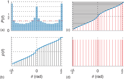
Figure 14.5 Histogram equalization. From the edges extracted in the images from the natural scenes database, we computed sequentially (clockwise, from the bottom left): (a) the histogram and (b) cumulative histogram of edge orientations. This shows that as was reported previously (see, for instance, Ref. [74]), cardinals axis are overrepresented. This represents a relative inefficiency as the representation in the SparseLets framework represents a priori orientations in a uniform manner. A neuromorphic solution is to use histogram equalization, as was first shown in the fly's compound eye by Laughlin [76]. (c) We draw a uniform set of scores on the -axis of the cumulative function (black horizontal lines), for which we select the corresponding orientations (red vertical lines). Note that by convention these are wrapped up to fit in the range. (d) This new set of orientations is defined such that they are a priori selected uniformly. Such transformation was found to well describe a range of psychological observations [73] and we will now apply it to our framework.

This simple nonparametric homeostatic method is applicable to the SparseLets algorithm by simply using the transformed sampling of the orientation space. It is important to note that the MP algorithm is nonlinear and the choice of one element at any step may influence the rest of the choices. In particular, while orientations around cardinals are more prevalent in natural images (see Figure 14.6(a)), the output histogram of detected edges is uniform (see Figure 14.6(b)). To quantify the gain in efficiency, we measured the residual energy in the SparseLets framework with or without including this prior knowledge. Results show that for a similar number of extracted edges, residual energy is not significantly changed (see Figure 14.6(c)). This is again due to the exponential convergence of the squared error [[51], p. 422] on the space spanned by the representation basis. As the tiling of the Fourier space by the set of filters is complete, one is assured of the convergence of the representation in both cases. However thanks to the use of first-order statistics, the orientation of edges are distributed such as to maximize the entropy, further improving the efficiency of the representation.

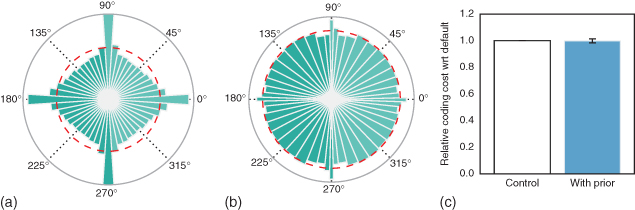
Figure 14.6 Including prior knowledge on the orientation of edges in natural images. (a) Statistics of orientations in the database of natural images as shown by a polar bar histogram (the surface of wedges is proportional to occurrences). As for Figure 14.5(a), this shows that orientations around cardinals are more likely than others (the dotted red line shows the average occurrence rate). (b) We show the histogram with the new set of orientations that has been used. Each bin is selected approximately uniformly. Note the variable width of bins. (c) We compare the efficiency of the modified algorithm where the sampling is optimized thanks to histogram equalization described in Figure 14.5 as the average residual energy with respect to the number of edges. This shows that introducing a prior information on the distribution of orientations in the algorithm may also introduce a slight but insignificant improvement in the sparseness.

This novel improvement to the SparseLets algorithm illustrates the flexibility of the MP framework. This proves that by introducing the prior on first-order statistics, one improves the efficiency of the model for this class of natural images. Of course, this gain is only valid for natural images and would disappear for images where cardinals would not dominate. This is the case for images of close-ups (microscopy) or where gravity is not prevalent such as aerial views. Moreover, this is obviously just a first step as there is more information from natural images that could be taken into account.

14.4.2 Using the Prior Statistics of Edge Co-Occurrences

A natural extension of the previous result is to study the co-occurrences of edges in natural images. Indeed, images are not simply built from independent edges at arbitrary positions and orientations but tend to be organized along smooth contours that follow, for instance, the shape of objects. In particular, it has been shown that contours are more likely to be organized along co-circular shapes [77]. This reflects the fact that in nature, round objects are more likely to appear than random shapes. Such a statistical property of images seems to be used by the visual system as it is observed that edge information is integrated on a local “association field” favoring colinear or co-circular edges (see Chapter 13, Section 5, for more details and a mathematical description). In V1 for instance, neurons coding for neighboring positions are organized in a similar fashion. We have previously seen that statistically, neurons coding for collinear edges seem to be anatomically connected [12, 13] while rare events (such as perpendicular occurrences) are functionally inhibited [13].

Using the probabilistic formulation of the edge extraction process (see Section 14.2), one can also apply this prior probability to the choice of mechanism (matching) of the MP algorithm. Indeed at any step of the edge extraction process, one can include the knowledge gained by the extraction of previous edges, that is, the set of extracted edges, to refine the log-likelihood of a new possible edge (where corresponds to the address of the chosen filter, and therefore to its position, orientation, and scale). Knowing the probability of co-occurrences from the statistics observed in natural images (see Figure 14.7), we deduce that the cost is now at any coding step (where is the residual image—see Eq. (14.9)):

14.12

where quantifies the strength of this prediction. Basically, this shows that, similarly to the association field proposed by Grossberg [78] which was subsequently observed in cortical neurons [79] and applied by Field et al. [80], we facilitate the activity of edges knowing the list of edges that were already extracted. This comes as a complementary local interaction to the inhibitory local interaction implemented in the pursuit step (see Eq. (14.9)) and provides a quantitative algorithm to the heuristics proposed in Ref. [42]. Note that although this model is purely sequential and feed-forward, this results possibly in a “chain rule” as when edges along a contour are extracted, this activity is facilitated along it as long as the image of this contour exists in the residual image. Such a “chain rule” is similar to what was used to model psychophysical performance [68] or to filter curves in images [81]. Our novel implementation provides a rapid and efficient solution that we illustrate here on a segmentation problem (see Figure 14.8).

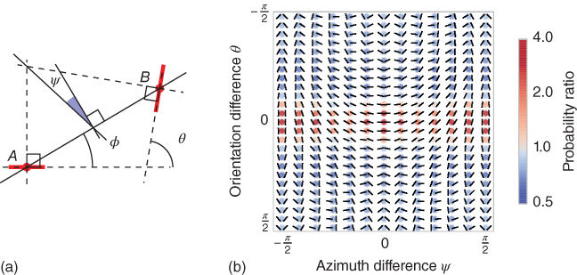
Figure 14.7 Statistics of edge co-occurrences. (a) The relationship between a pair of edges can be quantified in terms of the difference between their orientations , the ratio of scale relative to the reference edge, the distance between their centers, and the difference of azimuth (angular location) of the second edge relative to the reference edge. In addition, we define as it is symmetric with respect to the choice of the reference edge, in particular, for co-circular edges. (b) The probability distribution function represents the distribution of the different geometrical arrangements of edges' angles, which we call a “chevron map.” We show here the histogram for natural images, illustrating the preference for colinear edge configurations. For each chevron configuration, deeper and deeper red circles indicate configurations that are more and more likely with respect to a uniform prior, with an average maximum of about times more likely, and deeper and deeper blue circles indicate configurations less likely than a flat prior (with a minimum of about times as likely). Conveniently, this “chevron map” shows in one graph that natural images have on average a preference for colinear and parallel angles (the horizontal middle axis), along with a slight preference for co-circular configurations (middle vertical axis).

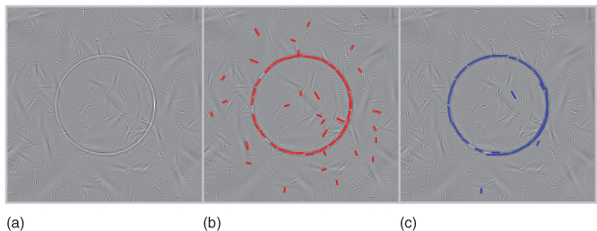
Figure 14.8 Application to rapid contour segmentation. We applied the original sparse edge framework to (a) the synthetic image of a circle embedded in noise. This noise is synthesized by edges at random positions, orientations and scales with a similar first-order statistics as natural scenes. (b) We overlay in red the set of edges which were detected by the SparseLets framework. (c) Then, we introduce second-order information in the evaluation of the probability in the sparse edges framework (with ). This modifies the sequence of extracted edges as shown in blue. There is a clear match of the edge extraction with the circle, as would be predicted by psychophysical results of hand segmentation of contours. This shows that second-order information as introduced in this feed-forward chain may be sufficient to account for contour grouping and may not necessitate a recursive chain rule such as implemented in Ref. [68].

Indeed, sparse models have been shown to foster numerous applications in computer vision. Among these are algorithms for segmentation in images [82] or for classification [83, 84]. We may use the previous application of our algorithm to evaluate the probability of edges belonging to the same contour. We show in Figure 14.8 the application of such a formula (in panel c vs classical sparse edge extraction in panel b) on a synthetic image of a circle embedded in noise (panel a). It shows that, while some edges from the background are extracted in the plain SparseLets framework (panel b), edges belonging to the same circular contour pop out from the computation similar to a chain rule (panel c). Note that contrary to classical hierarchical models, these results have been obtained with a simple layer of edge detection filters which communicate through local diffusion. An important novelty to note in this extension of the SparseLets framework is that there is no recursive propagation, as the greedy algorithm is applied in a sequential manner. These types of interaction have been found in area V1. Indeed, the processing may be modulated by simple contextual rules such as favoring colinear versus co-circular edges [85]. Such type of modulation opens up a wide range of potential applications to computer vision such as robust segmentation and algorithms for the autonomous classification of images [70]. More generally, it shows that simple feed-forward algorithms such as the one we propose may be sufficient to account for the sparse representation of images in lower-level visual areas.

14.5 Conclusion

In this chapter, we have shown sparse models at increasing structural complexities mimicking the key features of the primary visual cortex in primates. By focusing on a concrete example, the SparseLets framework, we have shown that sparse models provide an efficient framework for biologically inspired computer vision algorithms. In particular, by including contextual information, such as prior statistics on natural images, we could improve the efficiency of the sparseness of the representation.

Such an approach allows to implement a range of practical concepts (such as the good continuity of contours) in a principled way. Indeed, we based our reasoning on inferential processes such as they are reflected in the organization of neural structures. For instance, there is a link between co-circularity and the structure of orientation maps [86]. This should be included in further perspectives of these sparse models.

As we have seen, the (visual) brain is not a computer. Instead of using a sequential stream of semantic symbols, it uses statistical regularities to derive predictive rules. These computations are not written explicitly as it suffices that they emerge from the collective behavior in populations of neurons. As such, these rules are massively parallel, asynchronous, and error prone. Luckily, such neuromorphic computing architectures are beginning to emerge—yet, we lack a better understanding of how we may implement computer vision algorithms on such hardware.

In conclusion, this drives the need for a more biologically driven computer vision algorithm and a better understanding of V1. However, such knowledge is largely incomplete [87] and we need to develop a better understanding of results from electrophysiology. A promising approach in that sense is to include model-driven stimulation of physiological studies [88, 89] as they systematically test neural computations for a given visual task.

Acknowledgments

The author was supported by EC IP project FP7-269921, “BrainScaleS”. Correspondence and requests for materials should be addressed to the author (email:Laurent.Perrinet@univ-amu.fr).

References

1. 1. Friston, K., Adams, R.A., Perrinet, L., and Breakspear, M. (2012) Perceptions as hypotheses: saccades as experiments. Front. Psychol., 3, doi: 10.3389/fpsyg.2012.00151

2. 2. Hubel, D. and Wiesel, T. (1968) Receptive fields and functional architecture of monkey's striate cortex. J. Physiol., 195 (1), 215–244, http://www.ncbi.nlm.nih.gov/pmc/articles/PMC1557912/.

3. 3. Barth, A.L. and Poulet, J.F.A. (2012) Experimental evidence for sparse firing in the neocortex. Trends Neurosci., 35 (6), 345–355, doi: 10.1016/j.tins.2012.03.008

4. 4. Willmore, B.D., Mazer, J.A., and Gallant, J.L. (2011) Sparse coding in striate and extrastriate visual cortex. J. Neurophysiol., 105 (6), 2907–2919, doi: 10.1152/jn.00594.2010

5. 5. Marr, D. (1983) Vision: A Computational Investigation into the Human Representation and Processing of Visual Information, Henry Holt and Company, Inc., http://www.worldcat.org/isbn/0716715678.

6. 6. Attneave, F. (1954) Some informational aspects of visual perception. Psychol. Rev., 61 (3), 183–193, http://view.ncbi.nlm.nih.gov/pubmed/13167245.

7. 7. Atick, J.J. (1992) Could information theory provide an ecological theory of sensory processing? Netw. Comput. Neural Syst., 3 (2), 213–252.

8. 8. Wolfe, J., Houweling, A.R., and Brecht, M. (2010) Sparse and powerful cortical spikes. Curr. Opin. Neurobiol., 20 (3), 306–312, doi: 10.1016/j.conb.2010.03.006

9. 9. Field, D.J. (1994) What is the goal of sensory coding? Neural Comput., 6 (4), 559–601, doi: 10.1162/neco.1994.6.4.559

10.10. Froudarakis, E., Berens, P., Ecker, A.S., Cotton, R.J., Sinz, F.H., Yatsenko, D., Saggau, P., Bethge, M., and Tolias, A.S. (2014) Population code in mouse V1 facilitates readout of natural scenes through increased sparseness. Nat. Neurosci., 17 (6), 851–857, doi: 10.1038/nn.3707

11.11. Palm, G. (2013) Neural associative memories and sparse coding. Neural Netw., 37, 165–171, doi: 10.1016/j.neunet.2012.08.013

12.12. Bosking, W.H., Zhang, Y., Schofield, B., and Fitzpatrick, D. (1997) Orientation selectivity and the arrangement of horizontal connections in tree shrew striate cortex. J. Neurosci., 17 (6), 2112–2127, http://www.jneurosci.org/cgi/content/abstract/17/6/2112.

13.13. Hunt, J.J., Bosking, W.H., and Goodhill, G.J. (2011) Statistical structure of lateral connections in the primary visual cortex. Neural Syst. Circ., 1 (1), 3, doi: 10.1186/2042-1001-1-3

14.14. Field, D.J. (1987) Relations between the statistics of natural images and the response properties of cortical cells. J. Opt. Soc. Am. A, 4 (12), 2379–2394.

15.15. Vinje, W.E. and Gallant, J.L. (2000) Sparse coding and decorrelation in primary visual cortex during natural vision. Science, 287 (5456), 1273–1276, doi: 10.1126/science.287.5456.1273

16.16. DeWeese, M.R., Wehr, M., and Zador, A.M. (2003) Binary spiking in auditory cortex. J. Neurosci., 23 (21), 7940–7949, http://www.jneurosci.org/content/23/21/7940.abstract.

17.17. Baudot, P., Levy, M., Marre, O., Monier, C., Pananceau, M., and Frégnac, Y. (2013) Animation of natural scene by virtual eye-movements evokes high precision and low noise in V1 neurons. Front. Neural Circ., 7, doi: 10.3389/fncir.2013.00206

18.18. Rao, R.P.N. and Ballard, D.H. (1999) Predictive coding in the visual cortex: a functional interpretation of some extra-classical receptive-field effects. Nat. Neurosci., 2 (1), 79–87, doi: 10.1038/4580

19.19. Spratling, M.W. (2011) A single functional model accounts for the distinct properties of suppression in cortical area V1. Vision Res., 51 (6), 563–576, doi: 10.1016/j.visres.2011.01.017

20.20. Perrinet, L.U., Adams, R.A., and Friston, K.J. (2014) Active inference, eye movements and oculomotor delays. Biol. Cybern., pp. 1–25, doi: 10.1007/s00422-014-0620-8

21.21. Olshausen, B.A. and Field, D.J. (1996) Natural image statistics and efficient coding. Netw. Comput. Neural Syst., 7 (6583), 333–339, doi: 10.1038/381607a0

22.22. Olshausen, B.A. and Field, D.J. (1997) Sparse coding with an overcomplete basis set: a strategy employed by V1? Vision Res., 37 (23), 3311–3325, doi: 10.1016/S0042-6989(97)00169-7

23.23. Bell, A.J. and Sejnowski, T.J. (1997) The ‘independent components’ of natural scenes are edge filters. Vision Res., 37 (23), 3327–3338.

24.24. Fyfe, C. and Baddeley, R. (1995) Finding compact and sparse-distributed representations of visual images. Netw. Comput. Neural Syst., 6 (3), 333–344, doi: 10.1088/0954-898X/6/3/002

25.25. Zibulevsky, M. and Pearlmutter, B.A. (2001) Blind source separation by sparse decomposition. Neural Comput., 13 (4), 863–882.

26.26. Perrinet, L., Samuelides, M., and Thorpe, S. (2004) Coding static natural images using spiking event times: do neurons cooperate? IEEE Trans. Neural Netw., 15 (5), 1164–1175, doi: 10.1109/TNN.2004.833303, special issue on 'Temporal Coding for Neural Information Processing'

27.27. Rehn, M. and Sommer, F.T. (2007) A model that uses few active neurons to code visual input predicts the diverse shapes of cortical receptive fields. J. Comput. Neurosci., 22 (2), 135–146.

28.28. Doi, E., Balcan, D.C., and Lewicki, M.S. (2007) Robust coding over noisy overcomplete channels. IEEE Trans. Image Process., 16 (2), 442–452.

29.29. Perrinet, L.U. (2010) Role of homeostasis in learning sparse representations. Neural Comput., 22 (7), 1812–1836, doi: 10.1162/neco.2010.05-08-795, http://invibe.net/LaurentPerrinet/Publications/Perrinet10shl.

30.30. Lewicki, M.S. and Sejnowski, T.J. (2000) Learning overcomplete representations. Neural Comput., 12 (2), 337–365.

31.31. Smith, E.C. and Lewicki, M.S. (2006) Efficient auditory coding. Nature, 439 (7079), 978–982, doi: 10.1038/nature04485

32.32. Baddeley, R., Abbott, L.F., Booth, M.C.A., Sengpiel, F., Freeman, T., Wakeman, E.A., and Rolls, E.T. (1997) Responses of neurons in primary and inferior temporal visual cortices to natural scenes. Proc. R. Soc. B: Biol. Sci., 264 (1389), 1775–1783, doi: 10.1098/rspb.1997.0246, http://citeseer.nj.nec.com/19262.html

33.33. Hebb, D.O. (1949) The Organization of Behavior: A Neuropsychological Theory, John Wiley & Sons, Inc., New York.

34.34. Zylberberg, J., Murphy, J.T., and DeWeese, M.R. (2011) A sparse coding model with synaptically local plasticity and spiking neurons can account for the diverse shapes of V1 simple cell receptive fields. PLoS Comput. Biol., 7 (10), e1002 250, doi: 10.1371/journal.pcbi.1002250

35.35. Hunt, J.J., Dayan, P., and Goodhill, G.J. (2013) Sparse coding can predict primary visual cortex receptive field changes induced by abnormal visual input. PLoS Comput. Biol., 9 (5), e1003 005, doi: 10.1371/journal.pcbi.1003005

36.36. Blättler, F. and Hahnloser, R.H.R. (2011) An efficient coding hypothesis links sparsity and selectivity of neural responses. PLoS ONE, 6 (10), e25 506, doi: 10.1371/journal.pone.0025506

37.37. Seriès, P., Latham, P.E., and Pouget, A. (2004) Tuning curve sharpening for orientation selectivity: coding efficiency and the impact of correlations. Nat. Neurosci., 7 (10), 1129–1135, doi: 10.1038/nn1321

38.38. Ganguli, S. and Sompolinsky, H. (2012) Compressed sensing, sparsity, and dimensionality in neuronal information processing and data analysis. Annu. Rev. Neurosci., 35 (1), 485–508, doi: 10.1146/annurev-neuro-062111-150410, http://keck.ucsf.edu/surya/12.CompSense.pdf.

39.39. Elad, M. (2010) Sparse and Redundant Representations: From Theory to Applications in Signal and Image Processing, 1st edn, Springer-Verlag, http://www.amazon.com/exec/obidos/redirect?tag=citeulike07-20&path=ASIN/144197010X.

40.40. Benoit, A., Caplier, A., Durette, B., and Herault, J. (2010) Using human visual system modeling for bio-inspired low level image processing. Comput. Vis. Image Underst., 114 (7), 758–773, doi: 10.1016/j.cviu.2010.01.011

41.41. Serre, T. and Poggio, T. (2010) A neuromorphic approach to computer vision. Commun. ACM, 53 (10), 54–61, doi: 10.1145/1831407.1831425

42.42. Fischer, S., Redondo, R., Perrinet, L.U., and Cristóbal, G. (2007) Sparse approximation of images inspired from the functional architecture of the primary visual areas. EURASIP J. Adv. Signal Process., 2007 (1), 090 727–090 122, doi: 10.1155/2007/90727

43.43. Perrinet, L.U. (2008) Adaptive sparse spike coding: applications of neuroscience to the compression of natural images, in Optical and Digital Image Processing Conference 7000 - Proceedings of SPIE, 7 - 11 April 2008, vol. 7000 (ed. G.C. Peter Schelkens), SPIE.

44.44. Perrinet, L.U. (2007) Topics in dynamical neural networks: from large scale neural networks to motor control and vision, in The European Physical Journal (Special Topics), vol. 142, Springer-Verlag, Berlin and Heidelberg, pp. 163–225, doi: 10.1016/j.jphysparis.2007.10.011

45.45. Rissanen, J. (1978) Modeling by shortest data description. Automatica, 14, 465–471.

46.46. Olshausen, B.A. (2002) Sparse codes and spikes, in Probabilistic Models of the Brain: Perception and Neural Function (eds R.P.N. Rao, B.A. Olshausen, and M.S. Lewicki), MIT Press, pp. 257–272.

47.47. Tikhonov, A.N. (1977) Solutions of Ill-Posed Problems, Winston & Sons, Washington, DC, http://www.amazon.com/exec/obidos/redirect?tag=citeulike07-20&path=ASIN/0470991240.

48.48. Bethge, M., Rotermund, D., and Pawelzik, K. (2003) Second order phase transition in neural rate coding: binary encoding is optimal for rapid signal transmission. Phys. Rev. Lett., 90 (8), 088 104.

49.49. Nikitin, A.P., Stocks, N.G., Morse, R.P., and McDonnell, M.D. (2009) Neural population coding is optimized by discrete tuning curves. Phys. Rev. Lett., 103 (13), 138 101.

50.50. Akaike, H. (1974) A new look at the statistical model identification. IEEE Trans. Autom. Control, 19, 716–723.

51.51. Mallat, S. (1998) A Wavelet Tour of Signal Processing, 2nd edn, Academic Press.

52.52. Pece, A.E.C. (2002) The problem of sparse image coding. J. Math. Imaging Vis., 17, 89–108.

53.53. Lee, D.D. and Seung, S.H. (1999) Learning the parts of objects by non-negative matrix factorization. Nature, 401, 788–791.

54.54. Ranzato, M.A., Poultney, C.S., Chopra, S., and LeCun, Y. (2007) Efficient learning of sparse overcomplete representations with an Energy-Based model. Adv. Neural Inf. Process. Syst., 19, 1137–1144.

55.55. Bolz, J. and Gilbert, C.D. (1989) The role of horizontal connections in generating long receptive fields in the cat visual cortex. Eur. J. Neurosci., 1 (3), 263–268.

56.56. Oja, E. (1982) A simplified neuron model as a principal component analyzer. J. Math. Biol., 15, 267–273.

57.57. Liu, J. and Jia, Y. (2014) Hebbian-based mean shift for learning the diverse shapes of V1 simple cell receptive fields. Chin. Sci. Bull., 59 (4), 452–458, doi: 10.1007/s11434-013-0041-4

58.58. Peharz, R. and Pernkopf, F. (2012) Sparse nonnegative matrix factorization with l0-constraints. Neurocomputing, 80, 38–46, doi: 10.1016/j.neucom.2011.09.024

59.59. Charles, A.S., Garrigues, P., and Rozell, C.J. (2012) A common network architecture efficiently implements a variety of Sparsity-Based inference problems. Neural Comput., 24 (12), 3317–3339, doi: 10.1162/neco_a_00372, http://citeseerx.ist.psu.edu/viewdoc/download?doi=10.1.1.310.2639&rep=rep1&type=pdf.

60.60. Aharon, M., Elad, M., and Bruckstein, A.M. (2006) On the uniqueness of overcomplete dictionaries, and a practical way to retrieve them. Linear Algebra Appl., 416 (1), 48–67, doi: 10.1016/j.laa.2005.06.035

61.61. Daugman, J.G. (1980) Two-dimensional spectral analysis of cortical receptive field profiles. Vision Res., 20 (10), 847–856, doi: 10.1016/0042-6989(80)90065-6

62.62. Field, D.J. (1999) Wavelets, vision and the statistics of natural scenes. Philos. Trans. R. Soc. London, Ser. A, 357 (1760), 2527–2542, doi: 10.1098/rsta.1999.0446

63.63. Fischer, S., Sroubek, F., Perrinet, L.U., Redondo, R., and Cristóbal, G. (2007) Self-invertible 2D log-Gabor wavelets. Int. J. Comput. Vision, 75 (2), 231–246, doi: 10.1007/s11263-006-0026-8

64.64. King, P.D., Zylberberg, J., and DeWeese, M.R. (2013) Inhibitory interneurons decorrelate excitatory cells to drive sparse code formation in a spiking model of V1. J. Neurosci., 33 (13), 5475–5485, doi: 10.1523/jneurosci.4188-12.2013

65.65. Mallat, S. and Zhang, Z. (1993) Matching Pursuit with time-frequency dictionaries. IEEE Trans. Signal Process., 41 (12), 3397–3414.

66.66. Oliphant, T.E. (2007) Python for scientific computing. Comput. Sci. Eng., 9 (3), 10–20, doi: 10.1109/MCSE.2007.58

67.67. Hunter, J.D. (2007) Matplotlib: a 2D graphics environment. Comput. Sci. Eng., 9 (3), 90–95, doi: 10.1109/MCSE.2007.55

68.68. Geisler, W.S., Perry, J.S., Super, B.J., and Gallogly, D.P. (2001) Edge co-occurence in natural images predicts contour grouping performance. Vision Res., 41 (6), 711–724, doi: 10.1016/s0042-6989(00)00277-7

69.69. Portilla, J. and Simoncelli, E.P. (2000) A parametric texture model based on joint statistics of complex wavelet coefficients. Int. J. Comput. Vision, 40 (1), 49–70, doi: 10.1023/a:1026553619983

70.70. Perrinet, L.U. and Bednar, J.A. (2014) Edge co-occurrences are sufficient to categorize natural versus animal images. Scientific Reports (2015), doi: 10.1038/srep11400.

71.71. Nava, R., Marcos, J.V., Escalante-Ramírez, B., Cristóbal, G., Perrinet, L.U., and Estépar, R.S.J. (2013) Advances in Texture Analysis for Emphysema Classification, Lecture Notes in Computer Science, vol. 8259, Chapter 27, Springer-Verlag, Berlin and Heidelberg, pp. 214–221, doi: 10.1007/978-3-642-41827-3_27

72.72. Hughes, J.M., Graham, D.J., and Rockmore, D.N. (2010) Quantification of artistic style through sparse coding analysis in the drawings of Pieter Bruegel the Elder. Proc. Natl. Acad. Sci., 107 (4), 1279–1283, doi: 10.1073/pnas.0910530107

73.73. Ganguli, D. and Simoncelli, E. (2010) Implicit encoding of prior probabilities in optimal neural populations, in Advances in Neural Information Processing Systems, vol. 23 (eds J. Lafferty, C.K.I. Williams, J. Shawe-Taylor, R.S. Zemel, and A. Culotta), pp. 658–666, http://www.cns.nyu.edu/pub/lcv/ganguli10c-preprint.pdf.

74.74. Girshick, A.R., Landy, M.S., and Simoncelli, E.P. (2011) Cardinal rules: visual orientation perception reflects knowledge of environmental statistics. Nat. Neurosci., 14 (7), 926–932, doi: 10.1038/nn.2831

75.75. Keil, M.S. and Cristóbal, G. (2000) Separating the chaff from the wheat: possible origins of the oblique effect. J. Opt. Soc. Am. A Opt. Image Sci. Vis., 17 (4), 697–710, doi: 10.1364/josaa.17.000697

76.76. Laughlin, S. (1981) A simple coding procedure enhances a neuron's information capacity. Z. Naturforsch. Sect. C: Biosci., 36 (9-10), 910–912, http://view.ncbi.nlm.nih.gov/pubmed/7303823.

77.77. Sigman, M., Cecchi, G.A., Gilbert, C.D., and Magnasco, M.O. (2001) On a common circle: natural scenes and Gestalt rules. Proc. Natl. Acad. Sci. U.S.A., 98 (4), 1935–1940, doi: 10.1073/pnas.031571498

78.78. Grossberg, S. (1984) Outline of A Theory of Brightness, Color, and form Perception, vol. 20, Elsevier, pp. 59–86, doi: 10.1016/s0166-4115(08)62080-4

79.79. von der Heydt, R., Peterhans, E., and Baumgartner, G. (1984) Illusory contours and cortical neuron responses. Science (New York), 224 (4654), 1260–1262, doi: 10.1126/science.6539501

80.80. Field, D.J., Hayes, A., and Hess, R.F. (1993) Contour integration by the human visual system: evidence for a local “association field”. Vision Res., 33 (2), 173–193, doi: 10.1016/0042-6989(93)90156-Q, http://view.ncbi.nlm.nih.gov/pubmed/8447091.

81.81. August, J. and Zucker, S. (2001) A Markov process using curvature for filtering curve images, in Energy Minimization Methods in Computer Vision and Pattern Recognition, Lecture Notes in Computer Science, vol. 2134 (eds M. Figueiredo, J. Zerubia, and A. Jain), Springer-Verlag, Berlin and Heidelberg, pp. 497–512, doi: 10.1007/3-540-44745-8_33.

82.82. Spratling, M.W. (2013) Image segmentation using a sparse coding model of cortical area V1. IEEE Trans. Image Process., 22 (4), 1631–1643, doi: 10.1109/tip.2012.2235850

83.83. Spratling, M.W. (2013) Classification using sparse representations: a biologically plausible approach. Biol. Cybern., 108 (1), 61–73, doi: 10.1007/s00422-013-0579-x

84.84. Dumoulin, S.O., Hess, R.F., May, K.A., Harvey, B.M., Rokers, B., and Barendregt, M. (2014) Contour extracting networks in early extrastriate cortex. J. Vis., 14 (5), 18, doi: 10.1167/14.5.18

85.85. McManus, J.N.J., Li, W., and Gilbert, C.D. (2011) Adaptive shape processing in primary visual cortex. Proc. Natl. Acad. Sci. U.S.A., 108 (24), 9739–9746, doi: 10.1073/pnas.1105855108

86.86. Hunt, J.J., Giacomantonio, C.E., Tang, H., Mortimer, D., Jaffer, S., Vorobyov, V., Ericksson, G., Sengpiel, F., and Goodhill, G.J. (2009) Natural scene statistics and the structure of orientation maps in the visual cortex. Neuroimage, 47 (1), 157–172, doi: 10.1016/j.neuroimage.2009.03.052

87.87. Olshausen, B.A. and Field, D.J. (2005) How close are we to understanding V1? Neural Comput., 17 (8), 1665–1699, doi: 10.1162/0899766054026639, http://portal.acm.org/citation.cfm?id=1118017.

88.88. Sanz-Leon, P., Vanzetta, I., Masson, G.S., and Perrinet, L.U. (2012) Motion Clouds: model-based stimulus synthesis of natural-like random textures for the study of motion perception. J. Neurophysiol., 107 (11), 3217–3226, doi: 10.1152/jn.00737.2011

89.89. Simoncini, C., Perrinet, L.U., Montagnini, A., Mamassian, P., and Masson, G.S. (2012) More is not always better: adaptive gain control explains dissociation between perception and action. Nat. Neurosci., 15 (11), 1596–1603, doi: 10.1038/nn.3229

¹ Decisions are defined in their broader sense of elementary choices operated in the system at associative or motor levels [1].² These scripts are available at https://github.com/meduz/SHL_scripts.³ Python scripts are available at https://github.com/meduz/LogGabor and documented at https://pythonhosted.org/LogGabor.⁴ These python scripts are available at https://github.com/meduz/SparseEdges and documented at https://pythonhosted.org/SparseEdges.⁵ This database is publicly available at http://cbcl.mit.edu/software-datasets/serre/SerreOlivaPoggioPNAS07.