Biologically Inspired Computer Vision (2015)

Part IV
Applications

Chapter 18
Visual Navigation in a Cluttered World

N. Andrew Browning and Florian Raudies

18.1 Introduction

In this chapter, we explore the biological basis for visual navigation in cluttered environments and how this can inform the development of computer vision techniques and their applications. In uncluttered environments, navigation can be preplanned when the structure of the environment is known, or simultaneous localization and mapping (SLAM) can be used when the structure is unknown. In cluttered environments where the identity and location of objects can change, and therefore they cannot be determined in advance or expected to remain the same over time, navigation strategies must be reactive. Reactive navigation consists of a body (person, animal, vehicle, etc.) attempting to traverse through a space of unknown static and moving objects (cars, people, chairs, etc.) while avoiding collision with those objects. Visual navigation in cluttered environments is thereby primarily a problem of reactive navigation.

The first step to reactive navigation is the estimation of self-motion, answering the question: where am I going? Visual estimation of self-motion can be used for collision detection and time-to-contact (TTC) estimation. The second step is object detection (but not necessarily identification), determining the location of objects that pose an obstacle to the desired direction of travel. Visual information from a monocular view alone is typically insufficient to determine the distance to objects during navigation; however, TTC can be easily extracted from either optic flow or from the frame-to-frame expansion rate of the object. TTC can be used to provide constraints for the estimation of relative distance and for reaction time. A steering decision (or trajectory generator) must bring this information together to select a route through the cluttered environment toward a goal location. We provide mathematical problem formulations throughout, but do not provide derivations. Instead, we encourage the reader to go to the original articles as listed in the references.

Throughout the chapter, we use a systems model (ViSTARS) to frame discussion of how – at a system level – the brain combines information at different stages of processing into a coherent behavioral response for reactive navigation. The motivation for this is twofold: (i) to provide a concrete description of the computational processing from input to output and to demonstrate the concepts in question, as opposed to providing an abstract mathematical formulation or a biological description of a cell response in a limited environment and (ii) to demonstrate how the concepts discussed in this chapter can be applied to robotic control. ViSTARS has been shown to fit a wide range of primate neurophysiological and human behavioral data and has been used as the basis for robotic visual estimation and control for reactive obstacle avoidance and related functions.

18.2 Cues from Optic Flow: Visually Guided Navigation

The concept of Optic Flow was formulated by Gibson during World War II and published in 1950 to describe how visual information streams over the eye as an animal moves through its environment. Brain representations of optic flow have been discovered in a variety of species. For example, in primates, optic flow is represented as a vector field at least as early as primary visual cortex (V1) and in rabbits is computed directly in the retinal ganglion cells.

Primate visual processing is often characterized as having two distinct pathways (two-stream hypothesis), the ventral pathway and the dorsal pathway. The ventral, or parvocellular, pathway projects from retina through lateral geniculate nucleus (LGN) to V1 and to inferior temporal lobe (IT). This pathway is primarily concerned with the identity of objects (the what stream). The dorsal, or magnocellular, pathway projects from retina through LGN to V1, medial temporal lobe, and medial superior temporal area (MST) and is primarily concerned with the location and motion of objects (the where stream). Closer inspection of the cells in magnocellular pathway indicates that this pathway may be primarily concerned with (or to be more accurate, modeled with concepts from) the estimation and interpretation of optic flow. Table 18.1illustrates possible roles for the primate magnocellular pathway in visual navigation.

Table 18.1 Primate magnocellular brain areas and their possible role in visual navigation

Optic flow is, by Gibson's original definition, continuous in time; however, we generally do not consider optic flow fields during saccadic eye movements (or rapid camera panning) to be informative since produced flows are dominated by rotational flow induced by eye movements. Moreover, optic flow is more commonly abstracted as a vector field that is discretized in time and space. As such, optic flow encodes the movement of pixels or features between captured moments (or video frames). While this abstraction has been vital to the analysis of optic flow, and is used in this chapter, the reader should remember that biological visual systems are additionally capable of integrating over longer periods of time and representing motion along curved trajectories, for example, through a polar representation. Moreover, biological visual systems are asynchronous. They do not have a fixed or regular integration time step. However, until asynchronous sensors are widely available, it is unlikely that any near-term application of optic flow will utilize this aspect of the biological visual system.

Optic flow is defined as the change of patterns of light on the retina caused by the relative motion between the observer and the world; the structure and motion of the world is carried in the pattern of light [1]. Optic flow is usually estimated through detection and tracking of changes in brightness in an image stream. This is a nontrivial task for which various biological and computational solutions exist [2, 3]. Computation of optic flow would be a chapter in itself, and for the current discussion of visual navigation, we assume that a vector field representation of optic flow is available and follows the following definition for translational self-motion:

18.1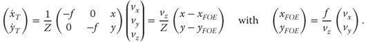

where f is the focal length of the camera, x and y are the image coordinates of a point in space (X,Y,Z) projected on to the image plane, x_FOE and y_FOE are the image coordinates of the focus of expansion (FOE) of the vector field (which corresponds to heading during forward translation), v_x is velocity (in space, not in the image) along the x axis, v_y is the velocity along the y axis, v_z is the velocity along the z-axis, Z is the position of the object measured along the z-axis (depth), and and are the image velocity in x and y coordinates, respectively.

Optic flow provides a rich set of cues for visually guided navigation, including:

1. Self-motion of the observer

2. TTC with surfaces/objects in the environment

3. Object segmentation and trajectories

4. Object deformations and morphing

Animals move to actively obtain visual information, and this information is utilized through movements of head, eyes, and body, which in turn generates new visual information. Many robots and unmanned vehicles are built with the same capabilities, primarily to optimize the use of sensor and computational resources through active vision [4]. In this chapter, we simplify the discussion of optic flow analysis by assuming that the eye is fixed in body-centric coordinates in order that we can focus on reactive visual navigation rather than eye or head movements. We justify this simplification through the fact that the effect of rotations can be estimated, and removed, either with extraretinal signals or from optic flow itself provided there is sufficient depth structure.

If we assume that there is no rotation of the eye/head/sensor, then the relative motion between the eye and the world is caused only by body motion. This body motion can be modeled through a 3D translational and 3D rotational velocity vector. Optic flow is estimated from the projection of those translational and rotational vectors on to the retina/sensor. Analysis of optic flow allows for the estimation of the 3D translational direction and 3D rotation velocity from the visual input stream. Note that 3D translational speed cannot be recovered due to the inherent size/distance ambiguity of a 2D projection of a 3D world, the object could be small and close by or large and far away. However, TTC can be recovered from the image stream and provides a behaviorally relevant measure of the relative distance to objects in the scene. Note that some authors (e.g., [5] Eq. (2.13)) derive temporal measures of distance (range/range rate) in their analysis but refer to them as relative depth rather than TTC. This omission is perhaps because they did not perform the final computation to put the measure into standard units of time or perhaps to avoid potential confusion with the definition of TTC (see Section 4).

Accurate TTC requires an estimate of the current direction of travel, which for the purposes of this chapter we define as heading. Heading can be estimated from optic flow or from an inertial sensor, although it should be noted that in practice mapping inertial heading estimates into the image frame often adds significant synchronization and calibration issues. TTC from optic flow provides a dense map of the relative distances to surfaces and objects in the scene. By dense, we mean that each sample location in the image is assigned a TTC value. For most applications, sample location is synonymous with pixel location. This dense map can serve as a rough sketch of objects, the volume of a scene, and provides information about empty, drivable space – this is also the basis of structure from motion algorithms, which are not discussed here. In applications where the speed of the sensor is known (e.g., a robot which measures its own speed), TTC multiplied by own speed provides an estimate of the true distance to static objects. Depending on what assumptions can be made with respect to object speed or size, it is also possible to estimate the distance to moving objects in some circumstances.

Optic flow can be used to segment both static and moving objects. In the moving object case, the directions and speeds of the vector field in the region of the object are inconsistent with the surrounding vector field generated by self-motion. Static object boundaries typically coincide with depth discontinuities – an object is in front of (or behind) another object. Due to the projective geometry of camera or models for image formation of the eye close versus far objects will have different image velocities. For instance, if there are two objects, one at 5 m distance and one at 10 m distance, and the camera moves to the left, the optic flow vectors from the closer object will have twice the speed compared to the speed of vectors from the far object. These speed discontinuities (that do not affect vector direction/angle) in optic flow indicate a depth discontinuity in the real world. For instance, a desk in front of the wall or a mug on the table introduces such discontinuities when moving relative to them. This phenomenon is commonly called motion parallax – closer objects move faster on your retina than those further away. A speed discontinuity in the optic flow can be detected and interpreted as object boundary. Motion parallax can be used to gain a depth ordering between objects which appear overlapping or connected within the visual field. Thus, optic flow not only facilitates the detection of edges of objects but also allows for the creation of a depth ordering among connected objects. Information about objects and their depth ordering helps navigation based on readily available and always up-to-date information about the visual world. Depth ordering is not the same as estimating relative depth from TTC but is rather a quasi-independent depth measure, which provides a more robust representation of object ordering in the environment requiring only relatively accurate speed estimation and, unlike TTC, does not require knowledge of current heading.

For ease of discussion, in this chapter, we focus only on rigid (nondeforming) independently moving objects on straight-line trajectories. These simplifications are valid for the vast majority of visual navigation tasks involving vehicles and world structure and can be mitigated for tasks involving biological objects. These visual variables, self-motion, TTC, and object boundaries can be integrated to generate motor plans and actions for steering toward a goal, avoiding obstacles, or pursuing a moving goal (or target). For reactive navigation, biological systems tightly couple perception and action through reflexive visual responses and visual navigation in a cluttered world.

18.3 Estimation of Self-Motion: Knowing Where You Are Going

Knowing your current direction of travel is essential for navigation. During reactive navigation, objects are only obstacles if they impede your desired trajectory; otherwise, they are benign and sometimes helpful environmental structure.¹ Whether the current objective of the navigation is defined visually (e.g., the objective is to dock with, or intercept, a particular object) or nonvisually (e.g., to go north) current direction of travel must be known in order to measure deviation from that objective. We define the current direction of travel as self-motion, egomotion, or heading. For our purposes here (and as is common in the biological literature), we use these terms interchangeably while understanding that, depending on the vehicle in question, heading and direction of travel are not always the same. Moreover, we limit the definition to straight-line trajectories. A detailed discussion of the estimation of curvilinear trajectories, which we define as path, is beyond the scope of this chapter and is only briefly touched upon.

Heading in a rigid, static world is represented in optic flow through the FOE [1]. The FOE is the point in the image space from which all vectors originate. During forward translation, with a forward-facing camera, the FOE will usually be within the borders of the image frame. However, there are cases where the FOE may be located outside the borders of the image frame. In addition to the FOE, there is a corresponding focus of contraction (FOC) that occurs at the location at which all vectors converge, which for forward translation is usually behind you. Figure 18.1 shows a typical optic flow field for forward translation with a forward-facing camera. Since the FOE coincides with heading, we define the core problem of heading estimation as the localization of the FOE. Mathematically, knowledge of the FOE is also required to convert from an observed optic flow field to a TTC representation.

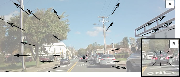
Figure 18.1 (a) Example optic flow field overlaid video from car driving forward past traffic on a public road, black circle indicates the focus of expansion and current heading. Image brightness has been increased and optic flow vectors have been sub-sampled and scaled for illustration. (b) Close up centered around the focus of expansion. The time to contact of the car, which we are heading towards, is encoded by the ratio of the optic flow vector magnitude to the distance of the origin of that vector from the FOE.

Optic flow fields corresponding to observer translations have been used as visual stimuli in many neurophysiological studies to determine if optic flow and the FOE could be used by primates for navigation. In primates, neurons in dorsal medial superior temporal area (MSTd) were found to be selective for radial expansion patterns – or in other words, they respond preferentially to translations with a particular heading [6, 7]. In this section, we begin with mathematical definitions before describing methods for estimating heading.

We assume that optic flow has been extracted from an image sequence. Formally, optic flow is defined as the vector field with x and y denoting Cartesian coordinates of the image position. Here, we focus on a model which describes this optic flow. First, we assume that the eye can be modeled by a pinhole camera with the focal length f that projects 3D points onto the 2D image plane . When modeling the human vision system, this is a simplistic assumption, resulting in some error, but works well for digital cameras, which are used in most real-world applications. Second, we assume that the observer is moving through a rigid environment, which is characterized by the distances Z(x,y) as seen through the pinhole camera at image location x and y. Third, we assume the observer's movement is described by the instantaneous 3D linear velocity and 3D rotational velocity . Formally, the model for optic flow is the visual image motion equation [5]

18.2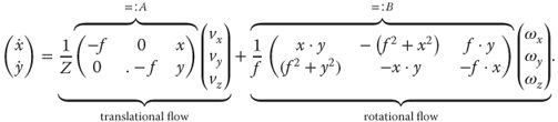

Each image location is assigned a flow vector , which is a velocity vector in the 2D image plane. These velocities express the movement of light intensity patterns within the image. When the observer moves in a static, rigid environment, Eq. (18.2) describes all these velocities. For a digital camera, we often associate the image locations with pixel locations and the flow vectors with “pixel velocities.” Analysis of Eq. (18.2) allows us to understand the impact of specific translations and rotations on optic flow fields, as shown in Figure 18.2.

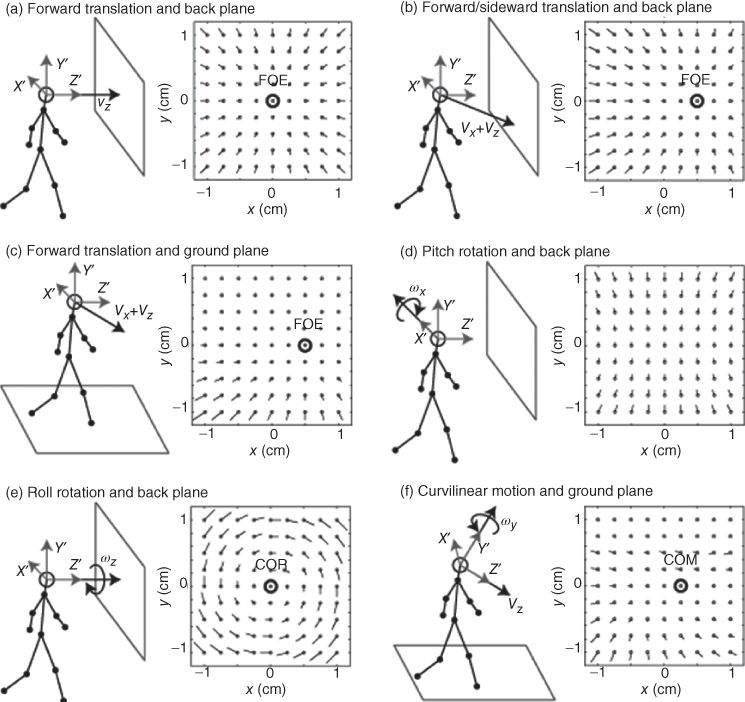
Figure 18.2 Characteristic optic flow patterns generated for observer motions toward a back plane or when walking along a ground plane. a) Flow for straight ahead translation toward a back plane at 10 m distance. b) Flow for the translation components vx = 0.45m/sec, vy = 0m/sec, and vz = 0.89m/sec toward a back plane at 10 m distance. c) The same translation as in b) but now above a ground plane. The angle between the line of sight and ground plane is 30 degrees and the distance of the ground plane measured along this line of sight is -10 meters. In these three cases a)-c) the focus of expansion (FOE) indicates the direction of travel in image coordinates. d) Flow for the pitch rotation of ωx = 3°/sec. e) Flow for the roll rotation of ωz = 9°/sec. In this case, the center of rotation (COR) appears at the image coordinates (0, 0). f) Flow for curvilinear motion with the translation components vx = 0.71m/sec, vy = 0m/sec, and vz = 0.71m/sec, and the rotational components ωx = 0°/sec, ωy = 3°/sec, and ωy = 0°/sec above the ground plane like in c). The center of motion (COM) marks the position of zero length vectors. All flow patterns are generated using the model Eq. (18.2).

Equation (18.2) allows us to understand how we can estimate the FOE (heading) from observed optic flow. If we simplify the problem by assuming that there are no rotations between measurements, and that we want an estimate of the FOE in image coordinates, then we can define a least-squares solution to find the intersection point of all of the motion vectors on the image plane. This problem can be posed using the standard matrix formulation of the form and solved in the least-squares sense using the pseudoinverse, . If we define , , and , then we can construct the solution as follows:

18.3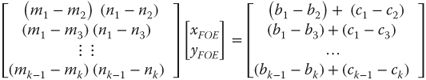

where and are the observed velocities at the location defined by x, and y, k is the total number of optic flow vectors. The visual angle of the FOE on the image plane corresponds to the current bearing angle, and this is often sufficient as a heading estimate for many applications, including TTC estimation which requires only the pixel coordinates of the FOE. This mathematical formulation continues to work when the FOE is outside the image plane, in practice, however, error will increase as the FOE gets further from the center of the image plane.

In a more general sense, we can formulate an optimization problem to estimate the translational and rotational motion and environmental structure that caused the observed optic flow pattern. Equation (18.4) poses one such nonlinear optimization problem that can be solved through gradient descent [8]:

18.4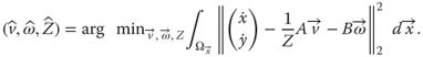

In Eq. (18.4), we use the estimated optic flow and subtract the model flow defined by Eq. (18.2). This results in a residual vector, which we take the Euclidean norm of. Assuming that the self-motion parameters are the same within the entire image plane we integrate over the area . This means, we have to estimate the model parameters , , and , whereas parameter can be different for each image location. We minimize the residual value, the difference between estimate and model, if we look for the minimum in the space of these parameters.

More details on the estimation of self-motion and a comparison between different methods are given in [9].

As noted previously, bioinspired methods are supported by neurophysiological data from primate brain area MST [6, 7]. Rather than taking a gradient descent approach or analytical treatment, the solution is found by sampling all reasonable motions and together with all reasonable depths Z and to evaluate a bioinspired likelihood function for these parameters [10, 11]. Each of these constructed sample optic flow patterns defines a template which represents travel in a particular direction. Self-motion is estimated by finding the template that best matches the observed optic flow field. The match score can be defined as a simple inner product between the template and the observed optic flow, normalized by the overall energy (sum of vector magnitudes) of the observed optic flow, or by using a standard correlation measure. Other hybrid approaches use optimization and sampling strategies [12–14]. Many biological template match methods reduce the large sample space by sampling (generating templates for) only a subset of possible self-motions. For example, the model in [10] samples only fixating self-motion. The ViSTARS model [15–18] computes heading in model MSTd using an inner product between the optic flow estimate in MT with a set of templates represented in the weight matrices connecting MT with MSTd. Each template corresponds to motion in a particular direction, with approximately 1° spacing horizontally and approximately 5° spacing vertically. In later work, ViSTARS was updated to define the templates to simultaneously calculate TTC and heading through the same computation. This has the benefit of eliminating all peripheral scaling bias² and thereby equally weighting all components of the optic flow field in the heading estimate. ViSTARS can tolerate small amounts of uncorrected rotation in the optic flow field but requires additional information about eye/camera rotations to estimate heading while the camera is panning. The template matching in ViSTARS is highly robust to noise in the optic flow field through the spatiotemporal smoothing that occurs at each processing stage of the model. This system-level smoothing, in space and time, emerges naturally from model neurons parameterized based on the documented properties of V1, MT, and MST cells. ViSTARS produces heading estimates that are consistent with human and primate heading estimation data, including in the presence of independently moving objects (which violate the mathematical assumptions of a static world), and are consistent with the temporal evolution of signals in MT and MSTd. The ViSTARS templates have recently been extended to incorporate spiral templates which are a closer match to primate neural data and enable the explanation of human curvilinear path estimation data [18].

Royden [19] presented a model of heading estimation based on a differential motion representation in primate MT. In a rigid world, differencing neighboring vectors in space results in a new vector with an arbitrary magnitude but that still converges on the FOE [20]. The chief benefit of using differential motion vectors is the simultaneous removal of rotation from the optic flow field. From the differential motion field, either a template match or a least-squares solution can be used to find the FOE. Heading estimates from Royden's modeling work yield similar heading estimation performance to humans in similar environments including in the presence of independently moving objects.

In summary, heading is directly observable from an optic flow field through estimation of the location of the FOE. There are a number of mathematical abstractions used throughout the biological and engineering literature; however, they can generally be placed in one of two groups: template matching and linear/nonlinear optimization problems (for a summary review, see [9]).

18.4 Object Detection: Understanding What Is in Your Way

Reactive navigation is by definition a behavioral response to the existence of unexpected objects along the desired trajectory. Therefore, object detection is a major component of reactive navigation. Note though that object identification and classification are not necessary. The fact that there is an object on the current trajectory is sufficient information to initiate an avoidance maneuver. In some applications, certain objects may pose a more serious obstacle than others, which requires some element of object identification or classification, but that is beyond the scope of this chapter. When a camera moves through the environment, optic flow can be extracted from the image plane. In a rigid, static world, the direction of all of those vectors has a common origin at the FOE, but the magnitude is a function of relative distance.³The boundaries of obstacles can be found by looking for depth discontinuities in the optic flow field – regions where neighboring pixels have significantly different vector magnitudes. Note that the word object is defined here in terms of how it impacts navigation, it may consist of multiple individual objects, or it may be a part of a larger object. Moving obstacles will also exhibit motion discontinuities, and the direction of the motion vectors corresponding to the moving object will point to a unique object FOE specific to that object. This object FOE can be used to determine the relative trajectory of the object with respect to the observer's trajectory. Finally, the interior (space between edges) of objects will, by definition, be a region of the image that produces no strong discontinuities. In other words, the interior of an object will have uniform or slowly varying vector magnitudes.

In this section, we define the local segmentation cues: accretion/deletion, expansion/contraction, acceleration/deceleration, spatial curvature, and temporal curvature (Table 18.2, Figure 18.3).

Table 18.2 Analytical models for five segmentation cues for objects cues using optic flow. The optic flow of the object is denoted by , and the optic flow of the background is denoted by . The sign of these defined expressions has the interpretation as indicated in the left column

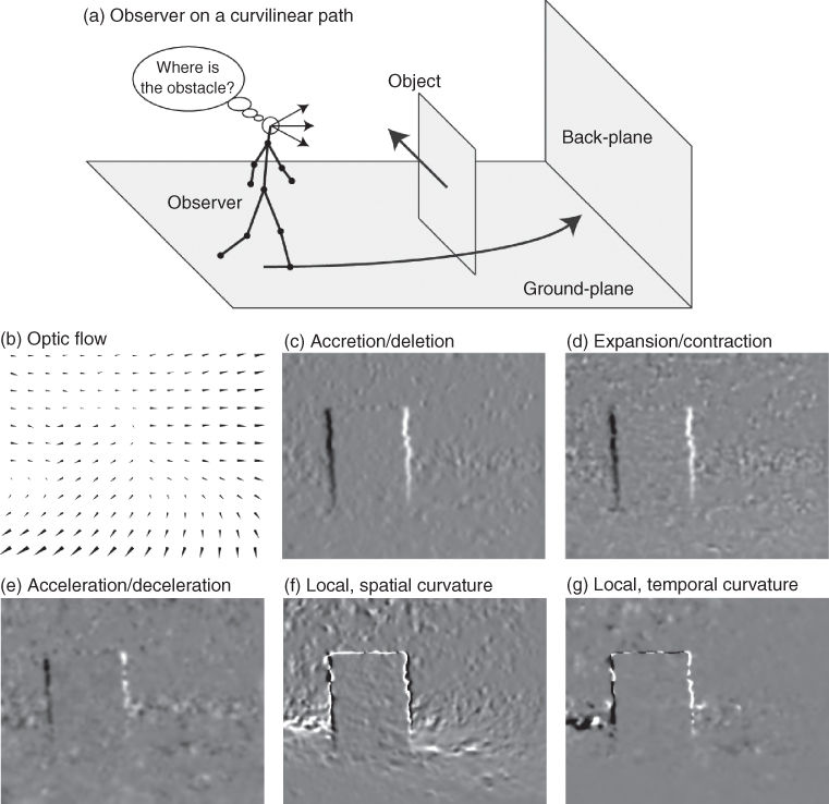
Figure 18.3 Segmentation cues for observer on a curvilinear path going around an independently moving object. a) Outline of motions. b) Estimated flow (Zach et al., [21]). c) Accretion (>0) and deletion (<0) cue. d) Expansion (>0) and contraction (<0) cue. e) Acceleration (>0) and deceleration (<0) cue. f) Local, spatial curvature cue. g) Local, temporal curvature cue. For curvature the sign indicates a concave (>0) or a convex (<0) curvature.

Accretion and deletion are expressed with respect to the angle β, which is the angle of the normal to the object's edge in the 2D image plane. Accretion (Δ > 0) denotes the uncovering of background by the object, and deletion happens when the object covers the background (Δ < 0). The unit of accretion and deletion is m/s.

We define expansion and contraction using spatial derivatives of optic flow. For forward self-motion, an expansion (δ > 0) indicates that the object is in front of the background. For a backward self-motion, the object appears behind the background, for example, when looking through an open door in the back wall. Assuming forward self-motion, a contraction (δ < 0) indicates that the object is behind the background. The unit of expansion and contraction is 1/s or Hz.

Acceleration and deceleration use the temporal dependency of the optic flow computing second-order temporal derivatives. This cue indicates acceleration for α > 0 and it indicates deceleration for α < 0. These accelerations and decelerations have the same interpretation as for objects in classical physics; however, here, the objects are patches of light in the image plane. The unit of this cue is m/s².

A combination of spatial derivatives of optic flow and the optic flow itself allows for the construction of a local curve, which approximates the characteristics of the optic flow, locally. This curvature is zero in cases where the spatial derivatives of the optic flow evaluate all to zero. For instance, translational self-motion toward a parallel backplane provides no curvature. However, if rotational self-motion is present, curvature is present. In general, the corresponding curve has a concave shape for ϑ > 0 and a convex shape for ϑ < 0. The unit of this spatial curvature is 1/m.

Instead of defining curvature in the image plane, an alternative is to define curvature in the temporal domain. Looking at one fixed location in the image plane, we define a curve through the two components of optic flow which change over time. This curve has a concave shape for γ > 0 and a convex shape for γ < 0. The unit for this temporal curvature is 1/m.

These five cues describe the segmentation between object and background [22]. They can also be derived from observed optic flow through calculation of the spatial and temporal derivatives and the expressions from Eqs. (18.5) to (18.9) substituting the terms (Figure 18.3). In practice, the use of derivatives on measured optic flow can result in noisy information.

Neurophysiological evidence suggests that subsets of cells in primate brain area MT respond to motion boundaries [23] through cells that respond most strongly to differences in estimated motion between two lobes of the receptive field. Differential motion cells are analogous to simple cells in V1 but look for differences in motion rather than differences in intensity. These differential motion cells project to ventral medial superior temporal (MSTv). The ViSTARS model segments objects using differential motion filters located in model MT, and the differential motion filters are grouped into object representations in model MSTv. These representations were demonstrated sufficient to match key human reactive navigation data.

Recent extensions to the ViSTARS model include the introduction of space-variant normalization across the differential motion filters. This provides more robust and reliable cell responses across the visual field and is more consistent with the space-variant representations in human and primate visual systems, for example, the log-polar representation in V1. This is implemented in such a way that each vector is normalized by its distance from the FOE; in other words, it is converted into expansion rate (mathematically defined as the reciprocal of TTC – see TTC section in the following text). Specifically, the optic flow vector field is converted to polar coordinates (r, θ), where r is the magnitude of the vector and theta is the angle from the origin (at the FOE). In each pixel location, the differences between a center (5 × 5 pixels) and surround filter (49 × 49 pixels) are calculated:

18.10

18.11

where subscripts d, c, and s denote the difference, center, and surround, respectively, and []⁺ denotes half-wave rectification (max(x,0)). The magnitude difference is then arbitrarily scaled by the distance from the FOE, D:

18.12

The step defined by Eq. (18.12) incorporates an arbitrary scaling parameter (1000) applied to the expansion rate at that location in space; the scaling parameter should be chosen taking into account the frame rate of the system and the expected range of observed expansion rates. Finally, both the angle and magnitude are thresholded, and the conjunction is defined as the output of the differential motion filter O:

18.13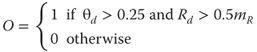

where m_R is the mean of all of the R_d values within the current image and the parameters 0.25 and 0.5 are chosen based on the desired sensitivity of the filter. Equations (18.10)–(18.13) are simplifications of the ViSTARS dynamical models of differential cells in MT (the full biological motivation and mathematical definition is described in [16]) modified through space-variant scaling to eliminate peripheral bias.

Peripheral bias is the phenomenon that motion vector magnitude further from the FOE is larger, for objects the same distance away, than for motion vectors closer to the FOE. Space-variant normalization (Eq. (18.12)) reduces the dynamic range required to analyze motion across the optic flow field by eliminating peripheral bias. The net effect of this space-variant normalization is that small, slow-moving objects can be accurately segmented from a moving wide field of view imager irrespective of where on the image plane they are projected (Figure 18.4).

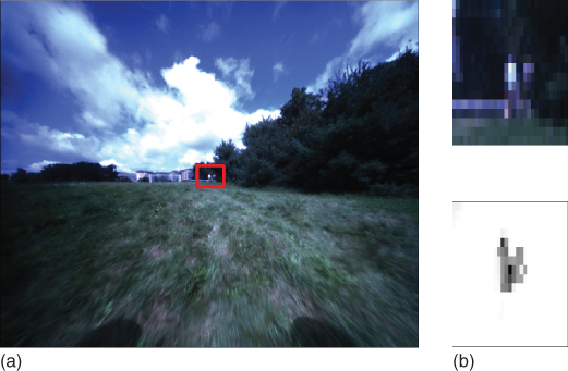
Figure 18.4 ViSTARS can segment small, slow-moving objects from a moving wide field of view imager through space-variant differential motion processing. (a) The camera is moving forward at around 4 m/s (10 mph), two people are walking to the right (red box). (b)Space-variant differential motion accurately segments the people.

In summary, knowing the object identity is not necessary for reactive navigation. Objects can be detected in optic flow through analysis of optic flow and specifically through differentiation of the motion field which results in motion boundaries corresponding to depth discontinuities in space.

18.5 Estimation of TTC: Time Constraints from the Expansion Rate

As noted in previous sections, optic flow does not carry sufficient information to determine the distance to objects or surfaces in the observed scene. This is due to the size/distance ambiguity – a small object at a short distance is projected on to the retina/eye/sensor exactly the same as a large object at a far distance.

By contrast, the expansion rate of an object – when defined as a with w being the size of the object in the image plane (width, height, area) – is the reciprocal of the ratio of distance to closing speed, which is the TTC (, TTC): mathematically, . Note that although is often defined in the biological literature using angular size, this mathematical equivalence is only approximately true when using angular sizes. Moreover, the term “expansion rate” is often used to refer to the change in object size rather than as a ratio (as defined previously); this is not mathematically speaking a rate unless it is defined as a ratio against some other quantity (although one could argue that it is implicitly the ratio per unit of time between image frames). The definition of expansion rate as the ratio of “change in size” to “size” is critical to understanding and exploiting the relationship between TTC and object size growth on the image plane. It allows us to mathematically prove that expansion rate, E = 1/TTC which in turn allows us to infer, for example, that a 20% expansion rate per second is exactly equal to a 5 s TTC. These relationships are easily derived using perspective projection [17] and provide a robust representation for visual navigation.

The definition of TTC is the time until an object passes the infinite plane parallel to the image plane passing through the camera focal point. TTC does not indicate anything about the likelihood of a collision with an object. When combined with information on the trajectory of an object, for example, using bearing information to determine that an object is on a collision trajectory, TTC is the time-to-collision. Note the important difference between contact and collision in this context. When an object is not on a collision trajectory, TTC is the time to pass by the object. This mathematically abstract definition of TTC can be a source of confusion, which may be why some authors have used the term relative depth instead – particularly when talking about static environments.

Optic flow defines motion of a point on the image plane from one time to another relative to a FOE/contraction, and so TTC can be computed from optic flow as follows (Figure 18.5):

18.14

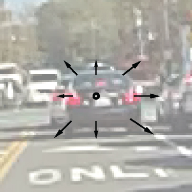
Figure 18.5 Close-up centered around the focus of expansion from Figure 18.1. The time to contact of the car, which we are heading toward, is encoded by the ratio of the optic flow vector magnitude to the distance of the origin of that vector from the FOE.

Self-motion creates an FOE, which allows for a simple transformation from optic flow to a dense TTC (relative depth) map of environmental structure. For parallel trajectories, the FOE is at infinity, and in this case, TTC is also infinity. Before discussing the application of TTC for visual navigation, it is important to understand the assumptions that go into the derivation of TTC from visual information:

1. The world is rigid (nondeforming).

2. The observer (camera) is traveling on a straight-line trajectory (between measurements).

3. The observer (camera) is traveling at a fixed speed (between measurements).

4. If the world contains one or more independently moving objects:

a. The motion vectors from those objects are analyzed with respect to their own object's FOE.

b. The object is moving on a straight-line trajectory relative to the observer.

c. The object is traveling at a fixed speed relative to the observer.

Assumption 1 is violated when the field of view contains objects that are constantly changing their shape, such as jelly fish, or that are deforming due to external forces, such as trees blowing in the wind. For realistic viewing conditions, these motions rarely occur. Even if they appear, the motions introduced by such deformations are small compared to the motion due to translation of the sensor. As a result, the error introduced by these deformations is small. Moreover, if TTC is estimated in a filter, these deformation motions will tend to smooth out, and error will be extremely small compared to measurement error in general.

Assumption 2 is violated whenever the observer changes direction. The TTC coordinate frame is inherently body based, when the body turns, so does the coordinate frame – and therefore the plane to which TTC relates. This would be true of a distance metric also; however, a distance-based coordinate frame can be rotated relatively easily, and a direction-based coordinate frame, such as TTC, is more complex. As with assumption 1, if TTC is being estimated in a filter and the changes in trajectory are smooth, then the TTC estimates will automatically update as trajectory changes. This means that it is essential that TTC be conceptualized as a dynamic visual variable that changes in response to observer behaviors.

Assumption 3 is violated when the observer changes speed. This is obvious that if you start moving faster toward something, then the TTC changes; therefore, any process that estimates TTC must assume that there was a constant speed between the image measurements that were used to estimate optic flow. As with assumptions 1 and 2, provided TTC is estimated in a filter and speed changes are smooth, then TTC estimates will be automatically updated as the speed changes.

Assumption 4 relates to independently moving objects which create their own FOE. Just as the observer's FOE provides information about heading and TTC, so does the object's FOE:

1. IF the object's FOE lies within the boundary of the object

2. THEN the object is likely to be on a direct collision course

3. IF the object's FOE lies outside the boundary of the object

4. THEN the object is not likely to be on a collision course

However, reliably measuring the FOE of an object is nontrivial, particularly when the camera is on a moving, vibrating vehicle, and the object appears small in the image. As a result, it is often more reliable and robust to assume the FOE is at the center of the object to estimate TTC rather than estimate the FOE. The error introduced by this FOE assumption can be computed and it can be minimized by using a dense TTC map across the whole object and averaging to provide object TTC. The resulting TTC error is high for objects not on a collision course but error becomes close to zero for objects on a direct collision course. This assumption thereby provides accurate behaviorally relevant information for navigation but would not be suitable for the application of object tracking. Note that assumptions relating to fixed-line trajectories and fixed speeds of moving objects are the same as for the moving object case and the same explanations and mitigations apply. Rather than using the object's FOE to determine collision likelihood, it is often more reliable to use the 2D object trajectory on the image plane and an alternate (nonoptic flow based) analysis, for example, constant bearing strategy or an image movement-based tracking model.

TTC (and expansion/looming) responsive cells have been observed in many animals from locusts to frogs and to pigeons, with pigeons being the most studied. In primates, the receptive fields of MST cells are particularly suited for the estimation of TTC [17], although there is evidence for TTC response in higher areas as well.

The ViSTARS model incorporates TTC estimation directly into model MSTd cells, simultaneously solving for FOE and TTC. This is performed through a redefinition of the heading templates to normalize each motion vector by its distance from the corresponding template FOE. This allows the template to simultaneously locate the FOE and estimate the average TTC to objects within the span of the template. The templates are mathematically defined to equally weigh each optic flow vector, irrespective of its location on the image plane, as a function of expansion rate. This means that heading estimation equally weights the center region and the periphery, and that the template match score is proportional to the mean TTC of the object(s) within the receptive field of the cell [17].

The ViSTARS TTC template definition provides all of the information necessary to reproject the optic flow into a dense TTC map, which can then be fed directly into a steering field. Simply multiply each component of the winning template (the template with the maximal response when matched against optic flow), with the observed optic flow, and the result is a spatial representation of the world where the magnitude of the response at each location is proportional to the expansion rate at that location. In other words, the winning template provides a scale factor for each pixel location that will convert the optic flow representation into an expansion rate (1/TTC) representation. When combined with object boundaries from object segmentation (see previous section), this provides a complete representation of space to facilitate reactive obstacle avoidance.

In summary, TTC can be extracted directly from optic flow, assuming the location of the FOE is known. TTC, and its reciprocal expansion rate, provides relevant behavioral information as to the imminence of collision with any object and are a robust way to measure relative distances from optic flow. Moreover, representation of the world as a function of TTC (e.g., as expansion rate) directly facilitates reactive navigation behaviors.

18.6 Steering Control: The Importance of Representation

The biological basis of steering control in higher mammals has not yet been discovered. This chapter is primarily concerned about biological inspiration for applied visual reactive control. In this section, we discuss how the visual representations observed in primate brain (and discussed previously) can be efficiently combined for reactive navigation in a biologically plausible computational framework.

Steering is the manifestation of reactive navigation through behavioral modification. When an obstacle is detected, the observer must change trajectory to avoid it. When the current trajectory is not on an intercept path with the goal object/location/direction, the observer must change trajectory. Steering can therefore be thought of as a decision-making process or a cognitive process. The steering process must analyze the visual variables, heading, visual angle and TTC of the obstacle, and visual angle and TTC of the goal, to determine an appropriate trajectory avoiding collision with obstacles while navigating toward the goal.

The chosen representation for these visual variables constrains the space of possible solutions. It seems likely that the brain represents these variables in a spatial map [24]. In a spatial map, each unique position in space has a corresponding unique position in the map. In ViSTARS and related models, TTC is represented through the magnitude of activation at any given point in the 2D map. Three 2D maps are required for reactive navigation. The first represents heading, the second represents one or more obstacles, and the third represents the goal; more representations could be incorporated to fuse additional information such as attention and auditory information. The precursor model to ViSTARS [24] showed how three representations such as these could be minimally combined to produce a steering field [25], whereby the magnitude of activation at any given location defines the navigability of that location. The maxima in the representation defines the desired trajectory.

Figure 18.6 illustrates how the obstacle and goal representations are generated from projection of objects into the steering field in ViSTARS through a 1D example. A key requirement here is that the activation around an object's boundary should reduce in amplitude as a function of distance of this object boundary to the camera location in a logarithmic manner. This distance dependency is a key feature of ViSTARS object representations.

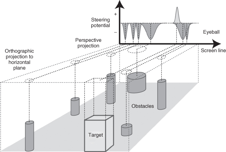
Figure 18.6 Illustration of how representations of the goal (target) and obstacles are combined into the steering field in ViSTARS. The obstacle representation is inverted to create minima in regions where navigation will result in a collision. This is added to the target representation to create a maximum at the point in space that will safely avoid the obstacles while still heading toward the goal.

The obstacle representation is inverted to create minima in regions where navigation will result in a collision. The obstacle representation is summed with the goal representation to create the steering field (not shown) with maxima at locations that will safely avoid the obstacles. The global maximum in the steering field defines the trajectory that will head toward the goal while avoiding the obstacles, directly defining where the observer should steer toward.

When applied to the constraints of a robot, the control mechanism will be specific to the vehicle and application, but in most cases, the controller will make trajectory modifications to align the current heading with the closest maxima in the steering field. To provide temporal stability (damping) in the steering field, the current heading estimate can be added into the steering field (as it was in the ViSTARS publications), but in most cases, damping can be handled within the vehicle controller itself.

The ViSTARS steering field is similar to a potential field control law in that it creates attractors and repellers, which are used to generate trajectories. However, unlike a potential field controller, the steering field is based on a first person perspective view of the environment extracted in real time during navigation and does not require a priori information as to the location of objects within the environment. As such, it does not rely on any memorized locations and is entirely based on the current observation of obstacles and goal from an egocentric viewpoint. ViSTARS, and its precursor STARS, demonstrated how trajectories generated with this steering field were qualitatively and quantitatively similar to those produced by humans in similar environments.

It is worth noting that [26] utilizes a very similar steering field in a spike-latency model for sonar-based navigation in an algorithm called “Openspace,” and so the representation of goals and obstacles as distributions across navigable space may also provide a multimodal reactive navigation capability.

18.7 Conclusions

This chapter provided an analysis of the relevant visual representations and variables required to support reactive visual navigation: self-motion, object boundaries, TTC/relative depth, and steering decisions. Likely, mappings of these representations to the magnocellular pathway of the primate visual system are shown in Table 18.1. Other animals, including insects, have different but often comparable circuits involved in the computation of these visual variables (see Chapter 17 about how elementary motion detectors are used by insects). A recent review [27] provides details of these representations in the visual system of honeybees. Biological systems tightly integrate visual perception with the motor system to allow for rapid reactive navigation in a changing world. Understanding the detailed representations within the primate brain may allow us to build robotic systems with the same capabilities. Basic biological capabilities like reactive navigation are fundamental for the integration of robotics into our daily lives and in the automation of highly dangerous tasks such as firefighting, search and rescue, and so on.

More information about the mathematical models (including code) described in this chapter, along with related work, can be found on http://opticflow.bu.edu, http://vislab.bu.edu, and http://vislab.bu.edu/projects/vistars/.

Acknowledgments

NAB was supported in part by the Office of Naval Research (ONR) N00014-11-1-0535 and Scientific Systems Company Inc. FR was supported in part by CELEST, a National Science Foundation Science (NSF) of Learning Center (NSF SMA-0835976), NSF BCS-1147440, the ONR N00014-11-1-0535, and ONR MURI N00014-10-1-0936.

References

1. 1. Gibson, J.J. (1950) The Perception of the Visual World, Houghton Mifflin, Boston.

2. 2. Raudies, F. (2013) Optic flow. Scholarpedia, 8 (7), 30724.

3. 3. Scharstein, D. http://vision.middlebury.edu/flow/eval/ (accessed 13 April 2015)

4. 4. Aloimonos, J., Weiss, I., and Bandyopadhyay, A. (1988) Active vision. Int. J. Comput. Vision, 2, 333–356.

5. 5. Longuet-Higgins, H.C. and Prazdny, K. (1980) The interpretation of a moving retinal image. Proc. R. Soc. Lond. B Biol. Sci., 208, 385–397.

6. 6. Tanaka, K., Hikosaka, K., Saito, H., Yukie, M., Fukada, Y., and Iwai, E. (1986) Analysis of local and wide-field movements in the superior temporal visual areas of the macaque monkeys. J. Neurosci., 6(1), 134–144.

7. 7. Duffy, C.D. and Wurtz, R.H. (1995) Response of monkey MST neurons to optic flow stimuli with shifted centers of motion. J. Neurosci., 15 (7), 5192–5208.

8. 8. Soatto, S. (2000) Optimal structure from motion: local ambiguities and global estimates. Int. J. Comput. Vision, 39 (3), 195–228.

9. 9. Raudies, F. and Neumann, H. (2012) A review and evaluation of methods estimating ego-motion. Comput. Vision Image Understanding, 116 (5), 606–633.

10.10. Perrone, J.A. and Stone, L.S. (1994) A model of self-motion estimation within primate extrastriate visual cortex. Vision Res., 34 (21), 2917–2938.

11.11. Perrone, J.A. (1992) Model for the computation of self-motion in biological systems. J. Opt. Soc. Am. A, 9 (2), 177–192.

12.12. Jepson, A. and Heeger, D. (1992) Linear Subspace Methods for Recovering Translational Direction. Technical Report RBCV-TR-92-40, University of Toronto, Department of Computer Science, Toronto.

13.13. Lappe, M. and Rauschecker, J. (1993) A neural network for the processing of optic flow from ego-motion in man and higher mammals. Neural Comput., 5, 374–391.

14.14. Lappe, M. (1998) A model of the combination of optic flow and extraretinal eye movement signals in primate extrastriate visual cortex – neural model of self-motion from optic flow and extraretinal cues. Neural Networks, 11, 397–414.

15.15. Browning, N.A., Mingolla, E., and Grossberg, S. (2009) A neural model of how the brain computes heading from optic flow in realistic scenes. Cogn. Psychol., 59 (4), 320–356.

16.16. Browning, N.A., Grossberg, S., and Mingolla, E. (2009) Cortical dynamics of navigation and steering in natural scenes: motion-based object segmentation, heading, and obstacle avoidance. Neural Networks, 22 (10), 1383–1398.

17.17. Browning, N.A. (2012) A neural circuit for robust time-to-contact estimation based on primate MST. Neural Comput., 24 (11), 2946–63.

18.18. Layton, O.W. and Browning, N.A. (2014) A unified model of heading and path perception in primate MSTd. PLoS Comput. Biol., 10 (2), e1003476. doi: 10.1371/journal.pcbi.1003476

19.19. Royden, C.S. (2002) Computing heading in the presence of moving objects: a model that uses motion-opponent operators. Vision Res., 42 (28), 3043–58.

20.20. Rieger, J. and Lawton, D.T. (1985) Processing differential image motion. J. Opt. Soc. Am., 2 (2), 354–359.

21.21. Zach, C., Pock, T., and Bischof, H. (2007) A duality based approach for realtime TV-L optical flow. Hamprecht, F.A., Schnörr, C., and Jähne, B. (Eds.): DAGM 2007, Lecture Notes in Computer Science, 4713, Springer, Heidelberg, pp. 214–223

22.22. Raudies, F. and Neumann, H. (2013) Modeling heading and path perception from optic flow in the case of independently moving objects. Front. Behav. Neurosci., 7, 23. doi: 10.3389/fnbeh.2013.00023

23.23. Born, R.T. and Bradley, D.C. (2005) Structure and function of visual area MT. Annu. Rev. Neurosci., 28, 157–189.

24.24. Elder, D.M., Grossberg, S., and Mingolla, E. (2009) A neural model of visually guided steering, obstacle avoidance, and route selection. J. Exp. Psychol.: Hum. Percept. Perform., 35 (5), 1501.

25.25. Schöner, G., Dose, M., and Engels, C. (1995) Dynamics of Rob. Autom Syst., 16, 213–245.

26.26. Horiuchi, T.K. (2009) A spike-latency model for sonar-based navigation in obstacle fields. IEEE Trans. Circuits Syst. I, 56 (11), 2393–2401.

27.27. Srinivasan, M.V. (2011) Honeybees as a model for the study of visually guided flight, navigation and biologically inspired robotics. Physiol. Rev., 91, 413–460.

¹ In more complex environments where objects can pose a threat based on their identity (e.g., a sniper scope), then additional mechanisms are required to detect, identify, and characterize the threat.² Peripheral scaling bias is the phenomenon where during forward translation motion vector magnitude further from the FOE is larger than motion vector magnitude closer to the FOE.³ More accurately, it is a function of the reciprocal of TTC.