Computer Vision: Models, Learning, and Inference (2012)

This chapter provides a brief overview of modern preprocessing methods for computer vision. In Section 13.1 we introduce methods in which we replace each pixel in the image with a new value. Section 13.2 considers the problem of finding and characterizing edges, corners and interest points in images. In Section 13.3 we discuss visual descriptors; these are low-dimensional vectors that attempt to characterize the interesting aspects of an image region in a compact way. Finally, in Section 13.4 we discuss methods for dimensionality reduction.

13.1 Per-pixel transformations

We start our discussion of preprocessing with per-pixel operations: these methods return a single value corresponding to each pixel of the input image. We denote the original 2D array of pixel data as P, where p_ij is the element at the i^th of I rows and the j^th of J columns. The element p_ij is a scalar representing the grayscale intensity. Per-pixel operations return a new 2D array X of the same size as P containing elements x_ij.

13.1.1 Whitening

The goal of whitening (Figure 13.1) is to provide invariance to fluctuations in the mean intensity level and contrast of the image. Such variation may arise because of a change in ambient lighting intensity, the object reflectance, or the camera gain. To compensate for these factors, the image is transformed so that the resulting pixel values have zero mean and unit variance. To this end, we compute the mean μ and variance σ² of the original grayscale image P:

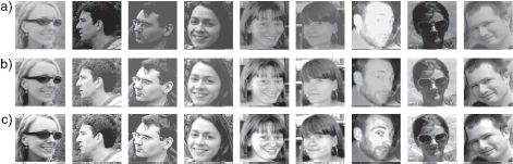
Figure 13.1 Whitening and histogram equalization. a) A number of faces which have been captured with widely varying contrasts and mean levels. b) After whitening, the images have the same mean and variance. c) After histogram equalization, all of the moments of the images are approximately the same. Both of these transformations reduce the amount of variation due to contrast and intensity changes.

These statistics are used to transform each pixel value separately so that

For color images, this operation may be carried out by computing the statistics μ and σ² from all three channels or by separately transforming each of the RGB channels based on their own statistics.

Note that even this simple transformation has the potential to hamper subsequent inference about the scene: depending on the task, the absolute intensities may or may not contain critical information. Even the simplest preprocessing methods must be applied with care.

13.1.2 Histogram equalization

The goal of histogram equalization (Figure 13.1c) is to modify the statistics of the intensity values so that all of their moments take predefined values. To this end, a nonlinear transformation is applied that forces the distribution of pixel intensities to be flat.

We first compute the histogram of the original intensities h where the k^th of K entries is given by

where the operation δ[•] returns one if the argument is zero and zero otherwise. We then cumulatively sum this histogram and normalize by the total number of pixels to compute the cumulative proportion c of pixels that are less than or equal to each intensity level:

Finally, we use the cumulative histogram as a look up table to compute the transformed value so that

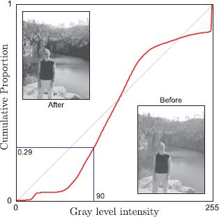
Figure 13.2 Histogram equalization. The abscissa indicates the pixel intensity. The ordinate indicates the proportion of intensities that were less than or equal to this value. This plot can be used as a look-up table for histogram equalizing the intensities. For a given intensity value on the abscissa, we choose the new intensity to be the maximum output intensity K times the value on the ordinate. After this transformation, the intensities are equally distributed. In the example image, many of the pixels are bright. Histogram equalization spreads these bright values out over a larger intensity range, and so has the effect of increasing the contrast in the brighter regions.

For example, in Figure 13.2 the value 90 will be mapped to K × 0.29 where K is the maximum intensity (usually 255). The result is a continuous number rather than a discretized pixel intensity but is in the same range as the original data. The result can be rounded to the nearest integer if subsequent processing demands.

13.1.3 Linear filtering

After filtering an image, the new pixel value x_ij consists of a weighted sum of the intensities of pixels in the surrounding area of the original image P. The weights are stored in a filter kernel F, which has entries f_m,n, where m ∈ {−M…M} and n ∈ {−N … N}.

More formally, when we apply a filter, we convolve the P with the filter F, where two-dimensional convolution is defined as

Notice that by convention, the filter is flipped in both directions so the top left of the filter f_−M,−N weights the pixel p_{i+M, j+N} to the right and below the current point in P. Many filters used in vision are symmetric in such a way that this flipping makes no practical difference.

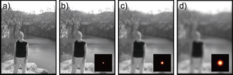
Figure 13.3 Image blurring. a) Original image. b) Result of convolving with a Gaussian filter (filter shown in bottom right of image). Each pixel in this image is a weighted sum of the surrounding pixels in the original image, where the weights are given by the filter. The result is that the image is slightly blurred. c-d) Convolving with a filter of increasing standard deviation causes the resulting image to be increasingly blurred.

Without further modification, this formulation will run into problems near the borders of the image: it needs to access points that are outside the image. One way to deal with this is to use zero padding in which it is assumed that the value of P is 0 outside the defined image region.

We now consider a number of common types of filter.

Gaussian (blurring) filter

To blur an image, we convolve it with a 2D Gaussian,

Each pixel in the resulting image is a weighted sum of the surrounding pixels, where the weights depend on the Gaussian profile: nearer pixels contribute relatively more to the final output. This process blurs the image, where the degree of blurring is dependent on the standard deviation σ of the Gaussian filter (Figure 13.3). This is a simple method to reduce noise in images taken at very low light levels.

First derivative filters and edge filters

A second use for image filtering is to locate places in the image where the intensity changes abruptly. Consider taking the first derivative of the image along the rows. We could approximate this operation by simply computing the difference between two offset pixels along the row. This operation can be accomplished by filtering with the operator F = [−1 0 1]. This filter gives zero response when the image is flat in the horizontal direction: it is hence invariant to constant additive luminance changes. It gives a negative response when the image values are increasing as we move in a horizontal direction and a positive response when they are decreasing (recall that convolution flips the filter by 180°). As such, it is selective for edges in the image.

The response to the filter F = [−1 0 1] is noisy because of its limited spatial extent. Consequently, slightly more sophisticated filters are used to find edges in practice. Examples include the Prewitt operators (Figures 13.4b-c)

and the Sobel operators

where in each case the filter F_x is a filter selective for edges in the horizontal direction, and F_y is a filter selective for edges in the vertical direction.

Laplacian filters

The Laplacian filter is the discrete two-dimensional approximation to the Laplacian operator ▿² and is given by

Applying the discretized filter F to an image results in a response of high magnitude where the image is changing, regardless of the direction of that change (Figure 13.4d): the response is zero in regions that are flat and significant where edges occur in the image. It is hence invariant to constant additive changes in luminance and useful for identifying interesting regions of the image.

Laplacian of Gaussian filters

In practice the Laplacian operator produces noisy results. A superior approach is to first smooth the image with a Gaussian filter and then apply the Laplacian. Due to the associative property of convolution, we can equivalently convolve the Laplacian filter by a Gaussian and apply the resulting Laplacian of Gaussian filter to the image (Figure 13.4e). This Laplacian of Gaussian has the advantage that it can be tuned to be selective for changes at different scales, depending on the scale of the Gaussian component.

Difference of Gaussians

The Laplacian of Gaussian filter is very well approximated by the difference of Gaussians filter (compare Figures 13.4e and 13.4f). As the name implies, this filter is created by taking the difference of two Gaussians at nearby scales. The same result can be achieved by filtering the image with the two Gaussians separately and taking the difference between the results. Again, this filter responds strongly in regions of the image that are changing at a predetermined scale.

Gabor filters

Gabor filters are selective for both scale and orientation. The 2D Gabor function is the product of a 2D Gaussian with a 2D sinusoid. It is parameterized by the covariance of the Gaussian and the phase , orientation ω, and wavelength λ of the sine wave. If the Gaussian component is spherical, it is defined by

where σ controls the scale of the spherical Gaussian. It is typical to make the wavelength proportional to the scale σ of the Gaussian so a constant number of cycles is visible.

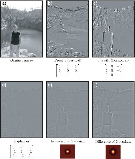
Figure 13.4 Image filtering with first- and second-derivative operators. a) Original image. b) Convolving with the vertical Prewitt filter produces a response that is proportional to the size and polarity of edges in the vertical direction. c) The horizontal Prewitt filter produces a response to edges in the horizontal direction. d) The Laplacian filter gives a significant response where the image changes rapidly regardless of direction. e) The Laplacian of Gaussian filter produces similar results but the output is smoothed and hence less noisy. f) The difference of Gaussians filter is a common approximation to the Laplacian of Gaussian.

The Gabor filter is selective for elements within the image at a certain frequency and orientation band and with a certain phase (Figure 13.5). It is invariant to constant additive changes in luminance when the sinusoidal component is asymmetric relative to the Gaussian. This is also nearly true for symmetric Gabor functions, as long as several cycles of the sinusoid are visible. A response that is independent of phase can easily be generated by squaring and summing the responses of two Gabor features with the same frequency, orientation, and scale, but with phases that are π/2 radians apart. The resulting quantity is termed the Gabor energy and is somewhat invariant to small displacements of the image.

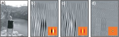
Figure 13.5 Filtering with Gabor functions. a) Original image. b) After filtering with horizontal asymmetric Gabor function at a large scale (filter shown bottom right). c) Result of filtering with horizontal symmetric Gabor function at a large scale. d) Response to diagonal Gabor filter (responds to diagonal changes).

Filtering with Gabor functions is motivated by mammalian visual perception: this is one of the first processing operations applied to visual data in the brain. Moreover, it is known from psychological studies that certain tasks (e.g., face detection) are predominantly dependent on information at intermediate frequencies. This may be because high-frequency filters see only a small image region and are hence noisy and relatively uninformative, and low-frequency filters act over a large region and respond disproportionately to slow changes due to lighting.

Haar-like filters

Haar-like filters consist of adjacent rectangular regions that are balanced so that the average filter value is zero, and they are invariant to constant luminance changes. Depending on the configuration of these regions, they may be similar to derivative or Gabor filters (Figure 13.6).

However, Haar-like filters are noisier than the filters they approximate: they have sharp edges between positive and negative regions and so moving by a single pixel near an edge may change the response significantly. This drawback is compensated for by the relative speed with which Haar functions can be computed.

To compute Haar-like functions rapidly, we first form the integral image (Figure 13.6g). This is an intermediate representation in which each pixel contains the sum of all of the intensity values above and to the left of the current position. So the value in the top-left corner is the original pixel value at that position and the value in the bottom-right corner is the sum of all of the pixel values in the image. The values in the other parts of the integral image are between these extremes.

Given the integral image I, it is possible to compute the sum of the intensities in any rectangular region with just four operations, regardless of how large this region is. Consider the region is defined by the range [i₀, i₁] down the columns and [j₀, j₁] along the rows. The sum S of the internal pixel intensities is

The logic behind this calculation is illustrated in Figure 13.6f-i.

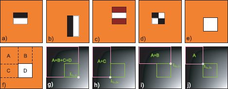
Figure 13.6 Haar-like filters. a-d) Haar-like filters consist of rectangular regions. Convolution with Haar-like filters can be done in constant time. e) To see why, consider the problem of filtering with this single rectangular region. f) We denote the sum of the pixel values in these four regions as A,B,C, and D. Our goal is to compute D. g) The integral image has a value that is the sum of the intensities of the pixels above and to the left of the current position. The integral image at position (i₁,j₁) hence has value A+B+C+D. h) The integral image at (i₁,j₀) has value A+C. i) The integral image at (i₀,j₁) has value A+B. j) The integral image at (i₀,j₀) has value A. The sum of the pixels in region D can now be computed as I_i1,j₁ + I_i0,j₀ − I_i1,j₀ − I_i0,j₁ = (A + B + C + D) + A − (A + C) − (A + B) = D. This requires just four operations regardless of the size of the original square region.

Since Haar-like filters are composed of rectangular regions, they can be computed using a similar trick. For a filter with two adjacent rectangular regions, six operations are required. With three adjacent rectangular regions, eight operations are required. When the filter dimensions M and N are large, this approach compares very favorably to a naïve implementation of conventional filtering which requires O(MN) operations to compute the filter response due to a M × N kernel. Haar filters are often used in real-time applications such as face detection because of the speed with which they can be computed.

13.1.4 Local binary patterns

The local binary patterns (LBP) operator returns a discrete value at each pixel that characterizes the local texture in a way that is partially invariant to luminance changes. For this reason, features based on local binary patterns are commonly used as a substrate for face recognition algorithms.

The basic LBP operator compares the eight neighboring pixel intensities to the center pixel intensity, assigning a 0 or a 1 to each neighbor depending on whether they are less than or greater than the center value. These binary values are then concatenated in a predetermined order and converted to a single decimal number that represents the “type” of local image structure (Figure 13.7).

With further processing, the LBP operator can be made orientation invariant: the binary representation is repeatedly subjected to bitwise shifts to create eight new binary values and the minimum of these values is chosen. This reduces the number of possible LBP values to 36. In practice, it has been found that the distribution over these 36 LBP values is dominated by those that are relatively uniform. In other words, binary strings where transitions are absent (e.g., 00000000, 11111111) or infrequent (e.g., 00001111, 00111111) occur most frequently. The number of texture classes can be further reduced by aggregating all of the nonuniform LBPs into a single class. Now the local image structure is categorized into nine LBP types (eight rotationally invariant uniform patterns and one nonuniform class).

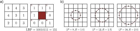
Figure 13.7 Local binary patterns. a) The local binary pattern is computed by comparing the central pixel to each of its eight neighbors. The binary value associated with each position is set to one if that neighbor is greater than or equal to the central pixel. The eight binary values can be read out and combined to make a single 8-bit number. b) Local binary patterns can be computed over larger areas by comparing the current pixels to the (interpolated) image at positions on a circle. This type of LBP is characterized by the number of samples P and the radius of the circle R.

The LBP operator can be extended to use neighborhoods of different sizes: the central pixel is compared to positions in a circular pattern (Figure 13.7b). In general, these positions do not exactly coincide with the pixel grid, and the intensity at these positions must be estimated using bilinear interpolation. This extended LBP operator can capture texture at different scales in the image.

13.1.5 Texton maps

The term texton stems from the study of human perception and refers to a primitive perceptual element of texture. In other words, it roughly occupies the role that a phoneme takes in speech recognition. In a machine vision context a texton is a discrete variable that designates which one of a finite number of possible texture classes is present in a region surrounding the current pixel. A texton map is an image in which the texton is computed at every pixel (Figure 13.8).

Texton assignment depends on training data. A bank of N filters is convolved with a set of training images. The responses are concatenated to form one N × 1 vector for each pixel position in each training image. These vectors are then clustered into K classes using the K-means algorithm (Section 13.4.4). Textons are computed for a new image by convolving it with the same filter bank. For each pixel, the texton is assigned by noting which cluster mean is closest to the N × 1 filter output vector associated with the current position.

The choice of filter bank seems to be relatively unimportant. One approach has been to use Gaussians at scales σ, 2σ, and 4σ to filter all three color channels, and derivatives of Gaussians at scales 2σ and 4σ and Laplacians of Gaussians at scales σ, 2σ, 4σ, and 8σ to filter the luminance (Figure 13.9a). In this way, both color and texture information is captured.

It may be desirable to compute textons that are invariant to orientation. One way of achieving this is to choose rotationally invariant filters to form the filter bank (Figure 1.9b). However, these have the undesirable property of not responding at all to oriented structures in the image. The Maximum Response (MR8) filter bank is designed to provide a rotationally invariant measure of local texture, which does not discard this information. The MR8 filter bank (Figure 13.9c) consists of a Gaussian and a Laplacian of Gaussian filter, an edge filter at three scales and a bar filter (a symmetric oriented filter) at the same three scales. The edge and bar filter are replicated at six orientations at each scale, giving a total of 38 filters. To induce rotational invariance only the maximum filter response over orientation is used. Hence the final vector of filter responses consists of eight numbers, corresponding to the Gaussian and Laplacian filters (already invariant) and the maximum responses over orientation of the edge and bar filters at each of the three scales.

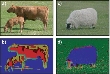
Figure 13.8 Texton maps. In a texton map each pixel is replaced by the texton index. This index characterizes the texture in the surrounding region. a) Original image. b) Associated texton map. Note how similar regions are assigned the same texton index (indicated by color). c) Original image. d) Associated texton map (using different filter bank from (b)). Texton maps are often used in semantic image segmentation. Adapted from from Shotton et al. (2009). ©2009 Springer.

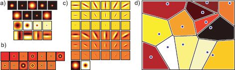
Figure 13.9 Textons. The image is convolved with a filter bank to yield an N × 1 vector of filter responses at each position. Possible choices for the filter bank include a) a combination of Gaussians, derivatives of Gaussians, and Laplacians of Gaussians; b) rotationally invariant filters; and c) the maximum response (MR8) database. d) In training, the N × 1 filter response vectors are clustered using K-means. For new data, the texton index is assigned based on the nearest of these clusters. Thus, the filter space is effectively partitioned into Voronoi regions.

13.2 Edges, corners, and interest points

In this section, we consider methods that aim to identify informative parts of the image. In edge detection the goal is to return a binary image where a nonzero value denotes the presence of an edge in the image. Edge detectors optionally also return other information such as the orientation and scale associated with the edge. Edge maps are a highly compact representation of an image, and it has been shown that it is possible to reconstruct an image very accurately with just information about the edges in the scene (Figure 13.10).

Corners are positions in the image that contain rich visual information and can be found reproducibly in different images of the same object (Figure 13.12). There are many schemes to find corners, but they all aim to identify points that are locally unique. Corner detection algorithms were originally developed for geometric computer vision problems such as wide baseline image matching; here we see the same scene from two different angles and wish to identify which points correspond to which. In recent years, corners have also been used in object recognition algorithms (where they are usually referred to as interest points). The idea here is that the regions surrounding interest points contain information about which object class is present.

13.2.1 Canny edge detector

To compute edges with the Canny edge detector (Figure 13.11), the image P is first blurred and then convolved with a pair of orthogonal derivative filters such as Prewitt filters to create images H and V containing derivatives in the horizontal and vertical directions, respectively. For pixel (i, j), the orientation θ_ij and magnitude a_ij of the gradient is computed using

A simple approach would be to assign an edge to position (i,j) if the amplitude there exceeds a critical value. This is termed thresholding. Unfortunately, it produces poor results: the amplitude map takes high values on the edge, but also at adjacent positions. The Canny edge detector eliminates these unwanted responses using a method known as non-maximum suppression.

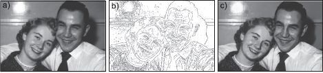
Figure 13.10 Reconstruction from edges. a) Original image. b) Edge map. Each edge pixel has associated scale and orientation information as well as a record of the luminance levels at either side. c) The image can be reconstructed almost perfectly from the edges and their associated information. Adapted from Elder (1999). ©1999 Springer.

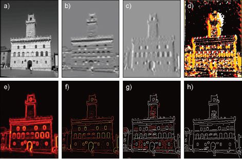
Figure 13.11 Canny edge detection. a) Original image. b) Result of vertical Prewitt filter. c) Results of horizontal Prewitt filter. d) Quantized orientation map. e) Gradient amplitude map. f) Amplitudes after non-maximum suppression. g) Thresholding at two levels: the white pixels are above the higher threshold. The red pixels are above the lower threshold but below the higher one. h) Final edge map after hysteresis thresholding contains all of the white pixels from (g) and those red pixels that connect to them.

In non-maximum suppression the gradient orientation is quantized into one of four angles {0°, 45°, 90°, 135°}, where angles 180° apart are treated as equivalent. The pixels associated with each angle are now treated separately. For each pixel, the amplitude is set to zero if either of the neighboring two pixels perpendicular to the gradient have higher values. For example, for a pixel where the gradient orientation is vertical (the image is changing in the horizontal direction), the pixels to the left and right are examined and the amplitude is set to zero if either of these are greater than the current value. In this way, the gradients at the maximum of the edge amplitude profile are retained, and those away from this maximum are suppressed.

A binary edge map can now be computed by comparing the remaining nonzero amplitudes to a fixed threshold. However, for any given threshold there will be misses (places where there are real edges, but their amplitude falls below the threshold) and false positives (pixels labeled as edges where none exist in the original image). To decrease these undesirable phenomena, knowledge about the continuity of real-world edges is exploited. Two thresholds are defined. All of the pixels whose amplitude is above the higher threshold are labeled as edges, and this threshold is chosen so that there are few false positives. To try to decrease the number of misses, pixels that are above the lower amplitude threshold and are connected to an existing edge pixel are also labeled as edges. By iterating this last step, it is possible to trace along weaker parts of strong contours. This technique is known as hysteresis thresholding.

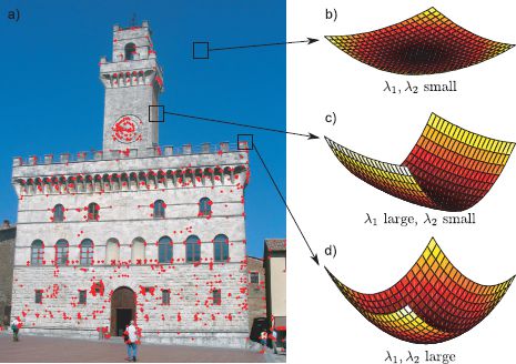
Figure 13.12 Harris corner detector. a) Image with detected corners. The corner detection algorithm is based on the image structure tensor that captures information about the distribution of gradients around the point. b) In flat regions, both singular values of the image structure tensor are small. c) On edges, one is small and the other large. d) At corners, both are large indicating that the image is changing quickly in both directions.

13.2.2 Harris corner detector

The Harris corner detector (Figure 13.12) considers the local gradients in the horizontal and vertical directions around each point. The goal is to find points in the image where the image intensity is varying in both directions (a corner) rather than in one direction (an edge) or neither (a flat region). The Harris corner detector bases this decision on the image structure tensor

where S_ij is the image structure tensor at position (i,j), which is computed over a square region of size (2D + 1) × (2D + 1) around the current position. The term h_mn denotes the response of a horizontal derivative filter (such as the Sobel) at position (m,n) and the term v_mn denotes the response of a vertical derivative filter. The term w_mn is a weight that diminishes the contribution of positions that are far from the central pixel (i,j).

To identify whether a corner is present, the Harris corner detector considers the singular values λ₁, λ₂ of the image structure tensor. If both singular values are small, then the region around the point is smooth and this position is not chosen. If one singular value is large but the other small, then the image is changing in one direction but not the other, and point lies on or near an edge. However, if both singular values are large, then this image is changing rapidly in both directions in this region and the position is deemed to be a corner.

In fact the Harris detector does not directly compute the singular values, but evaluates a criterion which accomplishes the same thing more efficiently:

where κ is a constant (values between 0.04 and 0.15 are sensible). If the value of c_ij is greater than a predetermined threshold, then a corner may be assigned. There is usually an additional non-maximum suppression stage similar to that in the Canny edge detector to ensure that only peaks in the function c_ij are retained.

13.2.3 SIFT detector

The scale invariant feature transform (SIFT) detector is a second method for identifying interest points. Unlike the Harris corner detector, it associates a scale and orientation to each of the resulting interest points. To find the interest points a number of operations are performed in turn.

The intensity image is filtered with a difference of Gaussian kernel at a series of K increasingly coarse scales (Figure 13.13). Then the filtered images are stacked to make a 3D volume of size I × J × K, where I and J are the vertical and horizontal size of the image. Extrema are identified within this volume: these are positions where the 26 3D voxel neighbors (from a 3 × 3 × 3 block) are either all greater than or all less than the current value.

These extrema are localized to subvoxel accuracy, by applying a local quadratic approximation and returning the position of the peak or trough. The quadratic approximation is made by taking a Taylor expansion about the current point. This provides a position estimate that has subpixel resolution and an estimate of the scale that is more accurate than the resolution of the scale sampling. Finally, the image structure tensor S_ij (Equation 13.14) is computed at the location and scale of each point. Candidate points in smooth regions and on edges are removed by considering the singular values of S_ij as in the Harris corner detector (Figure 13.14).

This procedure returns a set of interest points that are localized to subpixel accuracy and associated accurately with a particular scale. Finally, a unique orientation is also assigned to each interest point. To this end, the amplitude and orientation of the local gradients are computed (Equations 13.13) in a region surrounding the interest point whose size is proportional to the identified scale. An orientation histogram is then computed over this region with 36 bins covering all 360° of orientation. The contribution to the histogram depends on the gradient amplitude and is weighted by a Gaussian profile centered at the location of the interest point, so that nearby regions contribute more. The orientation of the interest point is assigned to be the peak of this histogram. If there is a second peak within 80 percent of the maximum, we may choose to compute descriptors at two orientations at this point. The final detected points are hence associated with a particular orientation and scale (Figure 13.15).

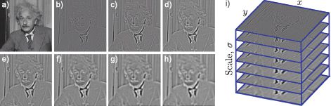
Figure 13.13 The SIFT detector. a) Original image. b-h) The image is filtered with difference of Gaussian kernels at a range of increasing scales. i) The resulting images are stacked to create a 3D volume. Points that are local extrema in the filtered image volume (i.e., are either greater than or less than all 26 3D neighbors) are considered to be candidates for interest points.

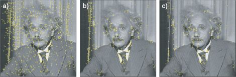
Figure 13.14 Refinement of SIFT detector candidates. a) Positions of extrema in the filtered image volume (Figure 13.13i). Note that the scale is not shown. These are considered candidates to be interest points. b) Remaining candidates after eliminating those in smooth regions. c) Remaining candidate points after removing those on edges using the image structure tensor.

13.3 Descriptors

In this section, we consider descriptors. These are compact representations that summarize the contents of an image region.

13.3.1 Histograms

The simplest approach to aggregating information over a large image region is to compute a histogram of the responses in this area. For example, we might collate RGB pixel intensities, filter responses, local binary patterns, or textons into a histogram depending on the application. The histogram entries can be treated as discrete and modeled with a categorical distribution, or treated as a continuous vector quantity.

For continuous quantities such as filter responses, the level of quantization is critical. Quantizing the responses into many bins potentially allows fine discrimination between responses. However, if data are scarce, then many of these bins will be empty, and it is harder to reliably determine the statistics of the descriptor. One approach is to use an adaptive clustering method such as K-means (Section 13.4.4) to automatically determine the bin sizes and shapes.

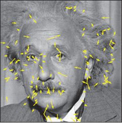
Figure 13.15 Results of SIFT detector. Each final interest point is indicated using an arrow. The length of the arrow indicates the scale with which the interest point is identified and the angle of the arrow indicates the associated orientation. Notice that there are some positions in the image where the orientation was not unique and here two interest points are used, one associated with each orientation. An example of this is on the right shirt collar. Subsequent descriptors that characterize the structure of the image around the interest points are computed relative to this scale and orientation and hence inherit some invariance to these factors.

Histogramming is a useful approach for tasks where spatial resolution is not paramount: for example, to classify a large region of texture, it makes sense to pool information. However, this approach is largely unsuitable for characterizing structured objects: the spatial layout of the object is important for identification. We now introduce two representations for image regions that retain some spatial information but also pool information locally and thus provide invariance to small displacements and warps of the image. Both the SIFT descriptor (Section 13.3.2) and the HOG descriptor (Section 13.3.3) concatenate several histograms that were computed over spatially distinct blocks.

13.3.2 SIFT descriptors

The scale invariant feature transform descriptor (Figure 13.16) characterizes the image region around a given point. It is usually used in conjunction with interest points that were found using the SIFT detector. These interest points are associated with a particular scale and rotation, and the SIFT descriptor would typically be computed over a square region that is transformed by these values. The goal is to characterize the image region in a way that is partially invariant to intensity and contrast changes and small geometric deformations.

To compute the SIFT descriptor, we first compute gradient orientation and amplitude maps (Equation 13.13) as for the Canny edge detector over a 16 × 16 pixel region around the interest point. The resulting orientation is quantized into eight bins spread over the range 0°-360°. Then the 16 × 16 detector region is divided into a regular grid of nonoverlapping 4 × 4 cells. Within each of these cells, an eight-dimensional histogram of the image orientations is computed. Each contribution to the histogram is weighted by the associated gradient amplitude and by distance so that positions further from the interest point contribute less. The 4 × 4 = 16 histograms are concatenated to make a single 128 × 8 vector, which is then normalized.

The descriptor is invariant to constant intensity changes as it is based on gradients. The final normalization provides some invariance to contrast. Small deformations do not affect the descriptor too much as it pools information within each cell. However, by keeping the information from each cell separate, some spatial information is retained.

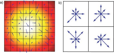
Figure 13.16 SIFT descriptor. a) Gradients are computed for every pixel within a region around the interest point. b) This region is subdivided into cells. Information is pooled within these cells to form an 8D histogram. These histograms are concatenated to provide a final descriptor that pools locally to provide invariance to small deformations but also retains some spatial information about the image gradients. In this figure, information from an 8 × 8 pixel patch has been divided to make a 2 × 2 grid of cells. In the original implementation of the SIFT detector, a 16 × 16 patch was divided into at 4 × 4 grid of cells.

13.3.3 Histogram of oriented gradients

The Histogram of Oriented Gradients (HOG) descriptor attempts to construct a more detailed characterization of the spatial structure with a small image window. It is a useful preprocessing step for algorithms that detect objects with quasi-regular structure such as pedestrians. Like the SIFT descriptor, the HOG descriptor consists of a collection of normalized histograms computed over spatially offset patches; the result is a descriptor that captures coarse spatial structure, but is invariant to small local deformations.

The process of computing a HOG descriptor suitable for pedestrian detection consists of the following stages. First, the orientation and amplitude of the image gradients are computed at every pixel in a 64 × 128 window using Equation 13.13. The orientation is quantized into nine bins spread over the range 0°-180°. The 64 × 128 detector region is divided into a regular grid of overlapping 6 × 6 cells. A 9D orientation histogram is computed within each cell, where the contribution to the histogram is weighted by the gradient amplitude and the distance from the center of the cell so that more central pixels contribute more. For each 3 × 3 block of cells, the descriptors are concatenated and normalized to form a block descriptor. All of the block descriptors are concatenated to form the final HOG descriptor.

The final descriptor contains spatially pooled information about local gradients (within each cell), but maintains some spatial resolution (as there are many cells). It creates invariance to contrast polarity by only using the gradient magnitudes. It creates invariance to local contrast strength by normalizing relative to each block. The HOG descriptor is similar in spirit to the SIFT descriptor but is distinguished by being invariant to contrast polarity, having a higher spatial resolution of computed histograms and performing normalization more locally.

13.3.4 Bag of words descriptor

The descriptors discussed thus far have been intended to characterize small regions of images. Often these regions have been connected to interest points. The bag of words representation attempts to characterize a larger region or an entire image by summarizing the statistics of the descriptors (e.g., SIFT) associated with all of the interest points in a region.

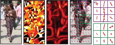
Figure 13.17 HOG descriptor. a) Original image. b) Gradient orientation, quantized into nine bins from 0° to 180°. c) Gradient magnitude. d) Cell descriptors are 9D orientation histograms that are computed within 6 × 6 pixel regions. e) Block descriptors are computed by concatenating 3 × 3 blocks of cell descriptors. The block descriptors are normalized. The final HOG descriptor consists of the concatenated block descriptors.

Each observed descriptor is considered to be one of a finite vocabulary of possible descriptors (termed visual words). Collectively, this vocabulary is known as a dictionary. The bag of words descriptor is simply a histogram describing the frequency of observing these words giving no regard to their position. To compute the dictionary, interest points are found in a large number of images and the associated descriptor is computed. These descriptors are clustered using K-means (Section 13.4.4). To compute the bag of words representation, each descriptor is assigned to the nearest word in this dictionary.

The bag of words representation is a remarkably good substrate for object recognition. This is somewhat surprising given that it surrenders any knowledge about the spatial configuration about the object. Of course, the drawback of approaches based on the bag of words is that it is very hard to localize the object after we have identified its presence or to decide how many instances are present using the same model.

13.3.5 Shape context descriptor

For certain vision tasks, the silhouette of the object contains much more information than the RGB values themselves. Consider, for example, the problem of body pose estimation: given an image of a human being, the goal is to estimate the 3D joint angles of the body. Unfortunately, the RGB values of the image depend on the person’s clothing and are relatively uninformative. In such situations, it is wiser to attempt to characterize the shape of the object.

The shape context descriptor is a fixed length vector that characterizes the object contour. Essentially, it encodes the relative position of points on the contour. In common with the SIFT and HOG descriptors, it pools information locally over space to provide a representation that can capture the overall structure of the object but is not affected too much by small spatial variations.

To compute the shape context descriptor (Figure 13.18), a discrete set of points is sampled along the contour of the object. A fixed length vector is associated with each point that characterizes the relative position of the other points. To this end, a log polar sampling array is centered on the current point. A histogram is then computed where each bin contains the number of the other points on the silhouette that fell into each bin of the log-polar array. The choice of the log-polar scheme means that the descriptor is very sensitive to local changes in the shape, but only captures the approximate configuration of distant parts.

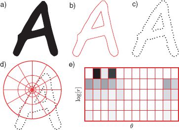
Figure 13.18 Shape context descriptor. a) Object silhouette. b) Contour of silhouette. c) Points are placed at equally spaced intervals around the silhouette. d) A log polar sampling array is centered at each point. e) The shape of the object relative to this point is captured by the histogram over the bins of the log polar array. The final descriptor would consist of a concatenation of the values from histograms from multiple points around the edge of the object.

The collection of histograms for all of the points on this image captures the shape. However, to directly match to another shape, the point correspondence must be established. It is possible to make this descriptor invariant to orientation by evaluating the orientation of the contour at each point and rotating the log polar sampling scheme so that it is aligned with this orientation.

13.4 Dimensionality reduction

It is often desirable to reduce the dimensionality of either the original or pre-processed image data. If we can do this without losing too much information, then the resulting models will require fewer parameters and be faster to learn and to use for inference.

Dimensionality reduction is possible because a given type of image data (e.g., RGB values from face images) usually lie in a tiny subset of the possible data space; not all sets of RGB values look like real images, and not all real images look like faces. We refer to the subset of the space occupied by a given dataset as a manifold. Dimensionality reduction can hence be thought of as a change of variables: we move from the original coordinate system to the (reduced) coordinate system within the manifold.

Our goal is hence to find a low-dimensional (or hidden) representation h, which can approximately explain the data x, so that

where f[•,•] is a function that takes the hidden variable and a set of parameters θ. We would like the lower-dimensional representation to capture all of the relevant variation in the original data. Hence, one possible criterion for choosing the parameters is to minimize the least squares reconstruction error so that

where x_i is the i^th of I training examples. In other words, we aim to find a set of low-dimensional variables {h_i}^I_i=1 and a mapping from h to x so that it reconstructs the original data as closely as possible in a least squares sense.

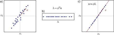
Figure 13.19 Reduction to a single dimension. a) Original data and direction of maximum variance. b) The data are projected onto to produce a one-dimensional representation. c) To reconstruct the data, we remultiply by . Most of the original variation is retained. PCA extends this model to project high-dimensional data onto the K orthogonal dimensions with the most variance, to produce a K-dimensional representation.

13.4.1 Approximation with a single number

Let us first consider a very simple model in which we attempt to represent each observed datum with a single number (Figure 13.19) so that

where the parameter μ is the mean of the data is zero and the parameter is a basis vector mapping the low-dimensional representation h back to the original data space x. For simplicity, we will assume from now on that the mean of the x_i ≈ h_i. This can be achieved by computing the empirical mean μ and subtracting it from every example x_i.

The learning algorithm optimizes the criterion

Careful consideration of the cost function (Equation 13.19) reveals an immediate problem: the solution is ambiguous as we can multiply the basis function by any constant K and divide each of the hidden variables {h_i}^I_i=1 by the same number to yield exactly the same cost. To resolve this problem, we force the vector to have unit length. This is accomplished by adding in a Lagrange multiplier λ so that the cost function becomes

To minimize the function, we first take the derivative with respect to h_i and then equate the resulting expression to zero to yield

In other words, to find the reduced dimension representation h_i we simply project the observed data onto the vector .

We now take the derivative of Equation 13.20 with respect to , substitute in the solution for h_i, equate the result to zero, and rearrange to get

or in matrix form

where the matrix X = [x₁, x₂,…, x_I] contains the data examples in its columns. This is an eigenvalue problem. To find the optimal vector, we compute the SVD ULV^T = XX^T and choose the first column of U.

The scatter matrix XX^T is a constant multiple of the covariance matrix, and so this has a simple geometric interpretation. The optimal vector to project onto corresponds to the principal direction of the covariance ellipse. This makes intuitive sense; we retain information from the direction in space where the data vary most.

13.4.2 Principal component analysis

Principal component analysis (PCA) generalizes the above model. Instead of finding a scalar variable h_i that represents the i^th data example x_i, we now seek a K-dimensional vector h_i. The relation between the hidden and observed spaces is

where the matrix Φ = [₁,₂,…,_K] contains K basis functions or principal components; the observed data are modeled as a weighted sum of the principal components, where the k^th dimension of h_i weights the k^th component.

The solution for the unknowns Φ and h_1…I can now be written as

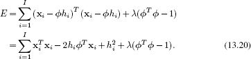
Once more, the solution to this is nonunique as we can postmultiply Φ by any matrix A and premultiply each hidden variable h_i by the inverse A⁻¹ and still get the same cost. To (partially) resolve this problem, we add the extra constraint that Φ^T Φ = I. In other words, we force the principal components to be orthogonal and length one. This gives a modified cost function of

where λ is a Lagrange multiplier. We now minimize this expression with respect to Φ, h_1…I and λ. The expression for the hidden variables becomes

The K principal components Φ = [₁,₂,…,_K] are now found by computing the singular value decomposition ULV^T = XX^T and taking the first K columns of U. In other words, to reduce the dimensionality, we project the data x_ionto a hyperplane defined by the K largest axes of the covariance ellipsoid.

This algorithm is very closely related to probabilistic principal component analysis (Section 17.5.1). Probabilistic PCA additionally models the noise that accounts for the inexact approximation in Equation 13.24. Factor analysis (Section 7.6) is also very similar, but constructs a more sophisticated model of this noise.

13.4.3 Dual principal component analysis

The method outlined in Section 13.4.2 requires us to compute the SVD of the scatter matrix XX^T. Unfortunately, if the data had dimension D, then this is a D × D matrix, which may be very large. We can sidestep this problem by using dual variables. We define Φ as a weighted sum of the original datapoints so that

where Ψ = [ψ₁,ψ₂,…,ψ_K] is a I × K matrix representing these weights. The associated cost function now becomes

The solution for the hidden variables becomes

and the K dual principal components Ψ = [ψ₁,ψ₂…, ψ_K] are extracted from the matrix U in the SVD ULV^T = X^TX. This is a smaller problem of size I × I and so is more efficient when the number of data examples I is less than the dimensionality of the observed space D.

Notice that this algorithm does not require the original datapoints: it only requires the inner products between them and so it is amenable to kernelization. This resulting method is known as kernel PCA.

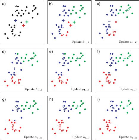
Figure 13.20 K-means algorithm for K = 3 clusters. a) We initialize the three prototype vectors (crosses) to random positions. We alternately b) assign the data to the nearest prototype vector and c) update the prototype vectors to be equal to the mean of the points assigned to them. d-i) We repeat these steps until there is no further change.

13.4.4 The K-means algorithm

A second common approach to dimensionality reduction is to abandon a continuous representation altogether and represent the each datapoint using one of a limited set of prototype vectors. In this model, the data are approximated as

where h_i ∈ {1,2,…, K} is an index that identifies which of the K prototype vectors {μ_k}^K_k=1 approximates the i^th example.

To find the assignment indices and the prototype vectors (Figure 13.20), we optimize

In the K-means algorithm, this cost function is minimized using an alternating strategy in which we first assign each datapoint to the nearest prototype

and then update the prototypes

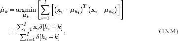
where δ[•] is a function that returns one when its argument is zero and zero otherwise. In other words, the new prototype is simply the average of the datapoints that are assigned to this cluster. This algorithm is not guaranteed to converge to the global minimum and so it requires sensible starting conditions.

The K-means algorithm is very closely related to the mixtures of Gaussians model (Section 7.4). The main differences are that the mixtures of Gaussians model is probabilistic and defines a density over the data space. It also assigns weights to the clusters and describes their covariance.

Conclusion

Careful reading of the information in this chapter should convince you that there are certain recurring ideas in image preprocessing. To make a descriptor invariant to intensity changes we filter the image and normalize the filter responses over the region. A unique descriptor orientation and scale can be computed by maximizing over responses at different orientations and scales. To create invariance to small spatial changes, local responses are pooled. Despite the simplicity of these ideas, it is remarkable how much impact they have on the performance of real systems.

Notes

Image Processing: There are numerous texts on image processing which contain far more information than I could include in this chapter. I would particularly recommend the books by O’Gorman et al. (2008), Gonzalez and Woods (2002), Pratt (2007), and Nixon and Aguado (2008). A comprehensive recent summary of local image features can be found in Li and Allinson (2008).

Edge and corner detection: The Canny edge detector was first described in Canny (1986). Elder (1999) investigated whether it was possible to reconstruct an image based on edge information alone. Nowadays, it is common to use machine learning methods to identify object boundaries in images (e.g., Dollár et al. 2006)

Early work in corner detection (interest point detection) includes that of Moravec (1983), Förstner (1986), and the Harris corner detector (Harris and Stephens 1988), which we described in this chapter. Other more recent efforts to identify stable points and regions include the SUSAN corner detector (Smith and Brady 1997), a saliency-based descriptor (Kadir and Brady 2001), maximally stable extremal regions (Matas et al. 2002), the SIFT detector (Lowe 2004), and the FAST detector (Rosten and Drummond 2006). There has been considerable recent interest in affine invariant interest point detection, which aims to find features that are stable under affine transformations of the image (e.g., Schaffalitzky and Zisserman 2002; Mikolajczyk and Schmid 2002, 2004). Mikolajczyk et al. (2005) present a quantitative comparison of different affine region detectors. A recent review of this area can be found in Tuytelaars and Mikolajczyk (2007).

Image descriptors: For robust object recognition and image matching, it is crucial to characterize the region around the detected interest point in a way that is compact and stable to changes in the image. To this end, Lowe (2004) developed the SIFT descriptor, Dalal and Triggs (2005) developed the HOG descriptor, and Forssén and Lowe (2007) developed a descriptor for use with maximally stable extremal regions. Bay et al. (2008) developed a very efficient version of SIFT features known as SURF. Mikolajczyk and Schmid (2005) present a quantitative comparison of region descriptors. Recent work on image descriptors has applied machine learning techniques to optimize their performance (Brown et al. 2011; Philbin et al. 2010).

More information about local binary patterns can be found in Ojala et al. (2002). More information about the shape context descriptor can be found in Belongie et al. (2002).

Dimensionality reduction: Principal components analysis is a linear dimensionality reduction method. However, there are also many nonlinear approaches that describe a manifold of images in high dimensions with fewer parameters. Notable methods include kernel PCA (Scholköpf et al. 1997), ISOMAP (Tenenbaum et al. 2000), local linear embedding (Roweis and Saul 2000), charting (Brand 2002), the Gaussian process latent variable model (Lawrence 2004), and Laplacian eigenmaps (Belkin and Niyogi 2001). Recent reviews of dimensionality reduction can be found in Burgess (2010) and De La Torre (2011).

Problems

13.1 Consider an eight-bit image in which the pixel values are evenly distributed in the range 0-127, with no pixels taking a value of 128 or larger. Draw the cumulative histogram for this image (see Figure 13.2). What will the histogram of pixel intensities look like after applying histogram equalization?

13.2 Consider a continuous image p[i,j] and a continuous filter f[n,m] In the continuous domain, the operation f ⊗ p of convolving an image with the filter is defined as

Now consider two filters f and g. Prove that convolving the image first with f and then with g has the same effect as convolving f with g and then convolving the image with the result. In other words:

Does this result extend to discrete images?

13.3 Describe the series of operations that would be required to compute the Haar filters in Figures 13.6a-d from an integral image. How many points from the integral image are needed to compute each?

13.4 Consider a blurring filter where each pixel in an image is replaced by a weighted average of local intensity values, but the the weights decrease if these intensity values differ markedly from the central pixel. What effect would this bilateral filter have when applied to an image?

13.5 Define a 3 × 3 filter that is specialized to detecting luminance changes at a 45^o angle and gives a positive response where the image intensity increases from the bottom left to the bottom right of the image.

13.6 Define a 3 × 3 filter that responds to the second derivative in the horizontal direction but is invariant to the gradient and absolute intensity in the horizontal direction and invariant to all changes in the vertical direction.

13.7 Why are most local binary patterns in a natural image typically uniform or near-uniform?

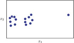
Figure 13.21 Clustering with the K-means algorithm in the presence of outliers (Problem 13.9). This data set contains two clusters and a single outlier (the point on the right-hand side). The outlier causes problems for the K-means algorithm when K = 2 clusters are used due to the implicit assumption that the clusters can be modeled as normal distributions with spherical covariance.

13.8 Give one example of a 2D data set where the mixtures of Gaussians model will succeed in clustering the data, but the K-means algorithm will fail.

13.9 Consider the data in Figure 13.21. What do you expect to happen if we run the K-means algorithm on this data set? Suggest a way to resolve this problem.

13.10 An alternative approach to clustering the data would be to find modes (peaks) in the density of the points. This potentially has the advantage of also automatically selecting the number of clusters. Propose an algorithm to find these modes.