Computer Vision: Models, Learning, and Inference (2012)
Part V
Models for geometry
In Part V, we finally acknowledge the process by which real-world images are formed. Light is emitted from one or more sources and travels through the scene, interacting with the materials via physical processes such as reflection, refraction, and scattering. Some of this light enters the camera and is measured. We have a very good understanding of this forward model. Given known geometry, light sources, and material properties, computer graphics techniques can simulate what will be seen by the camera very accurately.
The ultimate goal for a vision algorithm would be a complete reconstruction, in which we aim to invert this forward model and estimate the light sources, materials, and geometry from the image. Here, we aim to capture a structural description of the world: we seek an understanding of where things are and to measure their optical properties, rather than a semantic understanding. Such a structural description can be exploited to navigate around the environment or build 3D models for computer graphics.
Unfortunately, full visual reconstruction is very challenging. For one thing, the solution is nonunique. For example, if the light source intensity increases, but the object reflectance decreases commensurately, the image will remain unchanged. Of course, we could make the problem unique by imposing prior knowledge, but even then reconstruction remains difficult; it is hard to effectively parameterize the scene, and the problem is highly non-convex.
In this part of the book, we consider a family of models that approximate both the 3D scene and the observed image with sparse sets of visual primitives (points). The forward model that maps the proxy representation of the world (3D points) to the proxy representation of the image (2D points) is much simpler than the full light transport model, and is called the projective pinhole camera. We investigate the properties of this model in Chapter 14.
In Chapter 15, we consider the situation where the pinhole camera views a plane in the world; there is now a one-to-one mapping between points on the plane and points in the image, and we characterize this mapping with a family of 2D transformations. In Chapter 16, we will further exploit the pinhole camera model to recover a sparse geometric model of the scene.
Chapter 14
The pinhole camera
This chapter introduces the pinhole or projective camera. This is a purely geometric model that describes the process whereby points in the world are projected into the image. Clearly, the position in the image depends on the position in the world, and the pinhole camera model captures this relationship.
To motivate this model, we will consider the problem of sparse stereo reconstruction (Figure 14.1). We are given two images of a rigid object taken from different positions. Let us assume that we can identify corresponding 2D features between the two images - points that are projected versions of the same position in the 3D world. The goal now is to establish this 3D position using the observed 2D feature points. The resulting 3D information could be used by a robot to help it navigate through the scene, or to facilitate object recognition.
14.1 The pinhole camera
In real life, a pinhole camera consists of a chamber1 with a small hole (the pinhole) in the front (Figure 14.2). Rays from an object in the world pass through this hole to form an inverted image on the back face of the box, or image plane. Our goal is to build a mathematical model of this process.
It is slightly inconvenient that the image from the pinhole camera is upside-down. Hence, we instead consider the virtual image that would result from placing the image plane in front of the pinhole. Of course, it is not physically possible to build a camera this way, but it is mathematically equivalent to the true pinhole model (except that the image is the right way up) and it is easier to think about. From now on, we will always draw the image plane in front of the pinhole.
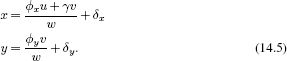
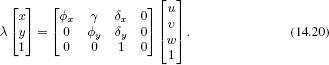
Figure 14.3 illustrates the pinhole camera model and defines some terminology. The pinhole itself (the point at which the rays converge) is called the optical center. We will assume for now that the optical center is at the origin of the 3D world coordinate system, in which points are represented as w = [u,v,w]T. The virtual image is created on the image plane, which is displaced from the optical center along the w-axis or optical axis. The point where the optical axis strikes the image plane is known as the principal point. The distance between the principal point and the optical center (i.e., the distance between the image plane and the pinhole) is known as the focal length.
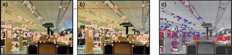
Figure 14.1 Sparse stereo reconstruction. a,b) We are given two images of the same scene taken from different positions, and a set of I pairs of points in these images that are known to correspond to the same points in the world (e.g., the points connected by the red line are a corresponding pair). c) Our goal is to establish the 3D position of each of the world points. Here, the depth is encoded by color so that closer points are red and more distant points are blue.
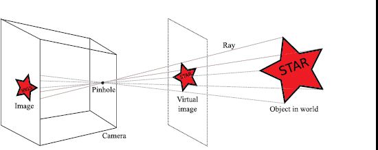
Figure 14.2 The pinhole camera model. Rays from an object in the world pass through the pinhole in the front of the camera and form an image on the back plane (the image plane). This image is upside-down, so we can alternatively consider the virtual image that would have been created if the image plane was in front of the pinhole. This is not physically possible, but it is more convenient to work with.
The pinhole camera model is a generative model that describes the likelihood Pr(x|w) of observing a feature at position x = [x,y]T in the image given that it is the projection of a 3D point w = [u,v,w]T in the world. Although light transport is essentially deterministic, we will nonetheless build a probability model; there is noise in the sensor, and unmodeled factors in the feature detection process can also affect the measured image position. However, for pedagogical reasons we will defer a discussion of this uncertainty until later, and temporarily treat the imaging process as if it were deterministic.
Our task then is to establish the position x = [x,y]T where the 3D point w = [u,v,w]T is imaged. Considering Figure 14.3 it is clear how to do this. We connect a ray between w and the optical center. The image position x can be found by observing where this ray strikes the image plane. This process is called perspective projection. In the next few sections, we will build a more precise mathematical model of this process. We will start with a very simple camera model (the normalized camera) and build up to a full camera parameterization.
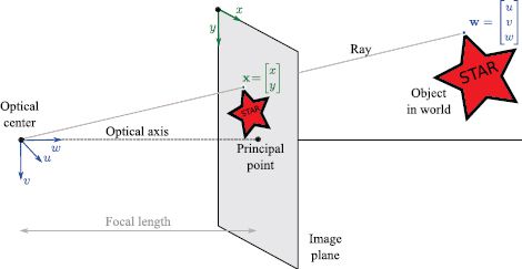
Figure 14.3 Pin-hole camera model terminology. The optical center (pinhole) is placed at the origin of the 3D world coordinate system (u,v,w) and the image plane (where the virtual image is formed) is displaced along the w-axis, which is also known as the optical axis. The position where the optical axis strikes the image plane is called the principal point. The distance between the image plane and the optical center is called the focal length.
14.1.1 The normalized camera
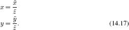
In the normalized camera, the focal length is one, and it is assumed that the origin of the 2D coordinate system (x,y) on the image plane is centered at the principal point. Figure 14.4 shows a 2D slice of the geometry of this system (the u- and x-axes now point upward out of the page and cannot be seen). By similar triangles, it can easily be seen that the y-position in the image of the world point at w = [u, v, w]T is given by v/w. More generally, in the normalized camera, a 3D point w = [u, v, w]T is projected into the image at x = [x,y]T using the relations
where x,y,u,v, and w are measured in the same real-world units (e.g., mm).
14.1.2 Focal length parameters
The normalized camera is unrealistic; for one thing, in a real camera, there is no particular reason why the focal length should be one. Moreover, the final position in the image is measured in pixels, not physical distance, and so the model must take into account the photoreceptor spacing. Both of these factors have the effect of changing the mapping between points w = [u,v,w]T in the 3D world and their 2D positions x = [x,y]T in the image plane by a constant scaling factor ![]() (Figure 14.5) so that
(Figure 14.5) so that
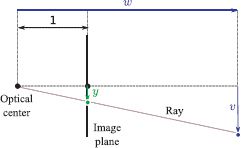
Figure 14.4 Normalized camera. The focal length is one, and the 2D image coordinate system (x, y) is centered on the principal point (only y-axis shown). By similar triangles, the y position in the image of a point at (u,v,w) is given by v/w. This corresponds to our intuition: as an object gets more distant, its projection becomes closer to the center of the image.
To add a further complication, the spacing of the photoreceptors may differ in the x- and y-directions, so the scaling may be different in each direction, giving the relations
where ![]() x and
x and ![]() y are separate scaling factors for the x- and y-directions. These parameters are known as the focal length parameters in the x- and y-directions, but this name is somewhat misleading - they account for not just the distance between the optical center and the principal point (the true focal length) but also the photoreceptor spacing.
y are separate scaling factors for the x- and y-directions. These parameters are known as the focal length parameters in the x- and y-directions, but this name is somewhat misleading - they account for not just the distance between the optical center and the principal point (the true focal length) but also the photoreceptor spacing.
14.1.3 Offset and skew parameters
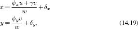
The model so far is still incomplete in that pixel position x = [0,0]T is at the principal point (where the w-axis intersects the image plane). In most imaging systems, the pixel position x = [0,0]T is at the top-left of the image rather than the center. To cope with this, we add offset parameters δx and δy so that
where δx and δy are the offsets in pixels from the top-left corner of the image to the position where the w-axis strikes the image plane. Another way to think about this is that the vector [δx, δy]T is the position of the principal point in pixels.
If the image plane is exactly centered on the w-axis, these offset parameters should be half the image size: for a 640 × 480 VGA image δx and δy would be 320 and 240, respectively. However, in practice it is difficult and superfluous to manufacture cameras with the imaging sensor perfectly centered, and so we treat the offset parameters as unknown quantities.
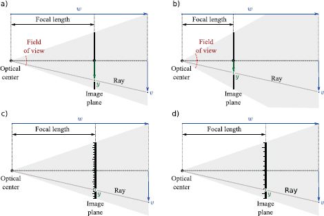
Figure 14.5 Focal length and photoreceptor spacing. a-b) Changing the distance between the optical center and the image plane (the focal length) changes the relationship between the 3D world point w = [u,v,w]T and the 2D image point x = [x,y]T. In particular, if we take the original focal length (a) and halve it (b), the 2D image coordinate is also halved. The field of view of the camera is the total angular range that is imaged (usually different in the x- and y-directions). When the focal length decreases, the field of view increases. c-d) The position in the image x = [x,y]T is usually measured in pixels. Hence, the position x depends on the density of the receptors on the image plane. If we take the original photoreceptor density (c) and halve it (d), then the 2D image coordinate is also halved. Hence, the photoreceptor spacing and focal length both change the mapping from rays to pixels in the same way.
We also introduce a skew term γ that moderates the projected position x as a function of the height v in the world. This parameter has no clear physical interpretation but can help explain the projection of points into the image in practice. The resulting camera model is
14.1.4 Position and orientation of camera
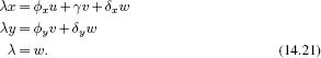
Finally, we must account for the fact that the camera is not always conveniently centered at the origin of the world coordinate system with the optical axis exactly aligned with the w-axis. In general, we may want to define an arbitrary world coordinate system that may be common to more than one camera. To this end, we express the world points w in the coordinate system of the camera before they are passed through the projection model, using the coordinate transformation:
![]()
or
![]()
where w′ is the transformed point, Ω is a 3 × 3 rotation matrix, and τ is a 3× 1 translation vector.
14.1.5 Full pinhole camera model
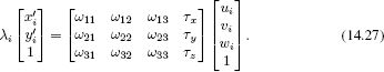
We are now in a position to describe the full camera model, by combining Equations 14.5 and 14.6. A 3D point w = [u,v,w]T is projected to a 2D point x = [x, y]T by the relations
There are two sets of parameters in this model. The intrinsic or camera parameters {![]() x,
x, ![]() y, γ, δx, δy} describe the camera itself, and the extrinsic parameters {Ω, τ} describe the position and orientation of the camera in the world. For reasons that will become clear in Section 14.3.1, we will store the intrinsic parameters in the intrinsic matrix Λ where
y, γ, δx, δy} describe the camera itself, and the extrinsic parameters {Ω, τ} describe the position and orientation of the camera in the world. For reasons that will become clear in Section 14.3.1, we will store the intrinsic parameters in the intrinsic matrix Λ where
![]()
We can now abbreviate the full projection model (Equations 14.8) by just writing
![]()
Finally, we must account for the fact that the estimated position of a feature in the image may differ from our predictions. There are a number of reasons for this, including noise in the sensor, sampling issues, and the fact that the detected position in the image may change at different viewpoints. We model these factors with additive noise that is normally distributed with a spherical covariance to give the final relation
![]()
where σ2 is the variance of the noise.
Note that the pinhole camera is a generative model. We are describing the likelihood Pr(x|w, Λ, Ω, τ) of observing a 2D image point x given the 3D world point w and the parameters {Λ, Ω, τ}.
Figure 14.6 Radial distortion. The pinhole model is only an approximation of the true imaging process. One important deviation from this model is a 2D warping in which points deviate from their expected positions by moving along radial lines from the center of the image by an amount that depends on the distance from the center. This is known as radial distortion. a) An image that suffers from radial distortion is easily spotted because lines that were straight in the world are mapped to curves in the image (e.g., red dotted line). b) After applying the inverse radial distortion model, straight lines in the world now correctly map to straight lines in the image. The distortion caused the magenta point to move along the red radial line to the position of the yellow point.
14.1.6 Radial distortion
In the previous section, we introduced the pinhole camera model. However, it has probably not escaped your attention that real-world cameras are rarely based on the pinhole: they have a lens (or possibly a system of several lenses) that collects light from a larger area and refocuses it on the image plane. In practice, this leads to a number of deviations from the pinhole model. For example, some parts of the image may be out of focus, which essentially means that the assumption that a point in the world w maps to a single point in the image x is no longer valid. There are more complex mathematical models for cameras that deal effectively with this situation, but they are not discussed here.
However, there is one deviation from the pinhole model that must be addressed. Radial distortion is a nonlinear warping of the image that depends on the distance from the center of the image. In practice, this occurs when the field of view of the lens system is large. It can easily be detected in an image because straight lines in the world no longer project to straight lines in the image (Figure 14.6).
Radial distortion is commonly modeled as a polynomial function of the distance r from the center of the image. In the normalized camera, the final image positions (x′,y′) are expressed as functions of the original positions (x,y) by
![]()
where the parameters β1 and β2 control the degree of distortion. These relations describe a family of possible distortions that approximate the true distortion closely for most common lenses.
This distortion is implemented after perspective projection (division by w) but before the effect of the intrinsic parameters (focal length, offset, etc.), so the warping is relative to the optical axis and not the origin of the pixel coordinate system. We will not discuss radial distortion further in this volume. However, it is important to realize that for accurate results, all of the algorithms in this and Chapters 15 and 16 should account for radial distortion. When the field of view is large, it is particularly critical to incorporate this into the pinhole camera model.
14.2 Three geometric problems
Now that we have described the pinhole camera model, we will consider three important geometric problems. Each is an instance of learning or inference within this model. We will first describe the problems themselves, and then tackle them one by one later in the chapter.
14.2.1 Problem 1: Learning extrinsic parameters
We aim to recover the position and orientation of the camera relative to a known scene. This is sometimes known as the perspective-n-point (PnP) problem or the exterior orientation problem. One common application is augmented reality, where we need to know this relationship to render virtual objects that appear to be stable parts of the real scene.
The problem can be stated more formally as follows: we are given a known object, with I distinct 3D points {wi}Ii=1, their corresponding projections in the image {xi}Ii=1, and known intrinsic parameters Λ. Our goal is to estimate the rotation Ω and translation τ that map points in the coordinate system of the object to points in the coordinate system of the camera so that
![]()
This is a maximum likelihood learning problem, in which we aim to find parameters Ω, τ that make the predictions pinhole[wi, Λ, Ω, τ] of the model agree with the observed 2D points xi (Figure 14.7).
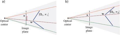
Figure 14.7 Problem 1 - Learning extrinsic parameters (exterior orientation problem). Given points {wi}Ii=1 on a known object (blue lines), their positions {xi}Ii=1 in the image (circles on image plane), and known intrinsic parameters Λ, find the rotation Ω and translation τ relating the camera and the object. a) When the rotation or translation are wrong, the image points predicted by the model (where the rays strike the image plane) do not agree well with the observed points xi. b) When the rotation and translation are correct, they agree well and the likelihood Pr(xi|w, Λ, Ω, τ) will be high.
14.2.2 Problem 2: Learning intrinsic parameters
We aim to estimate the intrinsic parameters Λ that relate the direction of rays through the optical center to coordinates on the image plane. This estimation process is known as calibration. Knowledge of the intrinsic parameters is critical if we want to use the camera to build 3D models of the world.
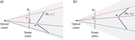
Figure 14.8 Problem 2 - Learning intrinsic parameters. Given a set of points {wi}Ii=1 on a known object in the world (blue lines) and the 2D positions {x}Ii=1 of these points in an image, find the intrinsic parameters Λ. To do this, we must also simultaneously estimate the extrinsic parameters Ω, τ. a) When the intrinsic or extrinsic parameters are wrong, the prediction of the pinhole camera (where rays strike the image plane) will deviate significantly from the observed 2D points. b) When the intrinsic and extrinsic parameters are correct, the prediction of the model will agree with the observed image.
The calibration problem can be stated more formally as follows: given a known 3D object, with I distinct 3D points {wi}Ii=1 and their corresponding projections in the image {xi}Ii=1, estimate the intrinsic parameters:
![]()
Once more this is a maximum likelihood learning problem in which we aim to find parameters Λ, Ω, τ that make the predictions of the model pinhole[wi, Λ, Ω, τ] agree with the observed 2D points xi (Figure 14.8). We do not particularly care about the extrinsic parameters Ω, τ; finding these is just a means to the end of estimating the intrinsic parameters Λ.
The calibration process requires a known 3D object, on which distinct points can be identified, and their corresponding projections in the image found. A common approach is to construct a bespoke 3D calibration target2 that achieves these goals (Figure 14.9).
14.2.3 Problem 3: Inferring 3D world points
We aim to estimate the 3D position of a point w in the scene, given its projections {xj}Jj=1 in J ≥ 2 calibrated cameras. When J = 2, this is known as calibrated stereo reconstruction. With J > 2 calibrated cameras, it is known to as multiview reconstruction. If we repeat this process for many points, the result is a sparse 3D point cloud. This could be used to help an autonomous vehicle navigate through the environment or to generate an image of the scene from a new viewpoint.
More formally, the multiview reconstruction problem can be stated as follows: given J calibrated cameras in known positions (i.e., cameras with known Λ, Ω, τ) viewing the same 3D point w and knowing the corresponding 2D projections {xj}Jj=1, in the J images establish the 3D position w of the point in the world:
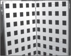
Figure 14.9 Camera calibration target. One way to calibrate the camera (estimate its intrinsic parameters) is to view a 3D object (a camera calibration target) for which the geometry is known. The marks on the surface are at known 3D positions in the frame of reference of the object and are easy to locate in the image using basic image-processing techniques. It is now possible to find the intrinsic and extrinsic parameters that optimally map the known 3D positions to their 2D projections in the image. Image from Hartley and Zisserman (2004).
![]()
The form of this inference problem is similar to that of the preceding learning problems: we perform an optimization in which we manipulate the variable of interest w until the predictions pinhole[w, Λj, Ωj, τj] of the pinhole camera models agree with the data xj (Figure 14.10). For obvious reasons, the principle behind reconstruction is known as triangulation.
14.2.4 Solving the problems
We have introduced three geometric problems, each of which took the form of a learning or inference problem using the pinhole camera model. We formulated each in terms of maximum likelihood estimation, and in each case this results in an optimization problem.
Unfortunately, none of the resulting objective functions can be optimized in closed form; each solution requires the use of nonlinear optimization. In each case, it is critical to have a good initial estimate of the unknown quantities to ensure that the optimization process converges to the global maximum. In the remaining part of this chapter, we develop algorithms that provide these initial estimates. The general approach is to choose new objective functions that can be optimized in closed form, and where the solution is close to the solution of the true problem.
14.3 Homogeneous coordinates
To get good initial estimates of the geometric quantities in the preceding optimization problems, we play a simple trick: we change the representation of both the 2D image points and 3D world points so that the projection equations become linear. After this change, it is possible to find solutions for the unknown quantities in closed form. However, it should be emphasized that these solutions do not directly address the original optimization criteria: they minimize more abstract objective functions based on algebraic error whose solutions are not guaranteed to be the same as those for the original problem. However, they are generally close enough to provide a good starting point for a nonlinear optimization of the true cost function.
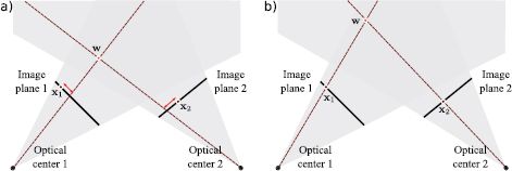
Figure 14.10 Problem 3 - Inferring 3D world points. Given two cameras with known position and orientation, and the projections x1 and x2 of the same 3D point in each image, the goal of calibrated stereo reconstruction is to infer the 3D position w of the world point. a) When the estimate of the world point (red circle) is wrong, the predictions of the pinhole camera model (where rays strike the image plane) will deviate from the observed data (brown circles on image plane). b) When the estimate of w is correct, the predictions of the model agree with the observed data.
We convert the original Cartesian representation of the 2D image points x to a 3D homogeneous coordinate ![]() so that
so that
![]()
where λ is an arbitrary scaling factor. This is a redundant representation in that any scalar multiple λ represents the same 2D point. For example, the homogeneous vectors ![]() =[2,4,2]T and
=[2,4,2]T and ![]() = [3,6,3]T both represent the Cartesian 2D point x = [1,2]T, where scaling factors λ = 2 and λ = 3 have been used, respectively.
= [3,6,3]T both represent the Cartesian 2D point x = [1,2]T, where scaling factors λ = 2 and λ = 3 have been used, respectively.
Converting between homogeneous and Cartesian coordinates is easy. To move to homogeneous coordinates, we choose λ = 1 and simply append a 1 to the original 2D Cartesian coordinate. To recover the Cartesian coordinates, we divide the first two entries of the homogeneous 3-vector by the third, so that if we observe the homogeneous vector ![]() =[
=[![]() ,
, ![]() ,
, ![]() ]T, then we can recover the Cartesian coordinate x = [x,y]T as
]T, then we can recover the Cartesian coordinate x = [x,y]T as
Further insight into the relationship between the two representations is given in Figure 14.11.
It is similarly possible to represent the 3D world point w as a homogenous 4D vector ![]() so that
so that
where λ is again an arbitrary scaling factor. Once more, the conversion from Cartesian to homogeneous coordinates can be achieved by appending a 1 to the original 3D vector w. The conversion from homogeneous to Cartesian coordinates is achieved by dividing each of the first three entries by the last.
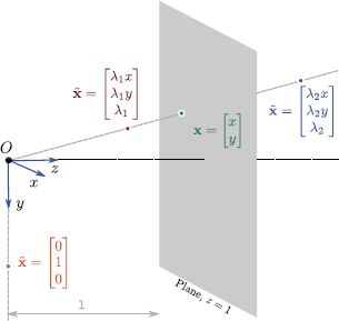
Figure 14.11 Geometric interpretation of homogeneous coordinates. The different scalar multiples λ of the homogeneous 3-vector ![]() define a ray through the origin of a coordinate space. The corresponding 2D image point x can be found by considering the 2D point that this ray strikes on the plane z = 1. An interesting side-effect of this representation is that it is possible to represent points at infinity (known as ideal points). For example, the homogeneous coordinate [0,1,0]T defines a ray that is parallel to z = 1 and so never intersects the plane. It represents the point at infinity in direction [0,1]T.
define a ray through the origin of a coordinate space. The corresponding 2D image point x can be found by considering the 2D point that this ray strikes on the plane z = 1. An interesting side-effect of this representation is that it is possible to represent points at infinity (known as ideal points). For example, the homogeneous coordinate [0,1,0]T defines a ray that is parallel to z = 1 and so never intersects the plane. It represents the point at infinity in direction [0,1]T.
14.3.1 Camera model in homogeneous coordinates
It is hard to see the point of converting the 2D image points to homogeneous 3-vectors and converting the 3D world point to homogeneous 4-vectors until we reexamine the pinhole projection equations,
where we have temporarily assumed that the world point w = [u,v,w]T is in the same coordinate system as the camera.
In homogeneous coordinates, these relationships can be expressed as a set of linear equations
To convince ourselves of this, let us write these relations explicitly:
We solve for x and y by converting back to Cartesian coordinates: we divide the first two relations by the third to yield the original pinhole model (Equation 14.19).
Let us summarize what has happened: the original mapping from 3D Cartesian world points to 2D Cartesian image points is nonlinear (due to the division by w). However, the mapping from 4D homogeneous world points to 3D homogeneous image points is linear. In the homogeneous representation, the nonlinear component of the projection process (division by w) has been side-stepped: this operation still occurs, but it is in the final conversion back to 2D Cartesian coordinates, and thus does not trouble the homogeneous camera equations.
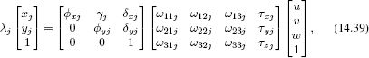
To complete the model, we add the extrinsic parameters {Ω, τ} that relate the world coordinate system and the camera coordinate system, so that
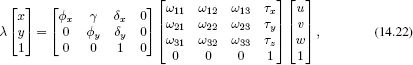
or in matrix form
![]()
where 0 = [0,0,0]T. The same relations can be simplified to
![]()
In the next three sections, we revisit the three geometric problems introduced in Section 14.2. In each case, we will use algorithms based on homogeneous coordinates to compute good initial estimates of the variable of interest. These estimates can then be improved using nonlinear optimization.
14.4 Learning extrinsic parameters
Given a known object, with I distinct 3D points {wi}Ii=1, their corresponding projections in the image {wi}Ii=1, and known intrinsic parameters Λ, estimate the geometric relationship between the camera and the object determined by the rotation Ω and the translation τ:
![]()
This is a non-convex problem, so we make progress by expressing it in homogeneous coordinates. The relationship between the ith homogeneous world point ![]() i and the ith corresponding homogeneous image point
i and the ith corresponding homogeneous image point ![]() i is
i is
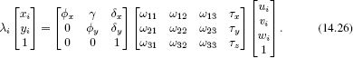
We would like to discard the effect of the (known) intrinsic parameters Λ. To this end, we premultiply both sides of the equation by the inverse of the intrinsic matrix Λ to yield
The transformed coordinates ![]() ′ = Λ−1
′ = Λ−1![]() are known as normalized image coordinates: they are the coordinates that would have resulted if we had used a normalized camera. In effect, premultiplying by Λ-1 compensates for the idiosyncrasies of this particular camera.
are known as normalized image coordinates: they are the coordinates that would have resulted if we had used a normalized camera. In effect, premultiplying by Λ-1 compensates for the idiosyncrasies of this particular camera.
We now note that the last of these three equations allows us to solve for the constant λi, so that
![]()
and we can now substitute this back into the first two equations to get the relations
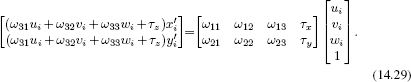
These are two linear equations with respect to the unknown quantities Ω and τ. We can take the two equations provided by each of the I pairs of points in the world w and the image x to form the system of equations
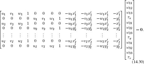
This problem is now in the standard form Ab = 0 of a minimum direction problem. We seek the value of b that minimizes |Ab|2 subject to the constraint |b| = 1 (to avoid the uninteresting solution b = 0). The solution can be found by computing the singular value decomposition A = ULVT and setting ![]() to be the last column of V (see Appendix C.7.2).
to be the last column of V (see Appendix C.7.2).
The estimates of Ω and τ that we extract from b have had an arbitrary scale imposed on them, and we must find the correct scaling factor. This is possible because the rotation Ω has a predefined scale (its rows and columns must all have norm one). In practice, we first find the closest true rotation matrix to Ω, which also forces our estimate to be a valid orthogonal matrix. This is an instance of the orthogonal Procrustes problem (Appendix C.7.3). The solution is found by computing the singular value decomposition Ω = ULVT and setting ![]() = UVT. Now, we rescale the translation τ. The scaling factor can be estimated by taking the average ratio of the nine entries of our initial estimate of Ω to the final one,
= UVT. Now, we rescale the translation τ. The scaling factor can be estimated by taking the average ratio of the nine entries of our initial estimate of Ω to the final one, ![]() so that
so that
![]()
Finally, we must check that the sign of τz is positive, indicating that the object is in front of the camera. If this is not the case, then we multiply both ![]() and
and ![]() by minus 1.
by minus 1.
This scrappy algorithm is typical of methods that use homogeneous coordinates. The resulting estimates ![]() and
and ![]() can be quite inaccurate in the presence of noise in the measured image positions. However, they usually suffice as a reasonable starting point for the subsequent nonlinear optimization of the true objective function (Equation 14.25) for this problem. This optimization must be carried out while ensuring that Ω remains a valid rotation matrix (see Appendix B.4).
can be quite inaccurate in the presence of noise in the measured image positions. However, they usually suffice as a reasonable starting point for the subsequent nonlinear optimization of the true objective function (Equation 14.25) for this problem. This optimization must be carried out while ensuring that Ω remains a valid rotation matrix (see Appendix B.4).
Note that this algorithm requires a minimum of 11 equations to solve the minimum direction problem. Since each point contributes two equations, this means we require I = 6 points for a unique solution. However, there are only really six unknowns (rotation and translation in 3D), so a minimal solution would require only I = 3 points. Minimal solutions for this problem have been developed and are discussed in the notes at the end of the chapter.
14.5 Learning intrinsic parameters
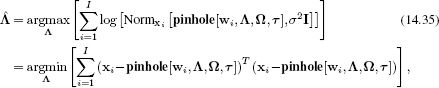
We now address the second problem. In camera calibration we attempt to learn the intrinsic parameters based on viewing a known object or calibration target. More precisely, we are given a known object, with I distinct 3D points {wi}Ii=1 and their corresponding 2D projections in the image {xi}Ii=1, and aim to form maximum likelihood estimates of the intrinsic parameters Λ,
![]()
A simple (but inefficient) approach to this problem is to use a coordinate ascent method in which we alternately
• Estimate the extrinsic parameters for fixed intrinsic parameters (problem 1),
![]()
using the procedure described in Section 14.4, and then
• Estimate the intrinsic parameters for fixed extrinsic parameters,
![]()
By iterating these two steps, we will get closer and closer to the correct solution. Since we already know how to solve the first of these two subproblems, we now concentrate on solving the second. Happily there is a closed form solution that does not even require homogeneous coordinates.
Given known world points {wi}iI=1, their projections {xi}iI=1, and known extrinsic parameters {Ω, τ}, our goal is now to compute the intrinsic matrix Λ, which contains the intrinsic parameters {![]() x,
x, ![]() y,γ, δx, δy}. We will apply the maximum likelihood method
y,γ, δx, δy}. We will apply the maximum likelihood method
which results in a least squares problem (see Section 4.4.1).
Now we note that the projection function pinhole[•, •, •, •] (Equation 14.8) is linear with respect to the intrinsic parameters, and can be written as Aih where
and h = [![]() x, γ, δx,
x, γ, δx, ![]() y, δy]T. Consequently, the problem has the form
y, δy]T. Consequently, the problem has the form
![]()
which we recognize as a least squares problem that can be solved in closed form (Appendix C.7.1).
We have described this alternating approach for pedagogical reasons; it is simple to understand and implement. However, we emphasize that this is not really a practical method as the convergence will be very slow. A better approach would be to perform a couple of iterations of this method and then optimize both the intrinsic and extrinsic parameters simultaneously using a nonlinear optimization technique such as the Gauss-Newton method (Appendix B.2.3) with the original criterion (Equation 14.32). This optimization must be done while ensuring that the extrinsic parameter Ω remains a valid rotation matrix (see Appendix B.4).
14.6 Inferring three-dimensional world points
Finally, we consider the multiview reconstruction problem. Given J calibrated cameras in known positions (i.e., cameras with known Λ, Ω, τ), viewing the same 3D point w and knowing the corresponding projections in the images {xj}Jj=1, establish the position of the point in the world.
![]()
This cannot be solved in closed form and so we move to homogeneous coordinates where we can solve for a good initial estimate in closed form. The relationship between the homogeneous world point ![]() and the jth corresponding homogeneous image point
and the jth corresponding homogeneous image point ![]() j is
j is
where we have appended the index j to the intrinsic and extrinsic parameters to denote the fact that they belong to the jth camera. Premultiplying both sides by the intrinsic matrix Λj-1 to convert to normalized image coordinates gives
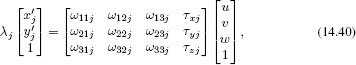
where x′j and y′j denote the normalized image coordinates in the jth camera.
We use the third equation to establish that ![]() . Substituting into the first two equations, we get
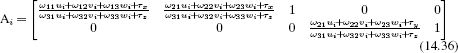
. Substituting into the first two equations, we get
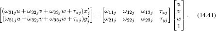
These equations can be rearranged to provide two linear constraints on the three unknown quantities in w =[u,v,w]T:
![]()
With multiple cameras, we can build a larger system of equations and solve for w in a least squares sense (Appendix C.7.1). This typically provides a good starting point for the subsequent nonlinear optimization of the criterion in Equation 14.38.
This calibrated reconstruction algorithm is the basis for methods that construct 3D models. However, there are several parts missing from the argument.
• The method requires us to have found the points {xj}Jj=1 that correspond to the same world point w in each of the J images. This process is called correspondence and is discussed in Chapters 15 and 16.
• The method requires the intrinsic and extrinsic parameters. Of course, these could be computed from a calibration target using the method of Section 14.5. However, it is still possible to perform reconstruction when the system is uncalibrated; this is known as projective reconstruction as the result is ambiguous up to a 3D projective transformation. Furthermore, if a single camera was used to take all of the images, it is possible to estimate the single intrinsic matrix and extrinsic parameters from a sequence, and reconstruct points in a scene up to a constant scaling factor. Chapter 16 presents an extended discussion of this method.
14.7 Applications
We discuss two applications for the techniques in this chapter. We consider a method to construct 3D models based on projecting structured light onto the object, and a method for generating novel views of an object based on an approximate model built from the silhouettes of the object.
14.7.1 Depth from structured light
In Section 14.6 we showed how to compute the depth of a point given its position in two or more calibrated cameras. However, we did not discuss how to find matching points in the two images. We defer a full answer to this question to Chapter 16, but here we will develop a method that circumvents this problem. This method will be based on a projector and a camera, rather than two cameras.
It is crucial to understand that the geometry of a projector is exactly the same as that of a camera: the projector has an optical center and has a regular pixel array that is analogous to the sensor in the camera. Each pixel in the projector corresponds to a direction in space (a ray) through the optical center, and this relationship can be captured by a set of intrinsic parameters. The major difference is that a projector sends outgoing light along these rays, whereas the camera captures incoming light along them.
Consider a system that comprises a single camera and a projector that are displaced relative to one another but that point at the same object (Figure 14.12). For simplicity, we will assume that the system is calibrated (i.e., the intrinsic matrices and the relative positions of the camera and projector are known). It is now easy to estimate the depth of the scene: we illuminate the scene using the projector one pixel at a time, and find the corresponding pixel in the camera by observing which part of the image gets brighter. We now have two corresponding points and can compute the depth using the method of Section 14.6. In practice, this technique is very time consuming as a separate image must be captured for each pixel in the projector. Scharstein and Szeliski(2003) used a more practical technique using structured light in which a series of horizontal and vertical stripe patterns is projected onto the scene that allow the mapping between pixels in the projector and those in the camera to be computed.
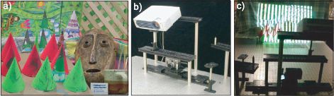
Figure 14.12 Depth maps from structured light. a) A three-dimensional scene that we wish to capture. b) The capture hardware consists of a projector and a camera, which both view the scene from different positions. c) The projector is used to illuminate the scene, and the camera records the pattern of illumination from its viewpoint. The resulting images contain information that can be used to compute a 3D reconstruction. Adapted from Scharstein and Szeliski(2003). ©2003 IEEE.
To understand how this works, consider a projector image in which the top half is light and the bottom half is dark. We capture two images I1 and I2 of the scene corresponding to when the projector shows this pattern and when it shows its inverse. We then take the difference I1 - I2 between the images. Pixels in the camera image where the difference is positive must now belong to the top half of the projector image, and pixels where the difference is negative must belong to the bottom half of the image. We now illuminate the image with a second pattern, which divides the images into four horizontally oriented black and white stripes. By capturing the image illuminated by this second pattern and its inverse, we can hence deduce whether each pixel is in the top or bottom half of the region determined by the first pattern. We continue in this way with successively finer patterns, refining the estimated position at each pixel until we know it accurately. The whole procedure is repeated with vertical striped patterns to estimate the horizontal position.
In practice, more sophisticated coding schemes are used as the sequence described in the preceding section; for example, this sequence means that there is always a boundary between black and white in the center of the projector image. It may be hard to establish the correspondence for a camera pixel, which always straddles this boundary. One solution is to base the sequences on Gray codes which have a more complex structure and avoid this problem (Figure 14.13). The estimated depth map of the scene in Figure 14.12 is shown in Figure 14.14.
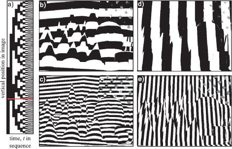
Figure 14.13 Projector to camera correspondence with structured light patterns. a) To establish the vertical position in the projector image, we present a sequence of horizontally striped patterns. Each height in the projected image receives a unique sequence of black and white values, so we can determine the height (e.g., red line) by measuring this sequence. b-c) Two examples of these horizontally striped patterns. d-e) Two examples of vertically striped patterns that are part of a sequence designed to estimate the horizontal position in the projector pattern. Adapted from Scharstein and Szeliski (2003). ©2003 IEEE.
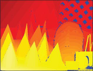
Figure 14.14 Recovered depth map for scene in Figure 14.12 using the structured light method. Pixels marked as blue are places where the depth is uncertain: these include positions in the image that were occluded with respect to the projector, so no light was cast onto them. Scharstein and Szeliski(2003) also captured the scene with two cameras under normal illumination; they subsequently used the depth map from the structured light as ground truth data for assessing stereo vision algorithms. Adapted from Scharstein and Szeliski(2003). ©2003 IEEE.
14.7.2 Shape from silhouette
The preceding system computed a 3D model of a scene based on explicit correspondences between a projector and a camera. We now consider an alternative method for computing 3D models that does not require explicit correspondence. As the name suggests, shape from silhouette estimates the shape of an object based on its silhouette in a number of images.
The principle is illustrated in Figure 14.15. Given a single camera, we know that an object must lie somewhere within the bundle of rays that fall within its silhouette. Now consider adding a second camera. We also know that the object must lie somewhere within the bundle of rays corresponding to the silhouette in this image. Hence, we can refine our estimate of the shape to the 3D intersection of these two ray bundles. As we add more cameras, the possible region of space that the object can lie in is reduced.
This procedure is attractive because the silhouettes can be computed robustly and quickly using a background subtraction approach. However, there is also a downside; even if we have an infinite number of cameras viewing the object, some aspects of the shape will not be present in the resulting 3D region. For example, the concave region at the back of the seat of the chair in Figure 14.15a cannot be recovered as it is not represented in the silhouettes. In general, the “best possible” shape estimate is known as the visual hull.
We will now develop an algorithm based on shape from silhouette that can be used to generate images of an object from novel poses. One application of this is for augmented reality systems in which we wish to superimpose an object over a real image in such a way that it looks like it is a stable part of the scene. This can be accomplished by establishing the position and pose of the camera relative to the scene (Section 14.4) and then generating a novel image of the object from the same viewpoint. Figure 14.17 depicts an example application of this kind, in which the performance of an actor is captured and rebroadcast as if he is standing on the desk.
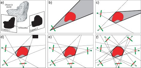
Figure 14.15 Shape from silhouette. a) The goal is to recover information about the shape of the object based on the silhouettes in a number of cameras. b) Consider a single camera viewing an object (2D slice shown). We know that the object must lie somewhere within the shaded region defined by the silhouette. c) When we add a second camera, we know that the object must lie within the intersection of the regions determined by the silhouettes (gray region). d-f) As we add more cameras, the approximation to the true shape becomes closer and closer. Unfortunately, we can never capture the concave region, no matter how many cameras we add.
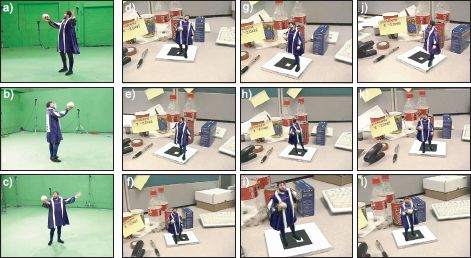
Figure 14.16 Generating novel views. a-c) An actor is captured from 15 cameras in a green screen studio. d-l) Novel views of the actor are now generated and superimposed on the scene. The novel view is carefully chosen so that it matches the direction that the camera views the desktop giving the impression that the actor is a stable part of the scene. Adapted from Prince et al. (2002). ©2002 IEEE.
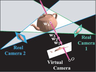
Figure 14.17 Novel view generation. A new image is generated one pixel at a time by testing a sequence of points w1,w2,… along the ray through the pixel. Each point is tested to see if it is within the visual hull by projecting it into the real images. If it lies within the silhouette in every real image, then it is within the visual hull and the search stops. In this case, point wk is the first point on the surface. To establish the color for the pixel, this point is projected into a nearby real image, and the color is copied. Adapted from Prince et al. (2002). ©2002 IEEE.
Prince et al. (2002) described a method to generate a novel image from a virtual camera with intrinsic matrix Λ and extrinsic parameters Λ {Ω, τ}. They considered each pixel in the virtual camera in turn, and computed the direction of the ray r passing through this point. With respect to the virtual camera itself, this ray has a direction
![]()
where ![]() is the position of the point in the image expressed in homogeneous coordinates. With respect to the global coordinate system, a point w that is k units along the ray can be expressed as
is the position of the point in the image expressed in homogeneous coordinates. With respect to the global coordinate system, a point w that is k units along the ray can be expressed as
![]()
The depth of the object at this pixel is then computed by exploring along this direction; it is determined by an explicit search starting at the virtual camera projection center and proceeding outward along the ray corresponding to the pixel center (Figure 14.17). Each candidate 3D point along this ray is evaluated for potential occupancy. A candidate point is unoccupied if its projection into any of the real images is marked as background. When the first point is found for which all of the projected positions are marked as foreground, this is considered the depth with respect to the virtual object and the search stops.
The 3D point where the ray through the current virtual pixel meets the visual hull is now known. To establish the color of this pixel in the virtual image, the point is projected into the closest real image, and the color is copied. In general, the projection will not be exactly centered on a pixel, and to remedy this, the color value is estimated using bilinear or bicubic interpolation.
This procedure can be accomplished very quickly; the system of Prince et al. (2002) depicted in Figure 14.16 ran at interactive speeds, but the quality is limited to the extent that the visual hull is a reasonable approximation of the true shape. If this approximation is bad, the wrong depth will be estimated, the projections into the real images will be inaccurate, and the wrong color will be sampled.
Discussion
In this chapter, we have introduced a model for a pinhole camera and discussed learning and inference algorithms for this model. In the next chapter, we consider what happens when this camera views a planar scene; here there is a one-to-one mapping between points in the scene and points in the image. In Chapter 16, we return to the pinhole camera model and consider reconstruction of a scene from multiple cameras in unknown positions.
Notes
Camera geometry: There are detailed treatments of camera geometry in Hartley and Zisserman (2004), Ma et al. (2004), and Faugeras et al. (2001). Aloimonos (1990) and Mundy and Zisserman (1992) developed a hierarchy of camera models (see Problem 14.3). Tsai (1987) and Faugeras (1993) both present algorithms for camera calibration from a 3D object. However, it is now more usual to calibrate cameras from multiple images of a planar object (see Section 15.4) due to the difficulties associated with accurately machining a 3D object. For a recent summary of camera models and geometric computer vision, consult Sturm et al. (2011).
The projective pinhole camera discussed in this chapter is by no means the only camera model used in computer vision; there are specialized models for the pushbroom camera (Hartley and Gupta 1994), fish-eye lenses (Devernay and Faugeras 2001; Claus and Fitzgibbon 2005), catadioptric sensors (Geyer and Daniilidis 2001; M![]() cušík and Pajdla 2003; Claus and Fitzgibbon 2005), and perspective cameras imaging through an interface into a medium (Treibitz et al. 2008).
cušík and Pajdla 2003; Claus and Fitzgibbon 2005), and perspective cameras imaging through an interface into a medium (Treibitz et al. 2008).
Estimating extrinsic parameters: A large body of work addresses the PnP problem of estimating the geometric relation between the camera and a rigid object. Lepetit et al. (2009) present a recent approach that has low complexity with respect to the number of points used and provides a quantitative comparison with other approaches. Quan and Lan (1999) and Gao et al. (2003) present minimal solutions based on three points.
Structured light: The structured light method discussed in this chapter is due to Scharstein and Szeliski (2003), although the main goal of their paper was to generate ground truth for stereo vision applications. The use of structured light has a long history in computer vision (e.g., Vuylsteke and Oosterlinck 1990), with the main research issue being the choice of pattern to project (Salvi et al. 2004; Batlle et al. 1998; Horn and Kiryati 1999).
Shape from silhouette: The recovery of shape from multiple silhouettes of an object dates back to at least Baumgart (1974). Laurentini (1994) introduced the concept of the visual hull and described its properties. The shape from silhouette algorithm discussed in this chapter was by Prince et al. (2002) and is closely related to earlier work by Matusik et al. (2000) but rather simpler to explain. Recent work in this area has considered a probabilistic approach to pixel occupancy (Franco and Boyer 2005), the application of human silhouette priors (Grauman et al. 2003), the use of temporal sequences of silhouettes (Cheung et al. 2004), and approaches that characterize the intrinsic projective features of the visual hull.
Human performance capture: Modern interest in human performance capture was stimulated by Kanade et al. (1997). More recent work in this area includes that of Starck et al. (2009), Theobalt et al. (2007), Vlasic et al. (2008), de Aguiar et al. (2008), and Ballan and Cortelazzo (2008).
Problems
14.1 A pinhole camera has a sensor that is 1 cm × 1 cm and a horizontal field of view of 60°. What is the distance between the optical center and the sensor? The same camera has a resolution of 100 pixels in the horizontal direction and 200 pixels in the vertical direction (i.e., the pixels are not square). What are the focal length parameters fx and fy from the intrinsic matrix?
14.2 We can use the pinhole camera model to understand a famous movie effect. Dolly zoom was first used in Alfred Hitchcock’s Vertigo. As the protagonist looks down a stairwell, it appears to deform (Figure 14.18) in a strange way. The background seems to move away from the camera, while the foreground remains at a constant position.
In terms of the camera model, two things occur simultaneously during the dolly zoom sequence: the camera moves along the w-axis, and the focal distance of the camera changes. The distance moved and the change of focal length are carefully chosen so that objects in a predefined plane remain at the same position. However, objects out of this plane move relative to one another (Figures 14.18d-e).
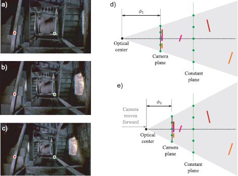
Figure 14.18 Dolly zoom. a-c) Three frames from Vertigo in which the stairwell appears to distort. Nearby objects remain in roughly the same place whereas object further away systematically move through the sequence. To see this, consider the red and green circles which are at the same (x,y) position in each frame. The red circle remains on the near bannister, but the green circle is on the floor of the stairwell in the first image but halfway up the stairs in the last image. d) To understand this effect consider a camera viewing a scene that consists of several green points at the same depth and some other surfaces (colored lines). e) We move the camera along the w-axis but simultaneously change the focal length so that the green points are imaged at the same position. Under these changes, objects in the plane of the green points are static, but other parts of the scene move and may even occlude one another.
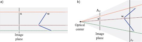
Figure 14.19 Alternative camera models. a) Orthographic camera. Rays are parallel and orthogonal to image plane. b) Weak perspective model. Points are projected orthogonally onto a reference plane at distance zr from the camera and then pass to the image plane by perspective projection.
I want to capture two pictures of a scene at either end of a dolly zoom. Before the zoom, the camera is at w = 0, the distance between the optical center and the image plane is 1 cm, and the image plane is 1 cm × 1cm. After the zoom, the camera is at w = 100 cm. I want the plane at w = 500 cm to be stable after the camera movement. What should the new distance between the optical center and the image plane be?
14.3 Figure 14.19 shows two different camera models: the orthographic and weak perspective cameras. For each camera, devise the relationship between the homogeneous world points and homogeneous image points. You may assume that the world coordinate system and the camera coordinate system coincide, so there is no need to introduce the extrinsic matrix.
14.4 A 2D line can be as expressed as ax+by+c = 0 or in homogeneous terms
![]()
where l = [a,b,c]. Find the point where the homogeneous lines l1 and l2 join where:
1. l1 = [3, 1, 1], and l2 = [-1, 0, 1]
2. l1 = [1, 0, 1], and l2 = [3, 0, 1]
Hint: the 3×1 homogeneous point vector ![]() must satisfy both l1
must satisfy both l1![]() =0 and l2
=0 and l2![]() =0. In other words it should be orthogonal to both l1 and l2.
=0. In other words it should be orthogonal to both l1 and l2.
14.5 Find the line joining the homogeneous points ![]() and
and ![]() where
where
![]()
14.6 A conic C is a geometric structure that can represent ellipses and circles in the 2D image. The condition for a point to lie on a conic is given by
![]()
or
![]()
Describe an algorithm to estimate the parameters a,b,c,d,e,f given several points x1,x2,…,xn that are known to lie on the conic. What is the minimum number of points that your algorithm requires to be successful?
14.7 Devise a method to find the intrinsic matrix of a projector using a camera and known calibration object.
14.8 What is the minimum number of binary striped light patterns of the type illustrated in Figure 14.13 required to estimate the camera-projector correspondences for a projector image of size H × W?
14.9 There is a potential problem with the shape from silhouette algorithm as described; the point that we have found on the surface of the object may be occluded by another part of the object with respect to the nearest camera. Consequently, when we copy the color, we will get the wrong value. Propose a method to circumvent this problem.
14.10 In the augmented reality application (Figure 14.16), the realism might be enhanced if the object had a shadow. Propose an algorithm that could establish whether a point on the desktop (assumed planar) is shadowed by the object with respect to a point light source at a known position.
___________________________________
1 This is not an accidental choice of word. The term camera is derived from the Latin word for ‘chamber.’
2 It should be noted that in practice calibration is more usually based on a number of views of a known 2D planar object (see Section 15.4.2).
All materials on the site are licensed Creative Commons Attribution-Sharealike 3.0 Unported CC BY-SA 3.0 & GNU Free Documentation License (GFDL)
If you are the copyright holder of any material contained on our site and intend to remove it, please contact our site administrator for approval.
© 2016-2026 All site design rights belong to S.Y.A.