Computer Vision: Models, Learning, and Inference (2012)

In most of the models in this book, the observed data are treated as continuous. Hence, for generative models the data likelihood is usually based on the normal distribution. In this chapter, we explore generative models that treat the observed data as discrete. The data likelihoods are now based on the categorical distribution; they describe the probability of observing the different possible values of the discrete variable.

As a motivating example for the models in this chapter, consider the problem of scene classification (Figure 20.1). We are given example training images of different scene categories (e.g., office, coastline, forest, mountain) and we are asked to learn a model that can classify new examples. Studying the scenes in Figure 20.1 demonstrates how challenging a problem this is. Different images of the same scene may have very little in common with one another, yet we must somehow learn to identify them as the same. In this chapter, we will also discuss object recognition, which has many of the same characteristics; the appearance of an object such as a tree, bicycle, or chair can vary dramatically from one image to another, and we must somehow capture this variation.

The key to modeling these complex scenes is to encode the image as a collection of visual words, and use the frequencies with which these words occur as the substrate for further calculations. We start this chapter by describing this transformation.

20.1 Images as collections of visual words

To encode an image in terms of visual words, we need first to establish a dictionary. This is computed from a large set of training images that are unlabeled, but known to contain examples of all of the scenes or objects that will ultimately be classified. To compute the dictionary, we take the following steps:

1. For every one of the I training images, select a set of J_i spatial locations. One possibility is to identify interest points (Section 13.2) in the image. Alternately, the image can be sampled in a regular grid.

2. Compute a descriptor at each spatial location in each image that characterizes the surrounding region with a low dimensional vector. For example, we might compute the SIFT descriptor (Section 13.3.2).

3. Cluster all of these descriptor vectors into K groups using a method such as the K-means algorithm (Section 13.4.4).

4. The means of the K clusters are used as the K prototype vectors in the dictionary.

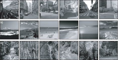
Figure 20.1 Scene recognition. The goal of scene recognition is to assign a discrete category to an image according to the type or content. In this case, the data includes images of a) street scenes, b) the sea, and c) forests. Scene recognition is a useful precursor to object recognition; if we know that the scene is a street, then the probability of a car being present is high, but the probability of a boat being present is small. Unfortunately, scene recognition is quite a challenging task in itself. Different examples from the same scene class may have very little in common visually.

Typically, several hundred thousand descriptors would be used to compute the dictionary, which might consist of several hundred prototype words.

Having computed the dictionary, we are now in a position to take a new image and convert it into a set of visual words. To compute the visual words, we take the following steps:

1. Select a set of J spatial locations in the image using the same method as for the dictionary.

2. Compute the descriptor at each of the J spatial locations.

3. Compare each descriptor to the set of K prototype descriptors in the dictionary and find the closest prototype (visual word).

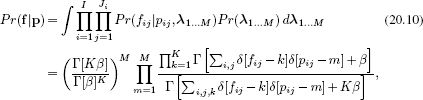
4. Assign to this location a discrete index that corresponds to the index of the closest word in the dictionary.

After computing the visual words, the data x from a single image consist of a set x = {f_j, x_j, y_j}^J_j=1 of J word indices f_j∈{1…K} and their 2D image positions (x_j,y_j). This is a highly compressed representation that nonetheless contains the critical information about the image appearance and layout. In the remaining part of the chapter, we will develop a series of generative models that attempt to explain the pattern of this data when different objects or scenes are present.

20.2 Bag of words

One of the simplest possible representations for an image in terms of visual words is the bag of words. Here we entirely discard the spatial information held in the word positions (x_j, y_j) and just retain the word indices f_j, so that the observed data are x = {f_j}^J_j=1. The image is simply represented by the frequency with which each word appears. It is assumed that different types of object or scene will tend to contain different words and that this can be exploited to perform scene or object recognition (Figure 20.2).

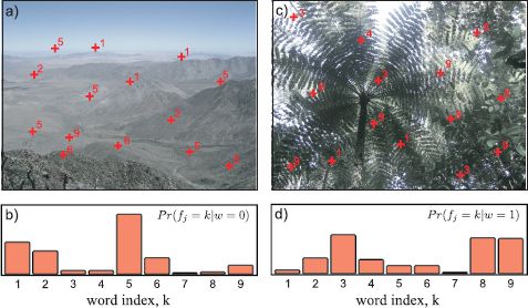
Figure 20.2 Scene recognition using bags of words. a) A set of interest points is found in this desert scene and a descriptor is calculated at each. These descriptors are compared to a dictionary containing K prototypes and the index of the nearest prototype is chosen (red numbers). Here K=9, but in real applications it might be several hundred. b) The scene-type “desert” implies a certain distribution over the observed visual words. c) A second image containing a jungle scene, and the associated visual words. d) The scene type “jungle” implies a different distribution over the visual words. A new image can be classified as belonging to one scene type or another by assessing the likelihood that the observed visual words were drawn from the “desert” or “jungle” distribution.

More formally, the goal is to infer a discrete variable w ∈{1,2,…,N} indicating which of N classes is present in this image. We take a generative approach and model each of the N classes separately. Since the data {f_j}^J_j=1 are discrete, we describe its probability with a categorical distribution and make the parameters λ of this distribution a function of the discrete world state:

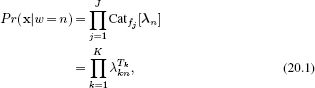
where T_k is the total number of times that the k^th word was observed, so that

We will now consider the learning and inference algorithms for this model.

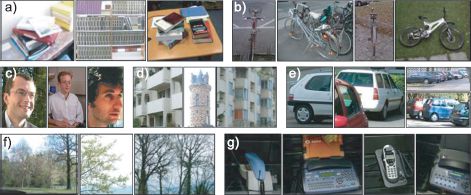
Figure 20.3 Object recognition using bags of words. Csurka et al. (2004) built a generative bag of visual words model to distinguish between examples of a) books, b) bicycles, c) people, d) buildings, e) cars, f) trees, and g) phones. Despite the wide variety of visual appearance within each class, they achieved 72 percent correct classification. By applying a discriminative approach to the same problem, they managed to improve performance further.

20.2.1 Learning

In learning, our goal is to estimate the parameters {λ_n}^N_n=1 based on labeled pairs {x_i,w_i} of the observed data x_i={f_ij}^J_ij=1 and the world state w_i. We note that the n^th parameter vector λ_n is used only when the world state w_i = n. Hence, we can learn each parameter vector separately; we learn the parameter λ_n from the subset _n of training images where w_i = n.

Making use of the results in Section 4.5, we see that if we apply a Dirichlet prior with uniform parameter α = [α,α,…,α], then the MAP estimate of the categorical parameters is given by

where λ_nk is the k^th entry in the categorical distribution for the n^th class and T_ik is the total number of times that word k was observed in the i^th training image.

20.2.2 Inference

To infer the world state, we apply Bayes’ rule:

where we allocate suitable prior probabilities Pr(w = n) according to the relative frequencies with which each world type is present.

Discussion

Despite discarding all spatial information, the bag of words model works remarkably well for object recognition. From example, Csurka et al. (2004) achieved 72 percent correct performance at classifying images of the seven classes found in Figure 20.3. It should be noted that it is possible to improve performance further by treating the vector z =[T₁,T₂,…,T_K]/∑_kT_k of normalized word frequencies as continuous and subjecting it to a kernelized discriminative classifier (see Chapter 9). Regardless, we will continue to investigate the (more theoretically interesting) generative approach.

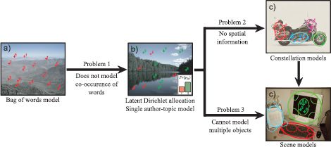
Figure 20.4 Problems with bag of words model. a) The bag of words model is quite effective for object and scene recognition, but it can be improved upon by b) modeling the cooccurence of visual words (creating the latent Dirichlet allocation model). c) This model can be extended to describe the relative positions of different parts of the object (creating a constellation model) and d) extended again to describe the relative position of objects in the scene (creating a scene model).

20.2.3 Problems with the bag of words model

There are a number of drawbacks to the generative bag of words model:

• It assumes that the words are generated independently, within a given object class although this is not necessarily true. The presence of a particular visual word tells us about the likelihood of observing other words.

• It ignores spatial information; consequently, when applied to object recognition, it cannot tell us where the object is in the image.

• It is unsuited to describing multiple objects in a single image.

We devote the remaining part of this chapter to building a series of generative models that improve on these weaknesses (Figure 20.4).

20.3 Latent Dirichlet allocation

We will now develop an intermediate model known as latent Dirichlet allocation. This model has limited utility for visual applications in its most basic form, but it underpins more interesting models that are discussed subsequently.

There are two important differences between the bag of words and latent Dirichlet allocation models. First, the bag of words model describes the relative frequency of visual words in a single image, whereas latent Dirichlet allocation describes the occurrence of visual words across a number of images. Second, the bag of words model assumes that each word in the image is generated completely independently; having observed word f_i1, we are none the wiser about word f_i2. However, in the latent Dirichlet allocation model, a hidden variable associated with each image induces a more complex distribution over the word frequencies.

Latent Dirichlet allocation can be best understood by analogy to text documents. Each document is considered as a certain mixture of topics. For example, this book might contain the topics “machine learning”, “vision,” and “computer science” in proportions of 0.3, 0.5, and 0.2, respectively. Each topic defines a probability distribution over words; the words “image” and “pixel” might be more probable under the topic of vision, and the words “algorithm” and “complexity” might be more probable under the topic of computer science.

To generate a word, we first choose a topic according to the topic probabilities for the current document. Then we choose a word according to a distribution that depends on the chosen topic. Notice how this model induces correlations between the probability of observing different words. For example, if we see the word “image”, then this implies that the topic “vision” has a significant probability and hence observing the word “pixel” becomes more likely.

Now let us convert these ideas back to the vision domain. The document becomes an image, and the words become visual words. The topic does not have an absolutely clear interpretation, but we will refer to it as a part. It is a cluster of visual words that tend to co-occur in images. They may or may not be spatially close to one another in the image, and they may or may not correspond to an actual “part” of an object (Figure 20.5).

Formally, the model represents the words in an image as a mixture of categorical distributions. The mixing weights depend on the image, but the parameters of the categorical distributions are shared across all of the images:

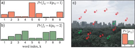
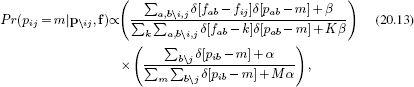
Figure 20.5 Latent Dirichlet allocation. This model treats each word as belonging to one of M different parts (here M = 2). a) The distribution over the words given that the part is 1 is described by a categorical distribution. b) The distribution over the words given that the part is 2 is described by a different categorical distribution. c) In each image, the tendency for the observed words to belong to each part is different. In this case, part 1 is more likely than part 2 and so most of the words belong to part 1 (are red as opposed to green).

where i indexes the image and j indexes the word. The first equation says that the part label p_ij ∈ {1,2,…, M} associated with the j^th word in the i^th image is drawn from a categorical distribution with parameters π_i that are unique to this image. The second equation says that the actual choice of visual word f_ij is a categorical distribution where the parameters λ_pij depend on the part. For short, we will refer to {π_i}^I_i=1 and {λ_m}^M_m=1 as the part probabilities and the word probabilities, respectively.

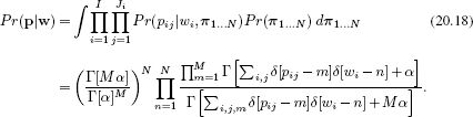
The final density over the words comes from marginalizing over the part labels, which are hidden variables, so that

To complete the model, we define priors on the parameters {π_i}^I_i=1, {λ_m}^M_m=1, where I is the number of images and M is the total number of parts. In each case, we choose the conjugate Dirichlet prior with a uniform parameter vector so that

where α = [α,α,…,α] and β = [β, β, …, β]. The associated graphical model is shown in Figure 20.6.

Notice that latent Dirichlet allocation is a density model for the data in a set of images. It does not involve a “world” term that we wish to infer. In the subsequent models, we will reintroduce the world term and use the model for inference in visual problems. However, for now we will concentrate on how to learn the relatively simple latent Dirichlet allocation model.

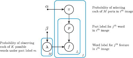
Figure 20.6 Graphical model for latent Dirichlet allocation. The likelihood of the j^th word f_ij in the i^th image taking each of the K different values depends on which of M parts it belongs to, and this is determined by the associated part label p_ij. The tendency of the part label to take different values is different for each image and is determined by the parameters π_i. The hyperparameters α and β determine the Dirichlet priors over the part probabilities and word probabilities, respectively.

20.3.1 Learning

In learning, the goal is to estimate the part probabilities {π_i}^I_i=1 for each of the I training images and the word probabilities for each of the M parts {λ_m}^M_m=1 based on a set of training data {f_ij}^I,J_ii=1,j=1, where J_i denotes the number of words found in the i^th image.

If we knew the values of the hidden part labels {p_ij}_i=1,j=1^I,J_i, then it would be easy to learn the unknown parameters. Adopting the approach of Section 4.4, the exact expressions would be

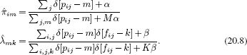
Unfortunately, we do not know these part labels and so we cannot use this direct technique. One possible approach would be to adopt the EM algorithm in which we alternately compute the posterior distribution over the part labels and update the parameters. Unfortunately, this is also problematic; all of the part labels {p_ij}^J_ij=1 in the i^th image share a parent π_i in the graphical model. This means we cannot treat them as independent. In theory, we could compute their joint posterior distribution, but there may be several hundred words per image, each of which takes several hundred values and so this is not practical.

Hence, our strategy will be to:

• Write an expression for the posterior distribution over the part labels,

• Develop an MCMC method to draw samples from this distribution, and then

• use the samples to estimate the parameters.

These three steps are expanded upon in the next three sections.

Posterior distribution over part labels

The posterior distribution over the part labels p = {p_ij}^I,J_ii=1,j=1 results from applying Bayes’ rule:

where f = {f_ij}^I,J_ii=1,j=1 denotes the observed words.

The two terms in the numerator depend on the word probabilities {λ_m}^M_m=1 and the part probabilities {π_i}^I_i=1, respectively. However, since each of these quantities has a conjugate prior, we can marginalize over them and remove them from the computation entirely. Hence, the likelihood Pr(f|p) can be written as

and the prior can be written as

where we exploited conjugate relations to help solve the integral (see Problem 3.10).

Unfortunately, we cannot compute the denominator of Equation 20.9 as this involves summing over every possible assignment of the word labels f. Consequently, we can only compute the posterior probability for part labels p up to an unknown scaling factor. We encountered a similar situation before in the MRF labeling problem (Chapter 12). In that case there was a polynomial time algorithm to find the MAP estimate, but here that is not possible; the cost function for this problem cannot be expressed as a sum of unary and pairwise terms.

Drawing samples from posterior distribution

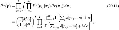
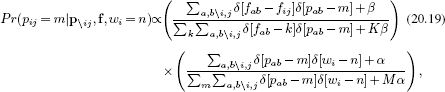
To make progress, we will use a Monte Carlo Markov chain method to generate a set of samples {p^[1]p^[2],…, p^[T]} from the posterior distribution. More specifically, we will use a Gibbs sampling approach (see Section 10.7.2) in which we update each part label p_ij in turn. To do this, we compute the posterior probability of the current part label assuming that all of the others are fixed and then draw a sample from this distribution. We repeat this for every part label to generate a new sample of p. This posterior probability of a single part label assuming that the others are fixed has M elements that are computed as

where the notation p_\ij denotes all of the elements of p except p_ij. To estimate this, we must compute joint probabilities Pr(f,p) = Pr(f|p)Pr(p) using Equations 20.10 and 20.11. In practice, the resulting expression simplifies considerably to

where the notation ∑_a,b\i,j means sum over all values of {a,b} except i,j. Although it looks rather complex, this expression has a simple interpretation. The first term is the probability of observing the word f_ij given that part p_ij = m. The second term is the proportion of the time that part m is present in the current document.

To sample from the posterior distribution, we initialize the part labels {p_ij}^I,J_ii=1,j=1 and alternately update each part label in turn. After a reasonable burn in period (several thousand iterations over all of the variables), the resulting samples can be assumed to be drawn from the posterior. We then take a subset of samples from this chain, where each is separated by a reasonable distance to ensure that their correlation is low.

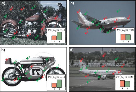
Figure 20.7 Single author-topic model. The single author-topic model is a variant of latent Dirichlet allocation that includes a variable w_i ∈ {1…N} that represents which of N possible objects is in the image. It is assumed that the part probabilities {π_n}^N_n=1 are contingent on the particular choice of object. a) Image 1 contains a motorbike and this induces the part probabilities shown in the bottom right hand corner. The parts are drawn from this probability distribution (color of crosses) and the words (numbers) are drawn based on the parts chosen. b) A second image of a motorbike induces the same part probabilities. c-d) These two images contain a different object and hence have different part probabilities (bottom right).

Using samples to estimate parameters

Finally, we estimate the unknown parameters using the expressions

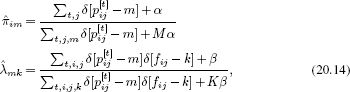
which are very similar to the original expressions (Equation 20.8) for estimating the parameters given known part labels.

20.3.2 Unsupervised object discovery

The preceding model can been used to help analyze the structure of a set of images. Consider fitting this model to an unlabeled data set containing several images each of a number of different object categories. After fitting, each of the I images is modeled as a mixture of parts, and we have an estimate of the mixture weights λ_i for each. We now cluster the images according to the dominant part in this mixtures. For small data sets, it has been shown that this method can separate out different object classes with a high degree of accuracy; this model allows the discovery of object classes in unlabeled data sets.

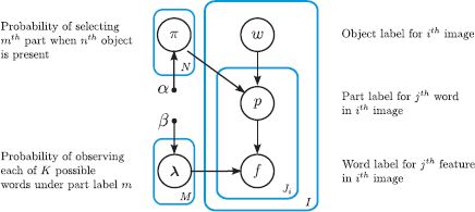
Figure 20.8 Graphical model for the single author-topic model. The likelihood of the j^th word in the i^th image f_ij being categorized as one word or another depends on which of M parts it belongs to, and this is determined by the associated part label p_ij. The tendency of the part label to take different values is different for each object w_i ∈ {1…N} is determined by the parameters π_n, where it is assumed there is a single object in each image.

20.4 Single author-topic model

Latent Dirichlet allocation is simply a density model for images containing sets of discrete words. We will now describe an extension to this model that assumes there is a single object in each image, and the identity of this object is characterized by a label w_i ∈ {1…N}. In the single author-topic model (Figure 20.7), we make the assumption that each image of the same object contains the same part probabilities:

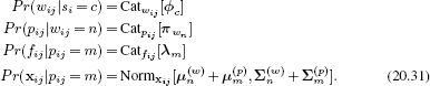
To complete the model, we add Dirichlet priors to the unknown parameters {π_n}^N_n=1 and {λ_m}^M_m=1:

where α = [α,α,…, α] and β = [β,β,…,β]. For simplicity we will assume that the prior over the object label w is uniform and not discuss this further. The associated graphical model is illustrated in Figure 20.8.

Like the bag of words and latent Dirichlet allocation models, this model was originally used for describing text documents; it assumes that each document was written by one author (each image contains one object), and this determines the relative frequency of topics (of parts). It is a special case of the more general author-topic model, which allows multiple authors for each document.

20.4.1 Learning

Learning proceeds in much the same way as in latent Dirichlet allocation. We are given a set of I images, each of which has a known object label w_i ∈ {1…N} and a set of visual words {f_ij}^J_ij=1, where f_ij ∈{1…M}. It would be easy to estimate the part probabilities for each object {π_n}^N_n=1 and the word probabilities for each part {λ_m}^M_m=1 if we knew the hidden part labels p_ij associated with each word. As before we take the approach of drawing samples from the posterior distribution over the part labels and using these to estimate the unknown parameters. This posterior is computed via Bayes’ rule:

where w = {w_i}^I_i=1 contains all of the object labels.

The likelihood term Pr(f|p) is the same as for latent Dirichlet allocation and is given by Equation 20.10. The prior term becomes

As before, we cannot compute the denominator of Bayes’ rule as it involves an intractable summation over all possible words. Hence, we use a Gibbs sampling method in which we repeatedly draw samples p^[1]… p^[T] from each marginal posterior in turn using the relation:

where the notation ∑_a,b\i,j denotes a sum over all valid values of a,b except for the combination i,j. This expression has a simple interpretation. The first term is the probability of observing the word f_ij given that part p_ij = m. The second term is the proportion of the time that part m is present for the n^th object.

Finally, we estimate the unknown parameters using the relations:

20.4.2 Inference

In inference, we compute the likelihood of new image data f = {f_j}^J_j=1 under each possible object w ∈ {1…N} using

We now define suitable priors Pr(w) over the possible objects and use Bayes’ rule to compute the posterior distribution,

20.5 Constellation models

The single author-topic model described in Section 20.4 is still a very weak description of an object as it contains no spatial information. Constellation models are a general class of model that describe objects in terms of a set of parts and their spatial relations. For example, the pictorial structures model described in Section 11.8.3 can be considered a constellation model. Here, we will develop a different type of constellation model that extends the latent Dirichlet allocation model (Figure 20.9).

We assume that a part retains the same meaning as before; it is a cluster of co-occurring words. However, each part now induces a spatial distribution over its associated words, which we will model with a 2D normal distribution so that

where x_ij = [x_ij,y_ij]^T is the two-dimensional position of the j^th word in the i^th image. As before, we also define Dirichlet priors over the unknown categorical parameters so that

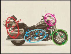
Figure 20.9 Constellation model. In the constellation model the object or scene is again described as consisting of set of different parts (colors). A number of words are associated with each part, and the word probabilities depend on the part label. However, unlike in the previous models, each part now has a particular range of locations associated with it, which are described as a normal distribution. In this sense it conforms more closely to the normal use of the English word “part.”

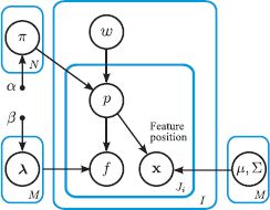
Figure 20.10 Constellation model. In addition to all of the other variables in the single author-topic model (compare to Figure 20.8), the position x_ij of the j^th word in the i^th image is also modeled. This position is contingent on which of the M parts that the current word is assigned to (determined by the variable p_ij). When the word is assigned to the m^th part, the position x_ij is modeled as being drawn from a normal distribution with mean and variance μ_m, ∑_m.

where α = [α,α,…,α] and β = [β,β,…,β]. The associated graphical model is shown in Figure 20.10.

This model extends latent Dirichlet allocation to allow it to represent the relative positions of parts of an object or scene. For example, it might learn that words associated with trees usually occur in the center of the image and that those associated with the sky usually occur near the top of the image.

20.5.1 Learning

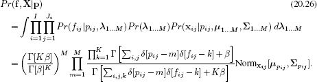
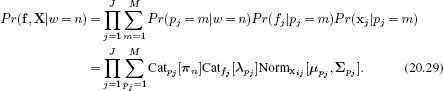
As for latent Dirichlet allocation, the model would be easy to learn if we knew the part assignments p = {p_ij}^I,J_ii=1,j=1. By the same logic as before, we hence draw samples from posterior distribution Pr(p|f,X,w) over the part assignments given the observed word labels f = {f_ij},_j=1^I,J_i, their associated positions X = {x_ij}^I,J_ii=1,j=1, and the known object labels w = {w_i}^I_i=1. The expression for the posterior is computed via Bayes’ rule

and once again, the terms in the numerator can be computed, but the denominator contains an intractable sum of exponentially many terms. This means that the posterior cannot be computed in closed form, but we can still evaluate the posterior probability for any particular assignment p up to an unknown scale factor. This is sufficient to draw samples from the distribution using Gibbs sampling.

The prior probability Pr(p|w) of the part assignments is the same as before and is given in Equation 20.18. However, the likelihood term Pr(f,X|p) now has an additional component due to the requirement for the word position x_ijto agree with the normal distribution induced by the part:

In Gibbs sampling, we choose one data example {f_ij,x_ij} and draw from the posterior distribution assuming that all of the other parts are fixed. An approximate¹ expression to compute this posterior is given by

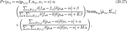
where the notation ∑_a,b\i,j denotes summation over all values of {a,b} except i,j. The terms _m and _m are the mean and covariance of all of the word positions associated with the m^th part ignoring the contribution of the current position x_ij.

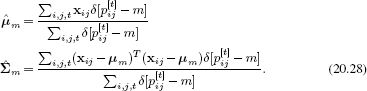
At the end of the procedure, the probabilities are computed using the relations in Equation 20.20 and the part locations as

Example learning results can be seen in Figure 20.11. Each part is a spatially localized cluster of words, and these often correspond to real-world objects such as “legs” or “wheels.” The parts are shared between the objects and so there is no need for a different set of parameters to learn the appearance of wheels for bicycles and wheels for motorbikes.

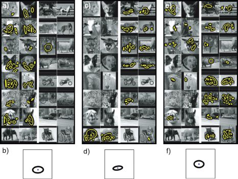
Figure 20.11 Sharing words in the constellation model. a) Sixteen images from training set (two from each class). Yellow ellipses depict words identified in the image associated with one part of the image (i.e., they are equivalent of the crosses in Figure 20.9). It is notable that the words associated with this part mainly belong to the lower part of the faces of the animal images. b) The mean μ and variance ∑ of this object part. c,d) A second part seems to correspond to the legs of animals in profile. e,f) A third part contains many words associated with the wheels of objects. Adapted from Sudderth et al. (2008). ©2008 IEEE.

20.5.2 Inference

In inference, we compute the likelihood of new image data {f_j, x_j}^J_j=1 under each possible object w ∈ {1…N} using

We now define suitable priors Pr(w) over the possible objects and use Bayes’ rule to compute the posterior distribution

20.6 Scene models

One limitation of the constellation model is that it assumes that the image contains a single object. However, real images generally contain a number of spatially offset objects. Just as the object determined the probability of the different parts, so the scene determines the relative likelihood of observing different objects (Figure 20.12). For example, an office scene might include desks, computers, and chairs, but it is very unlikely to include tigers or icebergs.

To this end we introduce a new set of variables that represent the choice of scene {_i}^I_i=1 ∈ {1…C}

Each word has an object label {w_ij}^I,J_Ii=1,j=1, which denotes which of the L objects it corresponds to. The scene label {_i} determines the relative propensity for each object to be present, and these probabilities are held in the categorical parameters {_c}^C_c=1. Each object type also has a position that is normally distributed with mean and covariance μ_m^(w) and ∑_m^(w). As before, each object defines a probability distribution over the M shared parts where the part assignment is held in the label p_ij. Each part has a position that is measured relative to the object position and has mean and covariance μ^(p)_m, and ∑^(p)_m, respectively.

We leave the details of the learning and inference algorithms as an exercise for the reader; the principles are the same as for the constellation model; we generate a series of samples from the posterior over the hidden variables w_ijand p_ij using Gibbs sampling and update the mean and covariances based on the samples.

Figure 20.13 shows several examples of scenes that have been interpreted using a scene model very similar to that described. In each case, the scene is parsed into a number of objects that are likely to co-occur and are in a sensible relative spatial configuration.

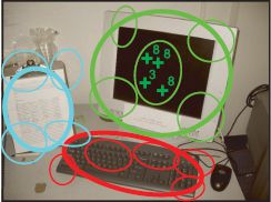
Figure 20.12 Scene model. Each image consists of a single scene. A scene induces a probability distribution over the presence of different objects (different colors) such as the monitor, piece of paper, and keyboard in this scene and their relative positions (thick ellipses). Each object is itself composed of spatially separate parts (thin ellipses). Each part has a number of words associated with it (crosses, shown only for one part for clarity).

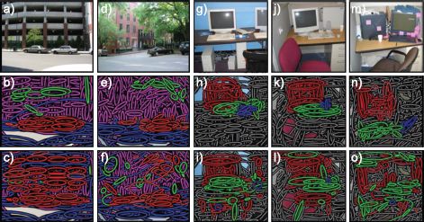
Figure 20.13 Scene recognition. a) Example street image. b) Results of scene parsing model. Each ellipse represents one word (i.e., the equivalent of the crosses in Figure 20.12). The ellipse color denotes the object label to which that word is assigned (part labels not shown). c) Results of the bag of words model, which makes elementary mistakes such as putting car labels at the top of the image as it has no spatial information. d) Another street scene. e) Interpretation with scene model and f) bag of words model. g-o) Three more office scenes parsed by the scene model and bag of words models. Adapted from Sudderth et al. (2008). ©2008 Springer.

20.7 Applications

In this chapter we have described a series of generative models for visual words of increasing complexity. Although these models are interesting, it should be emphasized that many applications use only the basic bag of words approach combined with a discriminative classifier. We now describe two representative examples of such systems.

20.7.1 Video Google

Sivic and Zisserman (2003) presented a system based on the bag of words, which can retrieve frames from a movie very efficiently based on a visual query; the user draws a bounding box around the object of interest and the system returns other images that contain the same object (Figure 20.14).

The system starts by identifying feature positions in each frame of the video. Unlike conventional bag of words models, these feature positions are tracked through several frames of video and rejected if this cannot be done. The averaged SIFT descriptor over each track is used to represent the image contents in the neighborhood of the feature. These descriptors are then clustered using K-means to create of the order of 6,000-10,000 possible visual words. Each feature is then assigned to one of these words based on the distance to the nearest cluster. Finally, each image or region is characterized by a vector containing the frequencies with which each visual word is found.

When the system receives a query, it compares the vector for the identified region to those for each potential region in the remaining video stream and retrieves those that are closest.

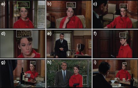
Figure 20.14 Video Google. a) The user identifies part of one frame of a video by drawing a bounding box around part of the scene. b-i) The system returns a ranked list of frames that contain the same object and identifies where it is in the image (white bounding boxes). The system correctly identifies the leopard-skin patterned hat in a variety of contexts despite changes in scale and position. In (h) it mistakes the texture of the vegetation in the background for an instance of the hat.

The implementation includes several features that make this process more reliable. First, it discards the top 5 percent and bottom 10 percent of words according to their frequency. This eliminates very common words that do not distinguish between frames and words that are very rare and are hence inefficient to search on. Second, it weights the distance measure using the term-frequency inverse document frequency scheme: the weight increases if the word is relatively rare in the database (the word is discriminative) and if it is used relatively frequently in this region (it is particularly representative of the region). Finally, the matches are considered more reliable if the spatial arrangement of visual words is similar. The final retrieved results are re-ranked based on their spatial consistency with the query.

The final system reliably returns plausible regions for a feature length movie in less than 0.1 seconds using an inverted file structure to facilitate efficient retrieval.

20.7.2 Action recognition

Laptev et al. (2008) applied a bag of words approach to action recognition in video sequences. They used a space-time extension of the Harris corner detector to find interest points in the video frames and extracted descriptors at multiple scales around each point. They eliminated detections at boundaries between shots.

To characterize the local motion and appearance, they computed histogram-based descriptors of the space time volumes surrounding these feature points. These were either based on the histogram of oriented gradients (HOG) descriptor (Section 13.3.3) or based on histograms of local motion. They clustered a subset of 100,000 descriptors from the training data using the K-means algorithm to create 4000 clusters and each feature in the test and training data was represented by the index of the nearest cluster center.

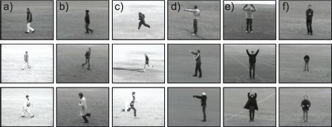
Figure 20.15 Example images from the KTH database (Schüldt et al. 2004). Images in (a-f) each show three examples of the six categories of walking, jogging, running, boxing, waving, and clapping, respectively. Using the bag of words approach of Laptev et al. (2008), these actions can be classified with over 90 percent accuracy.

They binned these quantized feature indices over a number of different space-time windows. The final decision about the action was based on a one-against-all binary classifier in which each action was separately considered and rated as being present or absent. The kernelized binary classifier combined information from the two different feature types and the different space time windows.

Laptev et al. (2008) first considered discriminating between six actions from the KTH database (Schüldt et al. 2004). This is a relatively simple dataset in which the camera is static and the action occurs against a relatively empty background (Figure 20.15). They discriminated between these classes with an average of 91.8 percent accuracy, with the major confusion being between jogging and running.

They also considered a more complex database containing eight different actions from movie sequences (Figure 20.16). It was notable that the performance here relied more on the HOG descriptors than the motion information, suggesting that the local context was providing considerable information (e.g., the action “get out of car” is more likely when a car is present). For this database, the performance was much worse, but it was significantly better than chance; action recognition “in the wild” is an open problem in computer vision research.

Discussion

The models in this chapter treat each image as a set of discrete features. The bag of features model, latent Dirichlet allocation, and single author-topic models do not explicitly describe the position of objects in the scene. Although they are effective for recognizing objects, they cannot locate them in the image. The constellation model improves this by allowing the parts of object to have spatial relations, and the scene model describes a scene as a collection of displaced parts.

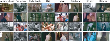
Figure 20.16 Action recognition in movie database of Laptev et al. (2008). a) Example true positives (correct detections), b) true negatives (action correctly identified as being absent), c) false positives (action classified as occurring but didn’t) d) false negatives (action classified as not occurring but did). This type of real-world action classification task is still considered very challenging.

Notes

Bag of words models: Sivic and Zisserman (2003) introduced the term “visual words” and first made the connection with text retrieval. Csurka et al. (2004) applied the bag of words methodology to object recognition. A number of other studies then exploited developments in the document search community. For example, Sivic et al. (2005) exploited probabilistic latent semantic analysis (Hofmann 1999) and latent Dirichlet allocation (Blei et al. 2003) for unsupervised learning of object classes. Sivic et al. (2008) extended this work to learn hierarchies of object classes. Li and Perona (2005) constructed a model very similar to the original author-topic model (Rosen-Zvi et al. 2004) for learning scene categories. Sudderth et al. (2005) and Sudderth et al. (2008) extended the author-topic model to contain information about the spatial layout of objects. The constellation and scene models presented in this chapter are somewhat simplified versions of this work. They also extended these models to cope with varying numbers of objects and or parts.

Applications of bag of words: Applications of the bag of words model include object recognition (Csurka et al. 2004), searching through video (Sivic and Zisserman 2003), scene recognition (Li and Perona 2005), and action recognition (Schüldt et al. 2004), and similar approaches have been applied to texture classfiication (Varma and Zisserman 2004) and labeling facial attributes (Aghajanian et al. 2009). Recent progress in object recognition can be reviewed by examining a recent summary of the PASCAL visual object classes challenge (Everingham et al. 2010). In the 2007 competition, bag of words approaches with no spatial information at all were still common. Several authors (Nistér and Stewénius 2006; Philbin et al. 2007; Jegou et al. 2008) have now presented large-scale demonstrations of object instance recognition based on bag of words, and this idea has been used in commercial applications such as “Google Goggles.”

Bag of words variants: Although we have discussed mainly generative models for visual words in this chapter, discriminative approaches generally yield somewhat better performance. Grauman and Darrell (2005) introduced the pyramid match kernel, which maps unordered data in a high-dimensional feature space into multiresolution histograms and computes a weighted histogram intersection in this space. This effectively performs the clustering and feature comparison steps simultaneously. This idea was extended to the spatial domain of the image itself by Lazebnik et al. (2006).

Improving the pipeline: Yang et al. (2007) and Zhang et al. (2007) provide quantitative comparisons showing how the various parts of the pipeline (e.g., the matching kernel, interest point detector, clustering method) affect object recognition results.

The focus of recent research has moved on to addressing various weaknesses of the pipeline such as the arbitrariness of the initial vector quantization step and the problem of regular patterns (Chum et al. 2007; Philbin et al. 2007, 2010; Jégou et al. 2009; Mikulik et al. 2010; Makadia 2010). The current trend is to increase the problem to realistic sizes and to this end new databases for object recognition (Deng et al. 2010) and scene recognition have been released (Xiao et al. 2010).

Action recognition: There has been a progression in recent years from testing action recognition algorithms in specially captured databases where the subject can easily be separated from the background (Schüldt et al. 2004), to movie footage (Laptev et al. 2008), and finally to completely unconstrained footage that may not be professionally shot and may have considerable camera shake. As this progression has taken place, the dominant approach has gradually become to base the system on visual words that capture the context of the scene as well as the action itself (Laptev et al. 2008). A comparison between approaches based on visual words and those that used explicit parts for action recognition in a still frame is presented by Delaitre et al. (2010). Recent work in this area has addressed unsupervised learning of action categories (Niebles et al. 2008).

Problems

20.1 The bag of words method in this chapter uses a generative approach to model the frequencies of the visual words. Develop a discriminative approach that models the probability of the object class as a function of the word frequencies.

20.2 Prove the relations in Equation 20.8, which show how to learn the latent Dirichlet allocation model in the case where we do know the part labels .

20.3 Show that the likelihood and prior terms are given by Equations 20.10 and 20.11, respectively.

20.4 Li and Perona (2005) developed an alternative model to the single author-topic model in which the hyperparameter α was different for each value of the object label w. Modify the graphical model for latent Dirichlet allocation to include this change.

20.5 Write out generative equations for the author-topic model in which multiple authors are allowed for each document. Draw the associated graphical model.

20.6 In real objects, we might expect visual words f that are adjacent to one another to take the same part label. How would you modify the author-topic model to encourage nearby part labels to be the same. How would the Gibbs sampling procedure for drawing samples from the posterior probability over parts be affected?

20.7 Draw a graphical model for the scene model described in Section 20.6.

20.8 All of the models in this chapter have dealt with classification; we wish to infer a discrete variable representing the state of the world based on discrete observed features {f_j}. Develop a generative model that can be used to infer a continuous variable based on discrete observed features (i.e., a regression model that uses visual words).

___________________________________

¹ More properly, we should define a prior over the mean and variance of the parts and marginalize over these parameters as well. This also avoids problems when no features are assigned to a certain part and hence the mean and covariance cannot be computed.