Computer Vision: Models, Learning, and Inference (2012)

This chapter concerns temporal models and tracking. The goal is to infer a sequence of world states {w_t}_t=1^T from a noisy sequence of measurements {x_t}_t=1^T. The world states are not independent; each is modeled as being contingent on the previous one. We exploit this statistical dependency to help estimate the state w_t even when the associated observation x_t is partially or completely uninformative.

Since the states form a chain, the resulting models are similar to those in Chapter 11. However, there are two major differences. First, in this chapter, we consider models where the world state is continuous rather than discrete. Second, the models here are designed for real-time applications; a judgment is made based on only the past and present measurements and without knowledge of those in the future.

A prototypical use of these temporal models is for contour tracking. Consider a parameterized model of an object contour (Figure 19.1). The goal is to track this contour through a sequence of images so that it remains firmly attached to the object. A good model should be able to cope with nonrigid deformations of the object, background clutter, blurring, and occasional occlusion.

19.1 Temporal estimation framework

Each model in this chapter consists of two components.

• The measurement model describes the relationship between the measurements x_t and the state w_t at time t. We treat this as generative, and model the likelihood Pr(x_t|w_t). We assume that the data at time t depend only on the state at time t and not those at any other time. In mathematical terms, we assume that x_t is conditionally independent of w_1…t−1 given w_t.

• The temporal model describes the relationship between states. Typically, we make the Markov assumption: we assume that each state depends only upon its predecessor. More formally, we assume that w_t is conditionally independent of the states w_1…t−2 given its immediate predecessor w_t−1, and just model the relationship Pr(w_t|w_t−1).

Together, these assumptions lead to the graphical model shown in Figure 19.2.

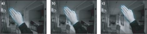
Figure 19.1 Contour tracking. The goal is to track the contour (solid blue line) through the sequence of images so that it remains firmly attached to the object (see Chapter 17 for more information about contour models). The estimation of the contour parameters is based on a temporal model relating nearby frames, and local measurements from the image (e.g., between the dashed blue lines). Adapted from Blake and Isard (1998). ©1998 Springer.

19.1.1 Inference

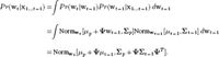
In inference, the general problem is to compute the marginal posterior distribution Pr(w_t|x_1…t) over the world state w_t at time t, given all of the measurements x_1…t up until this time. At time t = 1, we have only observed a single measurement x₁, so our prediction is based entirely on this datum. To compute the posterior distribution Pr(w₁|x₁), Bayes’ rule is applied:

where the distribution Pr(w₁) contains our prior knowledge about the initial state.

At time t = 2 we observe a second measurement x₂. We now aim to compute the posterior distribution of the state at time t = 2 based on both x₁ and x₂. Again, we apply Bayes’ rule,

Notice that the likelihood term Pr(x₂|w₂) is only dependent on the current measurement x₂ (according to the assumption stated earlier). The prior Pr(w₂|x₁) is now based on what we have learned from the previous measurement; the possible values of the state at this time depend on our knowledge of what happened at the previous time and how these are affected by the temporal model.

Generalizing this procedure to time t, we have

To evaluate this, we must compute Pr(w_t|x_1…t−1), which represents our prior knowledge about w_t before we look at the associated measurement x_t. This prior depends on our knowledge Pr(w_t−1|x_1…t−1) of the state at the previous time and the temporal model Pr(w_t|w_t−1), and is computed recursively as

which is known as the Chapman-Kolmogorov relation. The first term in the integral represents the prediction for the state at time t given a known state w_t−1 at time t−1. The second term represents the uncertainty about what the state actually was at time t−1. The Chapman-Kolmogorov equation amalgamates these two pieces of information to predict what will happen at time t.

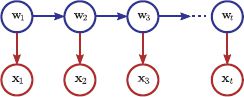
Figure 19.2 Graphical model for Kalman filter and other temporal models in this chapter. This implies the following conditional independence relation: the state w_t is conditionally independent of the states w_1…t−2 and the measurements x_1…t−1 given the previous state w_t−1.

Hence, inference consists of two alternating steps. In the prediction step, we compute the prior Pr(w_t|x_1…t−1) using the Chapman-Kolmogorov relation (Equation 19.4). In the measurement incorporation step, we combine this prior with the new information from the measurement x_t using Bayes’s rule (Equation 19.3).

19.1.2 Learning

The goal of learning is to estimate the parameters θ that determine the relationship Pr(w_t|w_t−1) between adjacent states and the relationship Pr(x_t|w_t) between the state and the data, based on several observed time sequences.

If we know the states for these sequences, then this can be achieved using the maximum likelihood method. If the states are unknown, then they can be treated as hidden variables, and the model can be learned using the EM algorithm (Section 7.8). In the E-step, we compute the posterior distribution over the states for each time sequence. This is a process similar to the inference method described earlier, except that it also uses data from later in the sequence (Section 19.2.6). In the M-step, we update the EM bound with respect to θ.

The rest of this chapter focusses on inference in this type of temporal model. We will first consider the Kalman filter. Here the uncertainty over the world state is described by a normal distribution,¹ the relationship between the measurements and the world is linear with additive normal noise, and the relationship between the state at adjacent times is also linear with additive normal noise.

19.2 Kalman filter

To define the Kalman filter, we must specify the temporal and measurement models. The temporal model relates the states at times t − 1 and t and is given by

where μ_p is a D_w × 1 vector, which represents the mean change in the state, and Ψ is a D_w × D_w matrix, which relates the mean of the state at time t to the state at time t−1. This is known as the transition matrix. The term ∊_p is a realization of the transition noise, which is normally distributed with covariance ∑_p and determines how closely related the states are at times t and t−1. Alternately, we can write this in probabilistic form:

The measurement model relates the data x_t at time t to the state w_t,

where μ_m is a D_x × 1 mean vector and Φ is a D_x × D_w matrix relating the D_x × 1 measurement vector to the D_w × 1 state. The term ∊_m is a realization of the measurement noise that is normally distributed with covariance ∑_m. In probabilistic notation, we have

Notice that the measurement equation is identical to the relation between the data and the hidden variable in the factor analysis model (Section 7.6); here the state w replaces the hidden variable h. In the context of the Kalman filter, the dimension D_w of the state w is often larger than the dimension D_x of the measurements x, so Φ is a landscape matrix, and the measurement noise ∑_m is not necessarily diagonal.

The form of both the temporal and measurement equations is the same: each is a normal probability distribution where the mean is a linear function of another variable and the variance is constant. This form has been carefully chosen because it ensures that if the marginal posterior Pr(w_t−1|x_1…t−1) at time t−1 was normal, then so is the marginal posterior Pr(w_t|x_1…t) at time t. Hence, the inference procedure consists of a recursive updating of the means and variances of these normal distributions. We now elaborate on this procedure.

19.2.1 Inference

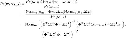
In inference, the goal is to compute the posterior probability Pr(w_t|x_1…t) over the state w_t given all of the measurements x_1…t so far. As before, we apply the prediction and measurement-incorporation steps to recursively estimate Pr(w_t|x_1…t) from Pr(w_t−1|x_1…t−1). The latter distribution is assumed to be normal with mean μ_t−1 and variance ∑_t−1.

In the prediction step, we compute the prior at time t using the Chapman-Kolmogorov equation

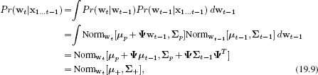
where we have denoted the predicted mean and variance of the state by μ₊ and ∑₊. The integral between lines 2 and 3 was solved by using Equations 5.17 and 5.14 to rewrite the integrand as proportional to a normal distribution in w_t−1. Since the integral of any pdf is one, the result is the constant of proportionality, which is itself a normal distribution in w_t.

In the measurement incorporation step, we apply Bayes’ rule,

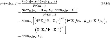
where we have used Equation 5.17 on the likelihood term and then combined the likelihood and prior using Equation 5.14. The right-hand side is now proportional to a normal distribution in w_t, and the constant of proportionality must be one to ensure that the posterior on the left-hand side is a valid distribution.

Notice that the posterior Pr(w_t|x_1…t) is normal with mean μ_t and covariance ∑_t. We are in the same situation as at the start, so the procedure can be repeated for the next time step.

It can be shown that the mean of the posterior is a weighted sum of the values predicted by the measurements and the prior knowledge, and the covariance is smaller than either. However, this is not particularly obvious from the equations. In the following section we rewrite the equation for the posterior in a form that makes these properties more obvious.

19.2.2 Rewriting measurement incorporation step

The measurement incorporation step is rarely presented in the above form in practice. One reason for this is that the equations for μ_t and ∑_t contain an inversion that is of size D_w × D_w. If the world state is much higher dimensional than the observed data, then it would be more efficient to reformulate this as an inverse of size D_x × D_x. To this end, we define the Kalman gain as

We will use this to modify the expressions for μ_t and ∑_t from Equation 19.10. Starting with μ_t, we apply the matrix inversion lemma (Appendix C.8.4):

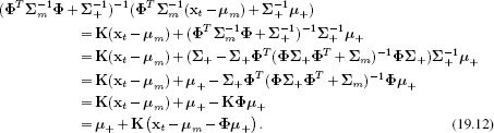
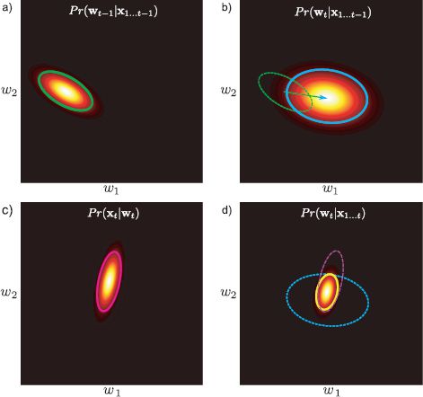
Figure 19.3 Recursive inference in the Kalman filter. a) The posterior probability Pr(w_t−1|x_1…t−1) of the state w_t−1 given all of the measurements x_1…t−1 up to that time takes the form of a normal distribution (green ellipse). b) In the prediction step, we apply the Chapman-Kolmogorov relation to estimate the prior Pr(w_t|x_1…t−1), which is also a normal distribution (cyan ellipse). c) The measurement likelihood Pr(x_t|w_t) is proportional to a normal distribution (magenta ellipse). d) To compute the posterior probability Pr(w_t|x_1…t), we apply Bayes’ rule by taking the product of the prior from panel (b) and the likelihood from panel (c) and normalizing. This yields a new normal distribution (yellow ellipse) and the procedure can begin anew.

The expression in brackets in the final line is known as the innovation and is the difference between the actual measurements x_t and the predicted measurements μ_m + Φ μ₊ based on the prior estimate of the state. It is easy to see why K is termed the Kalman gain: it determines the amount that the measurements contribute to the new estimate in each direction in state space. If the Kalman gain is small in a given direction, then this implies that the measurements are unreliable relative to the prior and should not influence the mean of the state too much. If the Kalman gain is large in a given direction, then this suggests that the measurements are more reliable than the prior and should be weighted more highly.

We now return to the covariance term of Equation 19.10. Using the matrix inversion lemma, we get

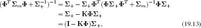
which also has a clear interpretation: the posterior covariance is equal to the prior covariance less a term that depends on the Kalman gain: we are always more certain about the state after incorporating information due to the measurement, and the Kalman gain modifies how much more certain we are. When the measurements are more reliable, the Kalman gain is high, and the covariance decreases more.

After these manipulations, we can rewrite Equation 19.10 as

19.2.3 Inference summary

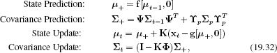
Developing the inference equations was rather long-winded, so here we summarize the inference process in the Kalman filter (see also Figure 19.3). We aim to compute the marginal posterior probability Pr(w_t|x_1…t) based on a normally distributed estimate of the marginal posterior probability Pr(w_t−1|x_1…t−1) at the previous time and a new measurement x_t. If the posterior probability at time t − 1 has mean μ_t−1 and variance ∑_t−1, then the Kalman filter updates take the form

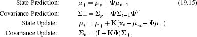
where

In the absence of prior information at time t = 1, it is usual to initialize the prior mean μ₀ to any reasonable value and the covariance ∑₀ to a large multiple of the identity matrix representing our lack of knowledge.

19.2.4 Example 1

The Kalman filter update equations are not very intuitive. To help understand the properties of this model, we present two toy examples. In the first case, we consider an object that is approximately circling a central point in two dimensions. The state consists of the two-dimensional position of the object. The actual set of states can be seen in Figure 19.4a.

Let us assume that we do not have a good temporal model that describes this motion. Instead, we will assume the simplest possible model. The Brownian motion model assumes that the state at time t+1 is similar to the state at time t:

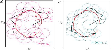
Figure 19.4 Kalman filter example 1. The true state (red dots) evolves in a 2D circle. The measurements (magenta dots) consist of direct noisy observations of the state. a) Posterior probability Pr(w_t|x_t) of state using measurements alone (uniform prior assumed). The mean of each distribution is centered on the associated datapoint, and the covariance depends on the measurement noise. b) Posterior probabilities based on Kalman filter. Here the temporal equation describes the state as a random perturbation of the previous state. Although this is not a good model (the circular movement is not accounted for), the posterior covariances (blue ellipses) are smaller than without the Kalman filter (magenta ellipses in (a)) and the posterior means (blue dots) are closer to the true states (red dots) than the estimates due to the measurements alone (magenta dots in (a)).

This is a special case of the more general formulation in Equation 19.6. Notice that this model has no insight into the fact that the object is rotating.

For ease of visualization, we will assume that the observations are just noisy realizations of the true 2D state so that

where ∑_m is diagonal. This is a special case of the general formulation in 19.8.

In inference, the goal is to estimate the posterior probability over the state at each time step given the observed sequence so far. Figure b shows the sequence of posterior probabilities Pr(w_t|x_1…t) over the state after running the Kalman recursions. It is now easy to understand why this is referred to as the Kalman filter: the MAP states (the peaks of the marginal posteriors) are smoothed relative to estimates from the measurements alone. Notice that the Kalman filter estimate has a lower covariance than the estimate due to the measurements alone (Figure 19.4a). In this example, the inclusion of the temporal model makes the estimates both more accurate and more certain, even though the particular choice of temporal model is wrong.

19.2.5 Example 2

Figure 19.5 shows a second example where the setup is the same except that the observation equation differs at alternate time steps. At even time steps, we observe a noisy estimate of just the first dimension of the state w. At odd time steps, we observe only a noisy estimate of the second dimension. The measurement equations are

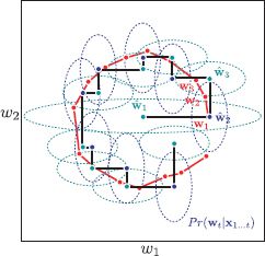
Figure 19.5 Kalman filter example 2. As for example 1, the true state (red points) proceeds in an approximate circle. We don’t have access to this temporal model and just assume that the new state is a perturbation of the previous state. At even time steps, the measurement is a noisy realization of the first dimension (horizontal coordinate) of the state. At odd time steps, it is a noisy realization of the second dimension (vertical coordinate). The Kalman filter produces plausible estimates (blue and cyan points and ellipses) even though a single measurement is being used to determine a 2D state at any time step.

This is an example of a nonstationary model: the model changes over time.

We use the same set of ground truth 2D states as for example 1 and simulate the associated measurements using Equation 19.19. The posterior probability over the state was computed using the Kalman filter recursions with the relevant measurement matrix Φ at each time step.

The results (Figure 19.5) show that the Kalman filter maintains a good estimate of the 2D state despite having only a 1D measurement at each time step. At odd time steps, the variance in the first dimension decreases (due to the information from the measurement), but the variance in the second dimension increases (due to the uncertainty in the temporal model). At even time steps, the opposite occurs.

This model may seem esoteric, but it is common in many imaging modalities for different aspects of the measurements to arrive at different times. One option is to wait until a full set of measurements is present before estimating the state, but this means that many of them are out of date. Incorporation of each measurement when it arrives using a Kalman filter is a superior approach.

19.2.6 Smoothing

The preceding inference procedure is designed for real-time applications where the estimation of the state is based only on measurements from the past and present. However, there may be occasions where we wish to infer the state using measurements that lie in the future. In the parlance of Kalman filters, this is known as smoothing.

We consider two cases. The fixed lag smoother is still intended for on-line estimation, but it delays the decision about the state by a fixed number of time steps. The fixed interval smoother assumes that we have observed all of the measurements in the entire sequence before we make a judgment about the world state.

Fixed lag smoother

The fixed lag smoother relies on a simple trick. To estimate the state delayed by τ time steps, we augment the state vector to contain the delayed estimates of the previous τ times. The time update equation now takes the form

where the notation w_t^[m] refers to the state at time t − m based on measurements up to time t, and w_t^[τ] is the quantity we wish to estimate. This state evolution equation clearly fits the general form of the Kalman filter (Equation 19.5). It can be parsed as follows: in the first equation of this system, the temporal model is applied to the current estimate of the state. In the remaining equations, the delayed states are created by simply copying the previous state.

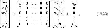
The associated measurement equation is

which fits the form of the Kalman filter measurement model (Equation 19.7). The current measurements are based on the current state, and the time-delayed versions play no part. Applying the Kalman recursions with these equations computes not just the current estimate of the state but also the time-delayed estimates.

Fixed interval smoother

The fixed interval smoother consists of a backward set of recursions that estimate the marginal posterior distributions Pr(w_t|x_1…T) of the state at each time step, taking into account all of the measurements x_1…T. In these recursions, the marginal posterior distribution Pr(w_t|x_1…T) of the state at time t is updated. Based on this result, the marginal posterior Pr(w_t−1|x_1…T) at time t−1 is updated and so on. We denote the mean and variance of the marginal posteriorPr(w_t|x_1…T) at time t by μ_t|T and ∑_t|T, respectively, and use

where μ_t and ∑_t are the estimates of the mean and covariance from the forward pass. The notation μ_+|t and ∑_+|t denotes the mean and variance of the posterior distribution Pr(w_t|x_1…t−1) of the state at time t based on the measurements up to time t−1 (i.e., what we denoted as μ₊ and ∑₊ during the forward Kalman filter recursions) and

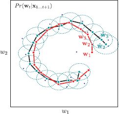
Figure 19.6 Fixed lag Kalman smoothing. The estimated state (light blue dots) and the associated covariance (light blue ellipses) were estimated using a lag of 1 time step: each estimate is based on all of the data in the past, the present observation and the observation one step into the future. The resulting estimated states have a smaller variance than for the standard Kalman filter (Compare to Figure 19.4b) and are closer to the true state (red dots). In effect, the estimate averages out the noise in the measurements (dark blue dots). The cost of this improvement is that there is a delay of one time step.

It can be shown that the backward recursions correspond to the backward pass of sum-product belief propagation in the Kalman filter graphical model.

19.2.7 Temporal and measurement models

The choice of temporal model in the Kalman filter is restricted to be linear and is dictated by the matrix Ψ. Despite this limitation, it is possible to build a surprisingly versatile family of models within this framework. In this section we review a few of the best-known examples.

1. Brownian motion: The simplest model is Brownian motion Figure 19.7a in which the state is operated upon by the identity matrix so that

2. Geometric transformations: The family of linear filters includes geometric transformations such as rotations, stretches, and shears. For example, choosing Ψ so that Ψ^T Ψ = I and |Ψ| = 1 creates a rotation around the origin Figure 19.7b: this is the true temporal model in Figures 19.4-19.6.

3. Velocities and accelerations: The Brownian motion model can be extended by adding a constant velocity v to the motion model (Figure 19.7c) so that.

To incorporate a changing velocity, we can enhance the state vector to include the velocity term so that

This has the natural interpretation that the velocity term contributes an offset to the state at each time. However, the velocity is itself uncertain and is related by a Brownian motion model to the velocity at the previous time step. For the measurement equation, we have

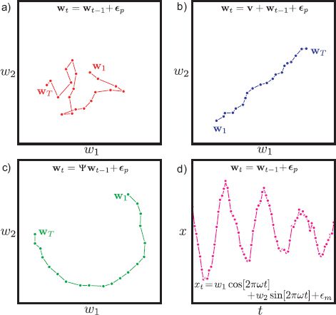
Figure 19.7 Temporal and measurement models. a) Brownian motion model. At each time step the state is randomly perturbed from the previous position, so a drunken walk through state space occurs. b) Constant velocity model. At each time step, a constant velocity is applied in addition to the noise. c) Transformation model. At each time step, the state is rotated about the origin and noise is added. d) Oscillatory measurements. These quasi-sinusoidal measurements are created from a two-dimensional state that itself undergoes Brownian motion. The two elements of the state control the sinusoidal and co-sinusoidal parts of the measurements.

In other words, the measurements at time t do not directly depend on the velocity term, only the state itself. This idea can be easily extended to include an acceleration term as well.

4. Oscillatory data: Some data are naturally oscillatory. To describe oscillatory 1D data, we could use a state containing a 2 × 1 state vector w using Brownian motion as the temporal model. We then implement the nonstationary measurement equation

For a fixed state w, this model produces noisy sinusoidal data. As the state varies due to the Brownian motion of the temporal model, the phase and amplitude of the quasi-sinusoidal output will change (19.7d).

19.2.8 Problems with the Kalman filter

Although the Kalman filter is a flexible tool, it has a number of shortcomings (Figure 19.8). Most notably,

• It requires the temporal and measurement equations to be linear, and

• It assumes that the marginal posterior is unimodal and can be well captured by a mean and covariance; hence, it can only ever have one hypothesis about the position of the object.

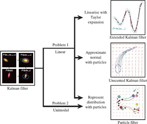
Figure 19.8 Temporal models for tracking. The Kalman filter has two main problems: first, it requires the temporal and measurement models to be linear. This problem is directly addressed by the extended and unscented Kalman filters. Second, it represents the uncertainty with a normal distribution that is uni-modal and so cannot maintain multiple hypotheses about the state. This problem is tackled by particle filters.

In the following sections, we discuss models that address these problems. The extended Kalman filter and the unscented Kalman filter both allow nonlinear state update and measurement equations. Particle filtering abandons the use of the normal distribution and describes the state as a complex multimodal distribution.

19.3 Extended Kalman filter

The extended Kalman filter (EKF) is designed to cope with more general temporal models, where the relationship between the states at time t is an arbitrary nonlinear function f[•,•] of the state at the previous time step and a stochastic contribution ∊_p

where the covariance of the noise term ∊_p is ∑_p as before. Similarly, it can cope with a nonlinear relationship g[•,•] between the state and the measurements

where the covariance of ∊_m is ∑_m.

The extended Kalman filter works by taking linear approximations to the nonlinear functions at the peak μ_t of the current estimate using the Taylor expansion. If the function is not too nonlinear, then this approximation will adequately represent the function in the region of the current estimate and we can proceed as usual. We define the Jacobian matrices,

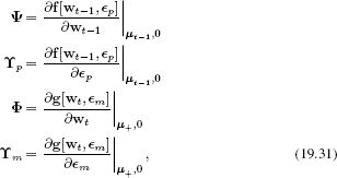
where the notation |_μ+,0 denotes that the derivative is computed at position w = μ₊ and ∊ = 0. Note that we have overloaded the meaning of Φ and Ψ here. Previously they represented the linear transformations between states at adjacent times, and between the state and the measurements, respectively. Now they represent the local linear approximation of the nonlinear functions relating these quantities.

The update equations for the extended Kalman filter are

where

In the context of fixed interval smoothing, the results can be improved by performing several passes back and forth through the data, relinearizing around the previous estimates of the state in each sweep. This is called the iterated extended Kalman filter.

In conclusion, the extended Kalman filter is conceptually simple, but only copes with relatively benign nonlinearities. It is a heuristic solution to the nonlinear tracking problem and may diverge from the true solution.

19.3.1 Example

Figure 19.9 shows a worked example of the extended Kalman filter. In this case, the time update model is nonlinear, but the observation model is still linear:

where ∊_p is a normal noise term with covariance ∑_p, ∊_m is a normal noise term with covariance ∑_m, and the nonlinear function f[•,•] is given by

The Jacobian matrices for this model are easily computed. The matrices _p, Φ, and _m are all equal to the identity. The Jacobian matrix Ψ is

The results of using this system for tracking are illustrated in Figure 19.9. The extended Kalman filter successfully tracks this nonlinear model giving results that are both closer to the true state and more confident than estimates based on the individual measurements alone. The EKF works well here because the nonlinear function is smooth and departs from linearity slowly relative to the time steps: consequently, the linear approximation is reasonable.

19.4 Unscented Kalman filter

The extended Kalman filter is only reliable if the linear approximations to the functions f[•,•] or g[•,•] describe them well in the region of the current position. Figure 19.10 shows a situation where the local properties of the temporal function are not representative and so the EKF estimate of the covariance is inaccurate.

The unscented Kalman filter (UKF) is a derivative-free approach that partially circumvents this problem. It is suited to nonlinear models with additive normally distributed noise so that the temporal and measurement equations are

To understand how the UKF works, consider a nonlinear temporal model. Given the mean and covariance of the normally distributed posterior distribution Pr(w_t−1|x_1…t−1) over the state at time t−1, we wish to predict a normally distributed prior Pr(w_t|x_1…t−1) over the state at time t. We proceed by

• Approximating the normally distributed posterior Pr(w_t−1|x_1…t−1) with a set of point masses that are deterministically chosen so that they have the same mean μ_t−1 and covariance ∑_t−1 as the original distribution,

• Passing each of the point masses through the nonlinear function, and then

• Setting the predicted distribution Pr(w_t|x_1…t−1) at time t to be a normal distribution with the mean and covariance of the transformed point masses.

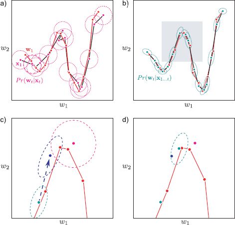
Figure 19.9 The extended Kalman filter. a) The temporal model that transforms the state (red dots) here is nonlinear. Each observed data point (magenta dots) is a noisy copy of the state at that time. Based on the data alone, the posterior probability over the state is given by the magenta ellipses. b) Estimated marginal posterior distributions using the extended Kalman filter: the estimates are more certain and more accurate than using the measurements alone. c) Close-up of shaded region from (b). The EKF makes a normal prediction (dark blue ellipse) based on the previous state (light blue ellipse) and the linearized motion model. The measurement makes a different prediction (magenta ellipse). d) The EKF combines these two predictions to get an improved estimate (light blue ellipse).

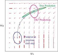
Figure 19.10 Problems with the EKF. A 2D temporal function f[•,•] operates on the state (red lines indicate gradient direction). In the prediction step, the previous estimate (blue ellipse) should be passed through this function (to create distorted green ellipse) and noise added (not shown). The EKF approximates this by passing the mean through the function and updating the covariance based on a linear approximation of the function at the previous state estimate. Here, the function changes quite nonlinearly, and so this approximation is bad, and the predicted covariance (magenta ellipse) is inaccurate.

This process is illustrated in Figure 19.11.

As for the extended Kalman filter, the predicted state Pr(w_t|x_1…t−1) in the UKF is a normal distribution. However, this normal distribution is a provably better approximation to the true distribution than that provided by the EKF. A similar approach is applied to cope with a nonlinearity in the measurement equations. We will now consider each of these steps in more detail.

19.4.1 State evolution

As for the standard Kalman filter, the goal of the state evolution step is to form a prediction Pr(w_t|x_1…t−1) about the state at time t by applying the temporal model to the posterior distribution Pr(w_t−1|x_1…t−1) at the previous time step. This posterior distribution is normal with mean μ_t−1 and covariance ∑_t−1, and the prediction will also be normal with mean μ₊ and covariance ∑₊.

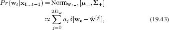
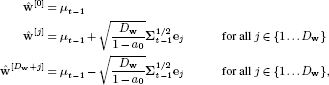
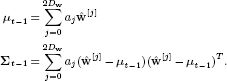
We proceed as follows. We approximate the marginal posterior at the previous time step by a weighted sum of 2D_w+1 delta functions, where D_w is the dimensionality of the state, so that

where the weights {a_j}_j=0^2D_w are positive and sum to one. In this context, the delta functions are referred to as sigma points. The positions {^[j]}^2D_wj=0 of the sigma points are carefully chosen so that

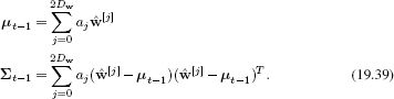
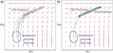
Figure 19.11 Temporal update for unscented Kalman filter. a) In the temporal update step, the posterior distribution from the previous time step (which is a normal) is approximated by a weighted set of point masses that collectively have the same mean and covariance as this normal. Each of these is passed through the temporal model (dashed lines). A normal prediction is formed by estimating the mean and the covariance of the transformed point masses. In a real system, the variance would subsequently be inflated to account for additive uncertainty in the position. b) The resulting prediction is quite close to the true prediction and for this case is much better than that of the extended Kalman filter (see Figure 19.10).

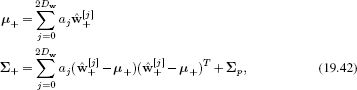
One possible scheme is to choose sigma points

where e_j is the unit vector in the j^th direction. The associated weights are chosen so that a₀ ∈ [0,1] and

for all a_j. The choice of weight a₀ of the first sigma point determines how far the remaining sigma points are from the mean.

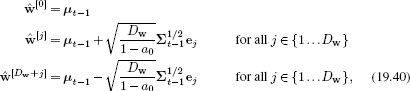
We pass the sigma points through the nonlinearity, to create a new set of samples ₊^[j] = f[^[j]] that collectively form a prediction for the state. We then compute the mean and the variance of the predicted distribution Pr(w_t|x_1…t−1) from the mean and variance of the transformed points so that

where we have added an extra term Σ_p to the predicted covariance to account for the additive noise in the temporal model.

19.4.2 Measurement incorporation

The measurement incorporation process in the UKF uses a similar idea: we approximate the predicted distribution Pr(w_t|x_1…t−1) as a set of delta functions or sigma points

where we choose the centers of the sigma points and the weights so that

For example, we could use the scheme outlined in Equations 19.40 and 19.41.

Then the sigma points are passed through the measurement model ^[j] = g[^[j]] to create a new set of points {^[j]}^2D_wj=0 in the measurement space. We compute the mean and covariance of these predicted measurements using the relations

The measurement incorporation equations are now

where the Kalman gain K is now redefined as

As for the prediction step, it can be shown that the UKF approximation is better than that of the EKF.

19.5 Particle filtering

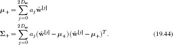
The extended and unscented Kalman filters can partially cope with nonlinear temporal and measurement models. However, they both represent the uncertainty over the state as a normal distribution. They are hence ill-equipped to deal with situations where the true probability distribution over the state is multimodal. Figure 19.12 illustrates a temporal model that maps nearby states into two distinct regions. In this situation, neither the EKF nor the UKF suffice: the EKF models only one of the resulting clusters and the UKF tries to model both with a single normal model, assigning a large probability to the empty region between the clusters.

Figure 19.12 The need for particle filtering. a) Consider this new temporal update function (change of state with time indicated by red pointers), which bifurcates around the horizontal midline. b) With the EKF, the predicted distribution after the time update is toward the bottom, as the initial mean was below the bifurcation. The linear approximation is not good here and so the covariance estimate is inaccurate. c) In the UKF, one of the sigma points that approximates the prior is above the midline and so it is moved upward (green dashed line), whereas the others are below the midline and are moved downward (other dashed lines). The estimated covariance is very large. d) We can get an idea of the true predicted distribution by sampling the posterior at the previous time step and passing the samples through the nonlinear temporal model. It is clear that the resulting distribution is bimodal and can never be well approximated with a normal distribution. The particle filter represents the distribution in terms of particles throughout the tracking process and so it can describe multimodal distributions like this.

Particle filtering resolves this problem by representing the probability density as a set of particles in the state space. Each particle can be thought of as representing a hypothesis about the possible state. When the state is tightly constrained by the data, all of these particles will lie close to one another. In more ambiguous cases, they will be widely distributed or clustered into groups of competing hypotheses.

The particles can be evolved through time or projected down to simulate measurements regardless of how nonlinear the functions are. The latter exercise leads us to another nice property of the particle filter: since the state is multimodal, so are the predicted measurements. In turn, the measurement density may also be multimodal. In vision systems, this means that the system copes much better with clutter in the scene (Figure 19.14). As long as some of the predicted measurements agree with the measurement density, the tracker should remain stable.

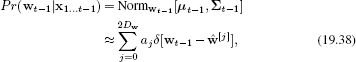
One of the simplest particle filter methods is the conditional density propagation or condensation algorithm. The probability distribution Pr(w_t−1|x_1…t−1) is represented by a weighted sum of J weighted particles:

where the weights are positive and sum to one. Each particle represents a hypothesis about the state and the weight of the particle indicates our confidence in that hypothesis. Our goal is to compute the probability distribution Pr(w_t|x_1…t) at the next time step, which will be represented in a similar fashion. As usual this process is divided into a time evolution and a measurement incorporation step, which we now consider in turn.

19.5.1 Time evolution

In the time evolution step, we create J predictions ^[j]₊ for the time-evolved state. Each is represented by an unweighted particle. We create each prediction by re-sampling so that we

• choose an index n ∈ {1…J} of the original weighted particles where the probability is according to the weights. In other words, we draw a sample from Cat_n[a] and

• draw the sample ^[j]₊ from the temporal update distribution Pr(w_t|w_t−1 = ^[n]_t−1) (Equation 19.37).

In this process, the final unweighted particles ^[j]₊ are created from the original weighted particles ^[j]_t−1 according to the weights a=[a₁,a₂,…,a_J]. Hence, the highest weighted original particles may contribute repeatedly to the final set, and the lowest weighted ones may not contribute at all.

19.5.2 Measurement incorporation

In the measurement incorporation step we weight the new set of particles according to how well they agree with the observed data. To this end, we

• Pass the particles through the measurement model ^[j]₊ = g[^[j]₊].

• Weight the particles according to their agreement with the observation density. For example, with a Gaussian measurement model, we could use

• Normalize the resulting weights {a_j}^J_j=1 to sum to one.

• Finally, set the new states ^[j]_t to the predicted states ^[j]₊ and the new weights to a_j.

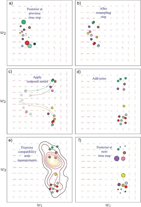
Figure 19.13 The condensation algorithm. a) The posterior at the previous step is represented as a set of weighted particles. b) The particles are re-sampled according to their weights to produce a new set of unweighted particles. c) These particles are passed through the nonlinear temporal function. d) Noise is added according to the temporal model. e) The particles are passed through the measurement model and compared to the measurement density. f) The particles are reweighted according to their compatibility with the measurements, and the process can begin again.

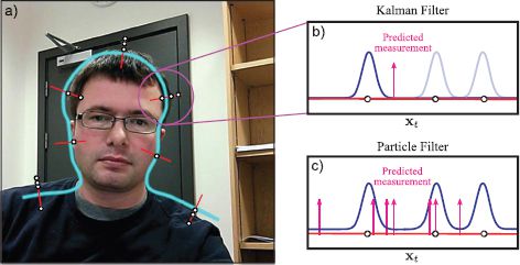
Figure 19.14 Data association. a) Consider the problem of tracking this contour. The contour from the previous frame is shown in cyan, and the problem is to incorporate the measurements in this frame. These measurements take the form of edges along one-dimensional slices perpendicular to the contour. In most cases, there are multiple possible edges that might be due to the contour. b) In the Kalman filter, the measurement density is constrained to be normal: we are forced to choose between the different possible hypotheses. A sensible way to do this is to select the one that is closest to the predicted measurement. This is known as data association. c) In the particle filter, there are multiple predicted measurements and it is not necessary that the measurement density is normal. We can effectively take into account all of the possible measurements.

Figure 19.13 demonstrates the action of the particle filter. The filter copes elegantly with the multimodal probability distribution. It is also suitable for situations where it is not obvious which aspect of the data is the true measurement. This is known as the data association problem (Figure 19.14).

The main disadvantage of particle filters is their cost: in high dimensions, a very large number of particles may be required to get an accurate representation of the true distribution over the state.

19.5.3 Extensions

There are many variations and extensions to the particle filter. In many schemes, the particles are not resampled on each iteration, but only occasionally so the main scheme operates with weighted particles. The resampling process can also be improved by applying importance sampling. Here, the new samples are generated in concert with the measurement process, so that particles that agree with the measurements are more likely to be produced. This helps prevent the situation where none of the unweighted samples after the prediction stage agree with the measurements.

The process of Rao-Blackwellization partitions the state into two subsets of variables. The first subset is tracked using a particle filter, but the other subset is conditioned on the first subset and evaluated analytically using a process more like the Kalman filter. Careful choice of these subsets can result in a tracking algorithm that is both efficient and accurate.

19.6 Applications

Tracking algorithms can be used in combination with any model that is being reestimated over a time sequence. For example, they are often used in combination with 3D body models to track the pose of a person in video footage. In this section, we will describe three example applications. First we will consider tracking the 3D position of a pedestrian in a scene. Second, we will describe simultaneous localization and mapping (SLAM) in which both a 3D representation of a scene and the pose of the camera viewing it are estimated through a time sequence. Finally, we will consider contour tracking for an object with complex motion against a cluttered background.

19.6.1 Pedestrian Tracking

Rosales and Sclaroff (1999) described a system to track pedestrians in 2D from a fixed static camera using the extended Kalman filter. For each frame, the measurements x consisted of a 2D bounding box x = {x₁, y₁, x₂, y₂} around the pedestrian. This was found by segmenting the pedestrian from the background using a background subtraction model, and finding a connected region of foreground pixels.

The state of the world w was considered to be the 3D position of a bounding box of constant depth {u₁, v₁, u₂, v₂, w} and the velocities associated with these five quantities. The state update equation assumed first-order Newtonian dynamics in 3D space. The relationship between the state and measurements was

which mimics the nonlinear action of the pinhole camera.

Results from the tracking procedure are illustrated in Figure 19.15. The system successfully tracks pedestrians and was extended to cope with occlusions (which are predicted by the EKF based on the estimated trajectory of the objects). In the full system, the estimated bounding boxes are used to warp the images of the pedestrians to a fixed size, and the resulting registered images were used as input to an action recognition algorithm

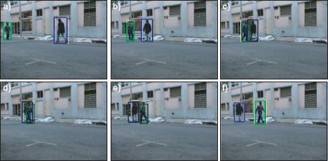
Figure 19.15 Pedestrian tracking results. a-f) Six frames from a sequence in which a 3D bounding plane of constant depth was used to track each person. Adapted from Rosales and Sclaroff (1999). © 1999 IEEE.

19.6.2 Monocular SLAM

The goal of simultaneous localization and mapping or SLAM is to build a map of an unknown environment based on measurements from a moving sensor (usually attached to a robot) and to establish where the sensor is in the world at any given time. Hence, the system must simultaneously estimate the structure of the world and its own position and orientation within that model. SLAM was originally based on range sensors but in the last decade it has become possible to build systems based on a monocular camera that work in real time. In essence it is a real-time version of the sparse 3D reconstruction algorithms discussed in Chapter 16.

Davison et al. (2007) presented one such system which was based on the extended Kalman filter. Here the world state w contains

• The camera position (u, v, w),

• The orientation of the camera as represented by a 4D quaternion q,

• The velocity and angular velocity, and

• A set of 3D points {p_k} where p_k = [p_uk,p_vk,p_wk]. This set generally expands during the sequence as more parts of the world are seen.

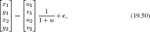
The state update equation modifies the position and orientation according to their respective velocities, and allows these velocities themselves to change. The observation equation maps each 3D point through a pinhole camera model to create a predicted 2D image position (i.e., similar to Equation 19.50). The actual measurements consist of interest points in the image, which are uniquely identified and associated with the predicted measurements by considering their surrounding region. The system is very efficient as it is only necessary to search the image in regions close to the 2D point predicted by the measurement equation from the current state.

The full system is more complex, and includes special procedures for initializing new feature points, modeling the local region of each point as a plane, selecting which features to measure in this frame, and managing the resulting map by deleting extraneous features to reduce the complexity. A series of frames from the system is illustrated in Figure 19.16.

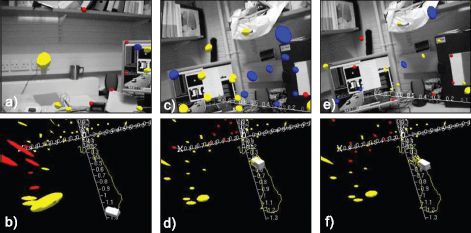
Figure 19.16 Monocular SLAM model of Davison et al. (2007). a) Current view of world with visual features and their 3D covariance ellipse superimposed. Yellow points are features in the model that were actually measured. Blue points are features in the model that were not detected in this frame. Red points are new features that can potentially be incorporated into the model. b) Model of world at the time this frame was captured, showing the position of the camera and the position and uncertainty of visual features. c-f) Two more pairs of images and associated models from later in the same time sequence. Notice that the uncertainty in the feature positions gradually decreases over time. Adapted from Davison et al. (2007). ©2007 IEEE.

19.6.3 Tracking a contour through clutter

In Section 17.3 we discussed fitting a template shape model to an image. It was noted that this was a challenging problem as the template frequently fell into local minima when the object was observed in clutter. In principle, this problem should be easier in a temporal sequence; if we know the template position in the current frame, then we can hypothesize quite accurately where it is in the next frame. Nonetheless, tracking methods based on the Kalman filter still fail to maintain a lock on the object; sooner or later, part of the contour becomes erroneously associated with the background and the tracking fails.

Blake and Isard (1998) describe a system based on the condensation algorithm that can cope with tracking a contour undergoing rapid motions against a cluttered background. The state of the system consists of the parameters of an affine transformation that maps the template into the scene and the measurements are similar to those illustrated in Figure 19.14. The state is represented as 100 weighted particles, each of which represents a different hypothesis about the current position of the template. This system was used to track the head of a child dancing in front of a cluttered background (Figure 19.17).

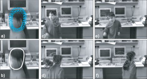
Figure 19.17 Tracking a contour through clutter. a) The representation of uncertainty about the contour consists of a set of weighted particles, each of which represents a hypothesis about the current position. In this frame, the different contours represent different hypotheses, and their weight indicates our relative belief that the system takes this state. b) The overall estimate of the current position can be illustrated by taking a weighted mean of the hypotheses. c-f) Four frames of sequence tracked by condensation algorithm showing the current estimate and the estimates from previous frames. Adapted from Blake and Isard (1998). ©1998 Springer.

Discussion

In this chapter we have discussed a family of models that allow us to estimate a set of continuous parameters throughout a time sequence by exploiting the temporal coherence of the estimates. In principle these methods can be applied to any model in this book that estimates a set of parameters from a single frame. These models have a close relationship with the chain-based models discussed in Chapter 11. The latter models used discrete parameters and generally estimated the state from the whole sequence rather than just the observed data up until the current time.

Notes

Applications of tracking: Tracking models are used for a variety of tasks in vision including tracking pedestrians (Rosales and Sclaroff 1999; Beymer and Konolige 1999), contours (Terzopolous and Szeliski 1992; Blake et al. 1993; 1995; Blake and Isard 1996; 1998), points (Broida and Chellappa 1986), 3D hand models (Stenger et al. 2001b), and 3D body models (Wang et al. 2008). They have also been used for activity recognition (Vaswani et al. 2003), estimating depth (Matthies et al. 1989), SLAM (Davison et al. 2007), and object recognition (Zhou et al. 2004). Reviews of tracking methods and applications can be found in Blake (2006) and Yilmaz et al. (2006). Approaches to tracking the human body are reviewed in Poppe (2007).

Tracking models: The Kalman filter was originally developed by Kalman (1960) and Kalman and Bucy (1961). The unscented Kalman filter was developed by Julier and Uhlmann (1997). The condensation algorithm is due to Blake and Isard (1996). For more information about the Kalman filter and its variants, consult Maybeck (1990), Gelb (1974), and Jazwinski (1970). Roweis and Ghahramani (1999) provide a unifying review of linear models, which provides information about how the Kalman filter relates to other methods. Arulampalam et al. (2002) provide a detailed review of the use of particle filters. A summary of tracking models and different approaches to inference within them can be found in Minka (2002).

There are a large number of variants on the standard Kalman filter. Many of these involve switching between different state space models or propagating mixtures (Shumway and Stoffer 1991; Ghahramani and Hinton 1996b; Murphy 1998; Chen and Liu 2000; Isard and Blake 1998). A notable recent extension has been to develop a nonlinear tracking algorithm based on the GPLVM (Wang et al. 2008).

One topic that has not been discussed in this chapter is how to learn the parameters of the tracking models. In practice, it is not uncommon to set these parameters by hand. However, information about learning in these temporal models can be found in Shumway and Stoffer (1982), Ghahramani and Hinton (1996a), Roweis and Ghahramani (2001), and Oh et al. (2005).

Simultaneous localization and mapping: Simultaneous localization and mapping has its roots in the robotics community who were concerned with the representation of spatial uncertainty by vehicles exploring an environment (Durrant-Whyte 1988; Smith and Cheeseman 1987), although the term SLAM was coined much later by Durrant-Whyte et al. (1996). Smith et al. (1990) had the important insight that the errors in mapped positions were correlated due to uncertainty in the camera position. The roots of vision-based SLAM are to be found in the pioneering work of Harris and Pike (1987), Ayache (1991), and Beardsley et al. (1995).

SLAM systems are usually based on either the extended Kalman filter (Guivant and Nebot 2001; Leonard and Feder 2000; Davison et al. 2007) or a Rao-Blackwellized particle filter (Montemerlo et al. 2002; Montemerlo et al. 2003; Sim et al. 2005). However, it currently the subject of some debate as to whether a tracking method of this type is necessary at all, or whether repeated bundle adjustments on tactically chosen subsets of 3D points will suffice (Strasdat et al. 2010).

Recent examples of efficient visual SLAM systems can be found in Nistér et al. (2004), Davison et al. (2007), Klein and Murray (2007), Mei et al. (2009), and Newcombe et al. (2011), and most of these include a bundle adjustment procedure into the algorithm. Current research issues in SLAM include how to efficiently match features in the image with features in the current model (Handa et al. 2010) and how to close loops (i.e., recognize that the robot has returned to a familiar place) in a map (Newman and Ho 2005). A review of SLAM techniques can be found in Durrant-Whyte and Bailey (2006) and Bailey and Durrant-Whyte (2006).

Problems

19.1 Prove the Chapman-Kolmogorov relation:

19.2 Derive the measurement incorporation step for the Kalman filter. In other words, show that

19.3 Consider a variation of the Kalman filter where the prior based on the previous time step is a mixture of K Gaussians

What will happen in the subsequent measurement incorporation step? What will happen in the next time update step?

19.4 Consider a model where there are two possible temporal update equations represented by state transition matrices Ψ₁ Ψ₂ and the system periodically switches from one regime to the other. Write a set of equations that describe this model and discuss a strategy for max-marginals inference.

19.5 In a Kalman filter model, discuss how you would compute the joint posterior distribution Pr(w_1…T|x_1…T) over all of the unknown world states. What form will this posterior distribution take? In the Kalman filter we choose to compute the max-marginals solution instead. Why is this?

19.6 Apply the sum-product algorithm (Section 11.4.3) to the Kalman filter model and show that the result is equivalent to applying the Kalman filter recursions.

19.7 Prove the Kalman smoother recursions:

where

Hint: It may help to examine the proof of the forward-backward algorithm for HMMs (Section 11.4.2).

19.8 Discuss how you would learn the parameters of the Kalman filter model given training sequences consisting of (i) both the known world state and the observed data and (ii) just the observed data alone.

19.9 In the unscented Kalman filter we represented a Gaussian with mean μ and covariance ∑ with a set of delta functions

with associated weights

Show that the mean and covariance of these points are indeed μ_t−1 and ∑_t−1 so that

19.10 The extended Kalman filter requires the Jacobian matrix describing how small changes in the data create small changes in the measurements. Compute the Jacobian matrix for the measurement model for the pedestrian-tracking application (Equation 19.50).

___________________________________

¹ In the original formulation of the Kalman filter, it was only assumed that the noise was white; however, if the distribution is normal, we can compute the exact marginal posterior distributions, so we will favor this assumption.