Computer Vision: Models, Learning, and Inference (2012)

Throughout this book, we have used iterative nonlinear optimization methods to find the maximum likelihood or MAP parameter estimates. We now provide more details about these methods. It is impossible to do full justice to this topic in the space available; many entire books have been written about nonlinear optimization. Our goal is merely to provide a brief introduction to the main ideas.

B.1 Problem statement

Continuous nonlinear optimization techniques aim to find the set of parameters that minimize a function f[•]. In other words, they try to compute

where f[•] is termed a cost function or objective function.

Although optimization techniques are usually described in terms of minimizing a function, most optimization problems in this book involve maximizing an objective function based on log probability. To turn a maximization problem into a minimization, we multiply the objective function by minus one. In other words, instead of maximizing the log probability, we minimize the negative log probability.

B.1.1 Convexity

The optimization techniques that we consider here are iterative: they start with an estimate θ^[0] and improve it by finding successive new estimates θ^[1], θ^[2],…,θ^[∞] each of which is better than the last until no more improvement can be made. The techniques are purely local in the sense that the decision about where to move next is based on only the properties of the function at the current position. Consequently, these techniques cannot guarantee the correct solution: they may find an estimate θ^[∞] from which no local change improves the cost. However, this does not mean there is not a better solution in some distant part of the function that has not yet been explored (Figure B.1). In optimization parlance, they can only find local minima. One way to mitigate this problem is to start the optimization from a number of different places and choose the final solution with the lowest cost.

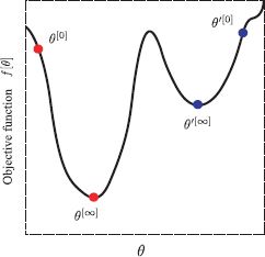
Figure B.1 Local minima. Optimization methods aim to find the minimum of the objective function f[θ] with respect to parameters θ. Roughly, they work by starting with an initial estimate θ^[0] and moving iteratively downhill until no more progress can be made (final position represented by θ^[∞]). Unfortunately, it is possible to terminate in a local minimum. For example, if we start at θ′^[0] and move downhill, we wind up in position θ′^[∞].

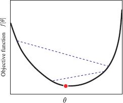
Figure B.2 Convex functions. If the function is convex, then the global minimum can be found. A function is convex if no chord (line between two points on the function) intersects the function. The figure shows two example chords (blue dashed lines). The convexity of a function can be established algebraically by considering the matrix of second derivatives. If this is positive definite for all values of θ, then the function is convex.

In the special case where the function is convex, there will only be a single minimum, and we are guaranteed to find it with sufficient iterations (Figure B.2). For a 1D function, it is possible to establish the convexity by looking at the second derivative of the function; if this is positive everywhere (i.e., the slope is continuously increasing), then the function is convex and the global minimum can be found. The equivalent test in higher dimensions is to examine the Hessian matrix (the matrix of second derivatives of the cost function with respect to the parameters). If this is positive definite everywhere (see Appendix C.2.6), then the function is convex and the global minimum will be found. Some of the cost functions in this book are convex, but this is unusual; most optimization problems found in vision do not have this convenient property.

B.1.2 Overview of approach

In general the parameters θ over which we search are multidimensional. For example, when θ has two dimensions, we can think of the function as a two-dimensional surface (Figure B.3). With this in mind, the principles behind the methods we will discuss are simple. We alternately

• Choose a search direction s based on the local properties of the function, and

• Search to find the minimum along the chosen direction. In other words, we seek the distance λ to move such that

and then set θ^[t+1] = θ^[t] + s. This is termed a line search.

We now consider each of these stages in turn.

B.2 Choosing a search direction

We will describe two general methods for choosing a search direction (steepest descent and Newton’s method) and one method which is specialized for least squares problems (the Gauss-Newton method). Both methods rely on computing derivatives of the function with respect to the parameters at the current position. To this end, we are relying on the function being smooth so that the derivatives are well behaved.

For most models, it is easy to find a closed form expression for the derivatives. If this is not the case, then an alternative is to approximate them using finite differences. For example, the first derivative of f[•] with respect to the j^thelement of θ can be approximated by

where a is a small number and e_j is the unit vector in the j^th direction. In principle as a tends to zero, this estimate becomes more accurate. However, in practice the calculation is limited by the floating point precision of the computer, so a must be chosen with care.

B.2.1 Steepest descent

An intuitive way to choose the search direction is to measure the gradient and select the direction which moves us downhill fastest. We could move in this direction until the function no longer decreases, then recompute the steepest direction and move again. In this way, we gradually move toward a local minimum of the function (Figure B.3a). The algorithm terminates when the gradient is zero and the second derivative is positive, indicating that we are at the minimum point, and any further local changes would not result in further improvement. This approach is termed steepest descent. More precisely, we choose

where the derivative ∂f/∂θ is the gradient vector that points uphill and λ is the distance moved downhill in the opposite direction −∂f/∂θ. The line search procedure (Section B.3) selects the value of λ.

Steepest descent sounds like a good idea but can be very inefficient in certain situations (Figure B.3b). For example, in a descending valley, it can oscillate ineffectually from one side to the other rather than proceeding straight down the center: the method approaches the bottom of the valley from one side, but overshoots because the valley itself is descending, so the minimum along the search direction is not exactly in the valley center (Figure B.3c). When we remeasure the gradient and perform a second line search, we overshoot in the other direction. This is not an unusual situation: it is guaranteed that the gradient at the new point will be perpendicular to the previous one, so the only way to avoid this oscillation is to hit the valley at exactly right angles.

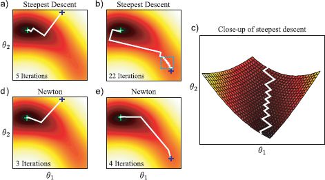
Figure B.3 Optimization on a two-dimensional function (color represents height of function). We wish to find the parameters that minimize the function (green cross). Given an initial starting point θ⁰ (blue cross), we choose a direction and then perform a local search to find the optimal point in that direction. a) One way to chose the direction is steepest descent: at each iteration, we head in the direction where the function changes the fastest. b) When we initialize from a different position, the steepest descent method takes many iterations to converge due to oscillatory behavior. c) Close-up of oscillatory region (see main text). d) Setting the direction using Newtons method results in faster convergence. e) Newtons method does not undergo oscillatory behavior when we initialize from the second position.

B.2.2 Newton’s method

Newton’s method is an improved approach that also exploits the second derivatives at the current point: it considers both the gradient of the function and how that gradient is changing.

To motivate the use of second derivatives, consider a one-dimensional function (Figure B.4). If the magnitude of the second derivative is low, then the gradient is changing slowly. Consequently, it will probably take a while before it completely flattens out and becomes a minimum, and so it is safe to move a long distance. Conversely, if the magnitude of the second derivative is high, then things are changing rapidly, and we should move only a small distance.

Now consider the same argument in two dimensions. Imagine we are at a point where the gradient is identical in both dimensions. For steepest descent, we would move equally in both dimensions. However, if the magnitude of the second derivative in the first direction is much greater than that in the second, we would nonetheless wish to move further in the second direction.

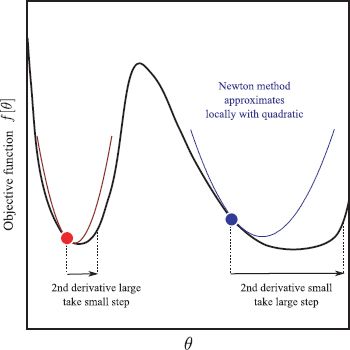
Figure B.4 Use of second derivatives. The gradient at the red and blue points is the same, but the magnitude of the second derivative is larger at the red point than the blue point: the gradient is changing faster at the red point than the blue point. The distance we move should be moderated by the second derivative: if the gradient is changing fast, then the minimum may be nearby and we should move a small distance. If it is changing slowly, then it is safe to move further. Newtons method takes into account the second derivative: it uses a Taylor expansion to create a quadratic approximation to the function and then moves toward the minimum.

To see how to exploit the second derivatives algebraically, consider a truncated Taylor expansion around the current estimate θ^[t]

where θ is a D × 1 variable, the first derivative vector is of size D × 1, and the Hessian matrix of second derivatives is D × D. To find the local extrema, we now take derivatives with respect to θ and set the result to zero

By rearranging this equation, we get an expression for the minimum ,

where the derivatives are still taken at θ^[t], but we have stopped writing this for clarity. In practice we would implement Newton’s method as a series of iterations

where the λ is the step size. This can be set to one, or we can find the optimal value using line search.

One interpretation of Newton’s method is that we have locally approximated the function as a quadratic. On each iteration, we move toward its extremum (or move exactly to it if we fix λ = 1). Note that we are assuming that we are close enough to the correct solution that the nearby extremum is a minimum and not a saddle point or maximum. In particular, if the Hessian is not positive definite, then a direction that is not downhill may be chosen. In this sense Newton’s method is not as robust as steepest descent.

Subject to this limitation, Newton’s method converges in fewer iterations than steepest descent (Figure B.3d-e). However, it requires more computation per iteration as we have to invert the D × D Hessian matrix at each step. Choosing this method usually implies that we can write the Hessian in closed form; approximating the Hessian from finite derivatives requires many function evaluations and so is potentially very costly.

B.2.3 Gauss-Newton method

Cost functions in computer vision often take the special form of a least squares problem

where g[•,•] is a function that transfers the variables {w_i} into the space of the variables {x_i}, and is parameterized by θ. In other words, we seek the values of θ that most closely map {w_i} to {x_i} in a least squares sense. This cost function is a special case of the more general form f[θ] = z^Tz, where

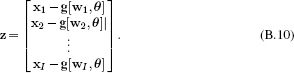
The Gauss-Newton method is an optimization technique that is used to solve least squares problems of the form

To minimize this objective function, we approximate the term z[θ] with a Taylor series expansion around the current estimate θ^[t] of the parameters:

where J is the Jacobian matrix. The entry j_mn at the m^th row and the n^th column of J contains the derivative of the m^th element of z with respect to the n^th parameter so that

Now we substitute the approximation for z[θ] into the original cost function f[θ] = z^Tz to yield

Finally, we take derivatives of this expression with respect to the parameters θ and equate to zero to get the relation

Rearranging, we get the update rule:

We can rewrite this by noting that

to give the final Gauss-Newton update

where the derivative is taken at θ^[t] and λ is the step size.

Comparing with the Newton update (Equation B.8), we see that we can consider this update as approximating the Hessian matrix as H ≈ J^TJ. It provides better results than gradient descent without ever computing second derivatives. Moreover, the term J^TJ is normally positive definite resulting in increased stability.

B.2.4 Other methods

There are numerous other methods for choosing the optimization direction. Many of these involve approximating the Hessian in some way with the goal of either ensuring that a downhill direction is always chosen or reducing the computational burden. For example, if computation of the Hessian is prohibitive, a practical approach is to approximate it with its own diagonal. This usually provides a better direction than steepest descent.

Quasi-Newton methods such as the Broyden Fletcher Goldfarb Shanno (BFGS) method approximate the Hessian with information gathered by analyzing successive gradient vectors. The Levenberg-Marquardt algorithm interpolates between the Gauss-Newton algorithm and steepest descent with the aim of producing a method that requires few iterations and is also robust. Damped Newton and trust-region methods also attempt to improve the robustness of Newton’s method. The nonlinear conjugate gradient algorithm is another valuable method when only first derivatives are available.

B.3 Line search

Having chosen a sensible direction using steepest descent, Newton’s method or some other approach, we must now decide how far to move: we need an efficient method to find the minimum of the function in the chosen direction. Line search methods start by determining the range over which to search for the minimum. This is usually guided by the magnitude of the second derivative along the line that provides information about the likely search range (see Figure B.4).

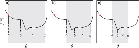
Figure B.5 Line search over region [a, d] using bracketing approach. Gray region indicates current search region. a) We define two points b, c that are interior to the search region and evaluate the function at these points. Here f[b] > f[c] so we eliminate the range [a, b]. b) We evaluate two points [b, c] interior to the new range and compare their values. This time we find that f[b] < f[c] so we eliminate the range [c, d]. c) We repeat this process until the minimum is closely bracketed.

There are many heuristics to find the minimum, but we will discuss only the direct search method (Figure B.5). Consider searching over the region [a, d]. We compute the function at two internal points b and c where a < b < c < d. If f[b] < f[c], we eliminate the range [c, d] and search over the new region [a, c] at the next iteration. Conversely, if f[b] > f[c], we eliminate the range [a, b] and search over a new region [b, d].

This method is applied iteratively until the minimum is closely bracketed. It is typically not worth exactly locating the minimum; the line search direction is rarely optimal and so the minimum of the line search is usually far from the overall minimum of the function. Once the remaining interval is sufficiently small, an estimate of the minimum position can be computed by making a parabolic fit to the three points that remain after eliminating one region or the other and selecting the position of the minimum of this parabola.

B.4 Reparameterization

Often in vision problems, we must find the best parameters θ subject to one or more constraints. Typical examples include optimizing variances σ² that must be positive, covariance matrices that must be positive definite, and matrices that represent geometric rotations which must be orthogonal. The general topic of constrained optimization is beyond the scope of this volume, but we briefly describe a trick that can be used to convert constrained optimization problems into unconstrained ones that can be solved using the techniques already described.

The idea of reparameterization is to represent the parameters θ in terms of a new set of parameters , which do not have any constraints on them, so that

where g[•] is a carefully chosen function.

Then we optimize with respect to the new unconstrained parameters . The objective function becomes f[g[]] and the derivatives are computed using the chain rule so that the first derivative would be

where θ_k is the k^th element of θ. This strategy is easier to understand with some concrete examples.

Parameters that must be positive

When we optimize a variance parameter θ = σ² we must ensure that the final answer is positive. To this end, we use the relation

and now optimize with respect to the new scalar parameter . Alternatively, we can use the square relation:

and again optimize with respect to the parameters .

Parameters that must lie between 0 and 1

To ensure that a scalar parameter θ lies between zero and one, we use the logistic sigmoid function:

and optimize with respect to the new scalar parameter .

Parameters that must be positive and sum to one

To ensure that the elements of a K × 1 multivariable parameter θ sum to one and are all positive we use the softmax function:

and optimize with respect to the new K × 1 variable .

3D rotation matrices

A 3 × 3 rotation matrix contains three independent quantities spread throughout its nine entries. A number of nonlinear constraints exist between the entries: the norm of each column and row must be one, each column is perpendicular to the other columns, each row is perpendicular to the other rows, and the determinant is one.

One way to enforce these constraints is to reparameterize the rotation matrix as a quaternion and optimize with respect to this new representation. A quaternion q is a 4D quantity q = [q₀, q₁, q₂, q₃]. Mathematically speaking, they are a four-dimensional extension of complex numbers, but the relevance for vision is that they can be used to represent 3D rotations. We use the relation:

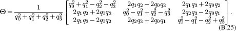
Although the quaternion contains four numbers, only the ratios of those numbers are important (giving 3 degrees of freedom): each element of Equation B.25 consists of squared terms, which are normalized by the squared amplitude constant, and so and constant that multiplies the elements of q is canceled out when we convert back to a rotation matrix.

Now we optimize with respect to the quaternion q. The derivatives with respect to the k^th element of q can be computed as

The quaternion optimization is stable as long as we do not approach the singularity at q = 0. One way to achieve this is to periodically renormalize the quaternion to length 1 during the optimization procedure.

Positive definite matrices

When we optimize over a K × K covariance matrix Θ = ∑, we must ensure that the result is positive definite. A simple way to do this is to use the relation:

where Φ is an arbitrary K × K matrix.