Computer Vision: Models, Learning, and Inference (2012)
Part VII
Appendices
Appendix C
Liner algebra
C.1 Vectors
A vector is a geometric entity in D dimensional space that has both a direction and a magnitude. It is represented by a D × 1 array of numbers. In this book, we write vectors as bold, small, Roman or Greek letters (e.g., a, ![]() ). The transpose aT of vector a is a 1 × D array of numbers where the order of the numbers is retained.
). The transpose aT of vector a is a 1 × D array of numbers where the order of the numbers is retained.
C.1.1 Dot product
The dot product or scalar product between two vectors a and b is defined as
![]()
where aT is the transpose of a (i.e., a converted to a row vector) and the returned value c is a scalar. Two vectors are said to be orthogonal if the dot product between them is zero.
C.1.2 Norm of a vector
The magnitude or norm of a vector is the square root of the sum of the square of the D elements so that
![]()
C.1.3 Cross product
The cross product or vector product is specialized to three dimensions. The operation c = a × b is equivalent to the matrix multiplication (Section C.2.1):
![]()
or for short
![]()
where A× is the 3 × 3 matrix from Equation C.3 that implements the cross product.
It is easily shown that the result c of the cross product is orthogonal to both a and b. In other words,
![]()
C.2 Matrices
Matrices are used extensively throughout the book and are written as bold, capital, Roman or Greek letters (e.g., A, Φ). We categorize matrices as landscape (more columns than rows), square (the same number of columns and rows), or portrait (more rows than columns). They are always indexed by row first and then column, so aij denotes the element of matrix A at the ith row and the jth column.
A diagonal matrix is a square matrix with zeros everywhere except on the diagonal (i.e., elements aii) where the elements may take any value. An important special case of a diagonal matrix is the identity matrix I. This has zeros everywhere except for the diagonal, where all the elements are ones.
C.2.1 Matrix multiplication
To take the matrix product C = AB, we compute the elements of C as
![]()
This can only be done when the number of columns in A equals the number of rows in B. Matrix multiplication is associative so that A(BC) = (AB)C = ABC. However, it is not commutative so that in general AB ≠ BA.
C.2.2 Transpose
The transpose of a matrix A is written as AT and is formed by reflecting it around the principal diagonal, so that the kth column becomes the kth row and vice versa. If we take the transpose of a matrix product AB, then we take the transpose of the original matrices but reverse the order so that
![]()
C.2.3 Inverse
A square matrix A may or may not have an inverse A−1 such that A−1 A = AA−1 = I. If a matrix does not have an inverse, it is called singular.
Diagonal matrices are particularly easy to invert: the inverse is also a diagonal matrix, with each diagonal value dii replaced by 1/dii. Hence, any diagonal matrix that has nonzero values on the diagonal is invertible. It follows that the inverse of the identity matrix is the identity matrix itself.
If we take the inverse of a matrix product AB, then we can equivalently take the inverse of each matrix individually, and reverse the order of multiplication
![]()
C.2.4 Determinant and trace
Every square matrix A has a scalar associated with it called the determinant and denoted by |A| or det[A]. It is (loosely) related to the scaling applied by the matrix. Matrices where the magnitude of the determinant is small tend to make vectors smaller upon multiplication. Matrices where the magnitude of the determinants is large tend to make them larger. If a matrix is singular, the determinant will be zero and there will be at least one direction in space that is mapped to the origin when the matrix is applied. For a diagonal matrix, the determinant is the product of the diagonal values. It follows that the determinant of the identity matrix is 1. Determinants of matrix expressions can be computed using the following rules:
![]()
![]()
![]()
The trace of a matrix is a second number associated with a square matrix A. It is the sum of the diagonal values (the matrix itself need not be diagonal). The traces of compound terms are bound by the following rules:
![]()
![]()
![]()
![]()
where in the last relation, the trace is invariant for cyclic permutations only, so that in general tr[ABC] ≠ tr[BAC].
C.2.5 Orthogonal and rotation matrices
An important class of square matrix is the orthogonal matrix. Orthogonal matrices have the following special properties:
1. Each column has norm one, and each row has norm one.
2. Each column is orthogonal to every other column, and each row is orthogonal to every other row.
The inverse of an orthogonal matrix Ω is its own transpose, so ΩTΩ = Ω−1Ω = I; orthogonal matrices are easy to invert! When this class of matrix premultiplies a vector, the effect is to rotate it around the origin and possibly reflect it.
Rotation matrices are a subclass of orthogonal matrices that have the additional property that the determinant is one. As the name suggests when this class of matrix premultiplies a vector, the effect is to rotate it around the origin with no reflection.
C.2.6 Positive definite matrices
A D × D real symmetric matrix A positive definite if xT Ax > 0 for all nonzero vectors x. Every positive definite matrix is invertible and its inverse is also positive definite. The determinant and trace of a symmetric positive definite matrix are always positive. The covariance matrix ∑ of a normal distribution is always positive definite.
C.2.7 Null space of a matrix
The right null space of a matrix A consists of the set of vectors x for which
![]()
Similarly, the left null space of a matrix A consists of the set of vectors for which
![]()
A square matrix only has a nontrivial null space (i.e., not just x = 0) if the matrix is singular (non-invertible) and hence the determinant is zero.
C.3 Tensors
We will occasionally have need for D > 2 dimensional quantities that we shall refer to as D-dimensional tensors. For our purposes a matrix can be thought of as the special case of a two-dimensional tensor, and a vector as the special case of a 1D tensor.
The idea of taking matrix products generalizes to higher dimensions and is denoted using the special notion ×n where n is the dimension over which we take the product. For example, the lth element fl of the tensor product f = A ×2b×3 c is given by
![]()
where l, m and n index the 3D tensor A, and b and c are vectors.
C.4 Linear transformations
When we premultiply a vector by a matrix this is called a linear transformation. Figure C.1 shows the results of applying several different 2D linear transformations (randomly chosen 2 × 2 matrices) to the 2D vectors that represent the points of the unit square. We can deduce several things from this figure. First, the point (0,0) at the origin in always mapped back onto itself. Second, collinear points remain collinear. Third, parallel lines are always mapped to parallel lines. Viewed as a geometric transformation, premultiplication by a matrix can account for shearing, scaling, reflection and rotation around the origin.
A different perspective on linear transformations comes from applying different transformations to points on the unit circle (Figure C.2). In each case, the circle is transformed to an ellipse. The ellipse can be characterized by its major axis (most elongated axis) and its minor axis (most compact axis), which are perpendicular to one another. This tells us something interesting: in general, there is a special direction in space (position on the original circle) that gets stretched the most (or compressed the least) by the transformation. Likewise there is a second direction that gets stretched the least or compressed the most.
C.5 Singular value decomposition
The singular value decomposition (SVD) is a factorization of a M × N matrix A such that
![]()
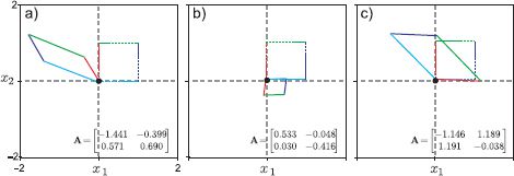
Figure C.1 Effect of applying three linear transformations to a unit square. Dashed square is before transformation. Solid square is after. The origin is always mapped to the origin. Colinear points remain colinear. Parallel lines remain parallel. The linear transformation encompasses shears, reflections, rotations, and scalings.
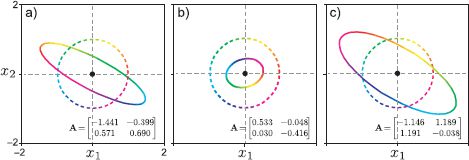
Figure C.2 Effect of applying three linear transformations to a circle. Dashed circle is before transformation. Solid ellipse is after. After the transformation, the circle is mapped to an ellipse. This demonstrates that there is one special direction that is expanded the most (becomes the major axis of the ellipse), and one special direction that is expanded the least (becomes the minor axis of the ellipse).
where U is a M × M orthogonal matrix, L is a M × N diagonal matrix, and V is a N × N orthogonal matrix. It is always possible to compute this factorization, although a description of how to do so is beyond the scope of this book.
The best way to get the flavor of the SVD is to consider some examples. First let us consider a square matrix:
Notice that by convention the nonnegative values on the principal diagonal of L decrease monotonically as we move from top-left to bottom-right. These are known as the singular values.
Now consider the singular value decomposition of a portrait matrix:
For this rectangular matrix, the orthogonal matrices U and V are different sizes and the diagonal matrix L is the same size as the original matrix. The singular values are still found on the diagonal, but the number is determined by the smallest dimension. In other words, if the original matrix was M × N then there will be a min[M, N] singular values.
To further understand the SVD, let us consider a third example:
![]()
Figure C.3 illustrates the cumulative effect of the transformations in the decomposition A3 = ULVT. The matrix VT rotates and reflects the original points. The matrix L scales the result differently along each dimension. In this case, it is stretched along the first dimension and shrunk along the second. Finally, the matrix U rotates the result.
Figure C.4 provides a second perspective on this process. Each pair of panels depicts what happens when we modify a different part of the SVD but keep the remaining parts the same. When we change V, the shape of the final ellipse is the same, but the mapping from original directions to points on the ellipse changes (observe the color change along the major axis). When we modify the first element of L, the length of the major axis changes. When we change the other nonzero element of L, the length of the minor axis changes. When we change the matrix U, the orientation of the ellipse changes.
C.5.1 Analyzing the singular values
We can learn a lot about a matrix by looking at the singular values. We saw in Section C.4, that as we decrease the smallest singular value the minor axis of the ellipse becomes progressively smaller. When it actually becomes zero, both sides of the unit circle collapse into one another (as do points from circles of all radii). Now there is a many-to-one mapping from the original points to the transformed ones and the matrix is no longer invertible. In general, a matrix is only invertible if all of the singular values are nonzero.
The number of nonzero singular values is called the rank of the matrix. The ratio of the smallest to the largest singular values is known as the condition number: it is roughly a measure of how ‘invertible’ the matrix is. As it becomes close to zero, our ability to invert the matrix decreases.
The singular values scale the different axes of the ellipse by different amounts (Figure C.3c). Hence, the area of a unit circle is changed by a factor that is equal to the product of the singular values. In fact, this scaling factor is the determinant (Section C.2.4). When the matrix is singular, at least one of the singular values is zero and hence the determinant is also zero. The right null space consists of all of the vectors that can be reached by taking a weighted sum of those columns of V whose corresponding singular values are zero. Similarly, the left null space consists of all of the vectors that can be reached by taking a weighted sum of those columns of U whose corresponding singular values are zero.
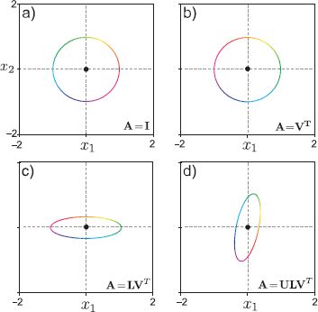
Figure C.3 Cumulative effect of SVD components for matrix A3. a) Original object. b) Applying matrix VT rotates and reflects the object around the origin. c) Subsequently applying L causes stretching/compression along the coordinate axes. d) Finally, applying matrix U rotates and reflects this distorted structure.
Orthogonal matrices only rotate and reflect points, and rotation matrices just rotate them. In either case, there is no change in area to the unit circle: all the singular values are one for these matrices and the determinant is also one.
C.5.2 Inverse of a matrix
We can also see what happens when we invert a square matrix in terms of the singular value decomposition. Using the rule (AB)−1 = B−1 A−1, we have
![]()
where we have used the fact that U and V are orthogonal matrices so U−1 = UT and V−1 = VT. The matrix L is diagonal so L−1 will also be diagonal with new nonzero entries that are the reciprocal of the original values. This also shows that the matrix is not invertible when any of the singular values are zero: we cannot take the reciprocal of 0.
Expressed in this way, the inverse has the opposite geometric effect to that of the original matrix: if we consider the effect on the transformed ellipse in Figure C.3d, it first rotates by UT so its major and minor axis are aligned with the coordinate axes (Figure C.3c). Then it scales these axes (using the elements of L−1), so that the ellipse becomes a circle (Figure C.3b). Finally, it rotates the result by V to get back to the original position (Figure C.3a).
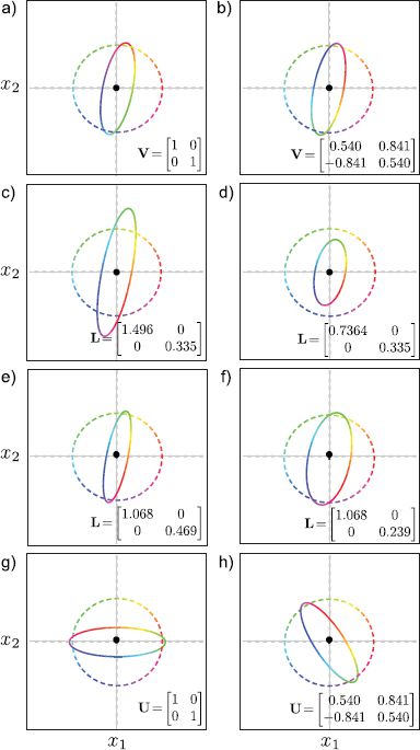
Figure C.4 Manipulating different parts of the SVD of A3. a-b) Changing matrix V does not affect the final ellipse, but changes which directions (colors) are mapped to the minor and major axes. c-d) Changing the first diagonal element of L changes the length of the major axis of the ellipse. e-f) Changing the second diagonal element of L changes the length of the minor axis. g-h) Changing U affects the final orientation of the ellipse.
C.6 Matrix calculus
We are often called upon to take derivatives of compound matrix expressions. The derivative of a function f[a] that takes a vector as its argument and returns a scalar is a vector b with elements
![]()
The derivative of a function f[A] that returns a scalar, with respect to an M × N matrix A will be a M × N matrix B with elements
![]()
The derivative of a function f[a] that returns a vector with respect to vector a is a matrix B with elements
![]()
where fi is the ith element of the vector returned by the function f[a].
We now provide several commonly used results for reference.
1. Derivative of linear function:
![]()
![]()
![]()
![]()
2. Derivative of quadratic function:
![]()
![]()
![]()
![]()
![]()
3. Derivative of determinant:
![]()
which leads to the relation
![]()
4. Derivative of log determinant:
![]()
5. Derivative of inverse:
![]()
6. Derivative of trace:
![]()
More information about matrix calculus can be found in Peterson et al. (2006).
C.7 Common problems
In this section, we discuss several standard linear algebra problems that are found repeatedly in computer vision.
C.7.1 Least squares problems
Many inference and learning tasks in computer vision result in least squares problems. The most frequent context is when we use maximum likelihood methods with the normal distribution. The least squares problem may be formulated in a number of ways. We may be asked to find the vector x that solves the system
![]()
in a least squares sense. Alternatively, we may be given i of smaller sets of equations of the form
![]()
and again asked to solve for x. In this latter case, we form the compound matrix A = [AT1, AT2…ATI]T and compound vector b = [bT1, bT2…bTI]T, and the problem is the same as in Equation C.41.
We may equivalently see the same problem in an explicit least squares form,
![]()
Finally, we may be presented the problem as a sum of smaller terms
![]()
in which case we form compound matrices A and b, which changes the problem back to that in Equation C.43.
To make progress, we multiply out the terms in Equation C.43
where we have combined two terms in the last line by noting that they are both the same: they are transposes of one another, but they are also scalars, so they equal their own transpose. Now we take the derivative with respect to xand equate the result to zero to give
![]()
which we can rearrange to give the standard least squares result
![]()
This result can only be computed if there are at least as many rows in A as there are unknown values in x (i.e., if the matrix A is square or portrait). Otherwise, the matrix AT A will be singular. For implementations in Matlab, it is better to make use of the backslash operator ‘\’ rather than explicitly implement Equation C.47.
C.7.2 Principal direction/minimum direction
We define the principal and minimal directions as
respectively. This problem has exactly the geometric form of Figure C.2. The constraint that |b| = 1 means that b has to lie on the circle (or sphere or hypersphere in higher dimensions). In the principal direction problem, we are hence seeking the direction that is mapped to the major axis of the resulting ellipse/ellipsoid. In the minimum direction problem, we seek the direction that is mapped to the minor axis of the ellipsoid.
We saw in Figure C.4 that it is the matrix V from the singular value decomposition of A that controls which direction is mapped to the different axes of the ellipsoid. To solve the principal direction problem, we hence compute the SVD, A = ULVT and set b to be the first column of V. To solve the minimum direction problem, we set b to be the last column of V.
C.7.3 Orthogonal Procrustes problem
The orthogonal Procrustes problem is to find the closest linear mapping Ω between one set of vectors A and another B such that Ω is an orthogonal matrix. In layman’s terms, we seek the best Euclidean rotation (possibly including mirroring) that maps points A to points B.
![]()
where |•|F denotes the Frobenius norm of a matrix - the sum of the square of all of the elements. To make progress, we recall that the trace of a matrix is the sum of its diagonal entries and so |X|F = tr[XT X], which gives the new criterion
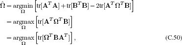
where we have used relation C.15 between the last two lines. We now compute the SVD BAT = ULVT to get the criterion
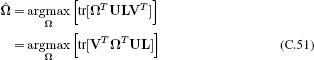
and notice that
![]()
where we defined Z = VT ΩT U and used the fact that the L is a diagonal matrix, so each entry scales the diagonal of Z on multiplication.
We note that the matrix Z is orthogonal (it is the product of three orthogonal matrices). Hence, every value on the diagonal of the orthogonal matrix Z must be less than or equal to one (the norms of each column are exactly one), and so we maximize the criterion in Equation C.25 by choosing Z = I when the diagonal values are equal to one. To achieve this, we set ΩT = VUT so that the overall solution is
![]()
A special case of this problem is to find the closest orthogonal matrix Ω to a given square matrix B in a least squares sense. In other words, we seek to optimize
![]()
This is clearly equivalent to optimizing the criterion in Equation C.49 but with A = I. It follows that the solution can be found by computing the singular value decomposition B = ULVT and setting Ω = UVT.
C.8 Tricks for inverting large matrices
Inversion of a D × D matrix has a complexity of ![]() (D3). In practice, this means it is difficult to invert matrices whose dimension is larger than a few thousand. Fortunately, matrices are often highly structured, and we can exploit that structure using a number of tricks to speed up the process.
(D3). In practice, this means it is difficult to invert matrices whose dimension is larger than a few thousand. Fortunately, matrices are often highly structured, and we can exploit that structure using a number of tricks to speed up the process.
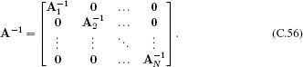
C.8.1 Diagonal and block-diagonal matrices
Diagonal matrices can be inverted by forming a new diagonal matrix, where the values on the diagonal are reciprocal of the original values. Block diagonal matrices are matrices of the form
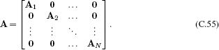
The inverse of a block-diagonal matrix can be computed by taking the inverse of each block separately so that
C.8.2 Inversion relation #1: Schur complement identity
The inverse of a matrix with sub-blocks A, B, C, and D in the top-left, top-right, bottom-left, and bottom-right positions, respectively, can easily be shown to be
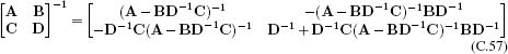
by multiplying the original matrix with the right-hand side and showing that the result is the identity matrix.
This result is extremely useful when the matrix D is diagonal or block-diagonal (Figure C.5). In this circumstance, D−1 is fast to compute, and the remaining inverse quantity (A − BD−1C)−1 is much smaller and easier to invert than the original matrix. The quantity A − BD−1C is known as the Schur complement.
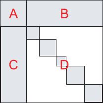
Figure C.5 Inversion relation #1. Gray regions indicate parts of matrix with nonzero values, white regions represent zeros. This relation is suited to the case where the matrix can be divided into four submatrices A, B, C, D, and the bottom right block is easy to invert (e.g., diagonal, block diagonal or structured in another way that means that inversion is efficient). After applying this relation, the remaining inverse is the size of submatrix A.
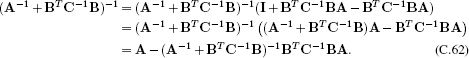
C.8.3 Inversion relation #2
Consider the d × d matrix A, the k × k matrix C, and the k × d matrix B where A and C are symmetric, positive definite matrices. The following equality holds:
![]()
Proof:
![]()
Taking the inverse of both sides we get
![]()
as required
This relation is very useful when B is a landscape matrix with many more columns C than rows R. On the left-hand side, the term we must invert is of size C × C, which might be very costly. However, on the right-hand side, the inversion is only of size R × R, which might be considerably more cost efficient.
C.8.4 Inversion relation #3: Sherman-Morrison-Woodbury
Consider the d × d matrix A, the k × k matrix C and the k × d matrix B where A and C are symmetric, positive definite matrices. The following equality holds:
![]()
This is sometimes known as the matrix inversion lemma.
Proof:
Now, applying inversion relation #2 to the term in brackets:
![]()
as required.
C.8.5 Matrix determinant lemma
The matrices that we need to invert are often the covariances in the normal distribution. When this is the case, we sometimes also need to compute the determinant of the same matrix. Fortunately, there is a direct analogy of the matrix inversion lemma for determinants.
Consider the d × d matrix A, the k × k matrix C and the k × d matrix B where A and C are symmetric, positive definite covariance matrices. The following equality holds:
![]()
All materials on the site are licensed Creative Commons Attribution-Sharealike 3.0 Unported CC BY-SA 3.0 & GNU Free Documentation License (GFDL)
If you are the copyright holder of any material contained on our site and intend to remove it, please contact our site administrator for approval.
© 2016-2026 All site design rights belong to S.Y.A.