Computer Vision: Models, Learning, and Inference (2012)

Part II

Machine learning for machine vision

Chapter 9

Classification models

This chapter concerns discriminative models for classification. The goal is to directly model the posterior probability distribution Pr(w|x) over a discrete world state w ∈{1,… K} given the continuous observed data vector x. Models for classification are very closely related to those for regression and the reader should be familiar with the contents of Chapter 8 before proceeding.

To motivate the models in this chapter, we will consider gender classification: here we observe a 60 × 60 RGB image containing a face (Figure 9.1) and concatenate the RGB values to form the 10800 × 1 vector x. Our goal is to take the vector x and return the probability distribution Pr(w|x)over a label w ∈ {0, 1} indicating whether the face is male (w = 0) or female (w = 1).

Gender classification is a binary classification task as there are only two possible values of the world state. Throughout most of this chapter, we will restrict our discussion to binary classification. We discuss how to extend these models to cope with an arbitrary number of classes in Section 9.9.

9.1 Logistic regression

We will start by considering logistic regression, which despite its name is a model that can be applied to classification. Logistic regression (Figure 9.2) is a discriminative model; we select a probability distribution over the world state w ∈ {0, 1} and make its parameters contingent on the observed data x. Since the world state is binary, we will describe it with a Bernoulli distribution, and we will make the single Bernoulli parameter λ (indicating the probability that the world state takes the value w = 1) a function of the measurements x.

In contrast to the regression model, we cannot simply make the parameter λ a linear function ₀ + ^Tx of the measurements; a linear function can return any value, but the parameter λ must lie between 0 and 1. Consequently, we first compute the linear function and then pass this through the logistic sigmoid function sig [•] that maps the range [−∞, ∞] to [0, 1]. The final model is hence

where a is termed the activation and is given by the linear function

Figure 9.1 Gender classification. Consider a 60×60 pixel image of a face. We concatenate the RGB values to make a 10800 × 1 data vector x. The goal of gender classification is to use the data x to infer a label w ∈{0, 1} indicating whether the window contains a) a male or b) a female face. This is challenging because the differences are subtle and there is image variation due to changes in pose, lighting, and expression. Note that real systems would preprocess the image before classification by registering the faces more closely and compensating in some way for lighting variation (see Chapter 13).

The logistic sigmoid function sig[•] is given by

As the activation a tends to ∞ this function tends to one. As a tends to −∞ it tends to zero. When a is zero, the logistic sigmoid function returns a value of one half.

For 1D data x, the overall effect of this transformation is to describe a sigmoid curve relating x to λ (Figures 9.2c and 9.3a). The horizontal position of the sigmoid is determined by the place that the linear function a crosses zero (i.e., the x-intercept) and the steepness of the sigmoid depends on the gradient ₁.

In more than one dimension, the relationship between x and λ is more complex (Figure 9.3b). The predicted parameter λ has a sigmoid profile in the direction of the gradient vector but is constant in all perpendicular directions. This induces a linear decision boundary. This is the set of positions in data space {x : Pr(w = 1|x) = 0.5} where the posterior probability is 0.5; the decision boundary separates the region where the world state w is more likely to be 0 from the region where it is more likely to be 1. For logistic regression, the decision boundary takes the form of a hyperplane with the normal vector in the direction of .

As for regression, we can simplify the notation by attaching the y-intercept ₀ to the start of the parameter vector so that ← [₀ ^T]^T and attaching 1 to the start of the data vector x so that x ← [1 x^T]^T. After these changes, the activation is now a = ^Tx, and the final model becomes

Notice that this is very similar to the linear regression model (Section 8.1) except for the introduction of the nonlinear logistic sigmoid function sig[•] (explaining the unfortunate name “logistic regression”). However, this small change has serious implications: maximum likelihood learning of the parameters is considerably harder than for linear regression and to adopt the Bayesian approach we will be forced to make approximations.

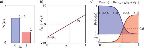
Figure 9.2 Logistic regression. a) We represent the world state w as a Bernoulli distribution and make the Bernoulli parameter λ a function of the observations x. b) We compute the activation a as a linear sum a = ₀ + ₁x of the observations. c) The Bernoulli parameter λ is formed by passing the activation through a logistic sigmoid function sig[•] to constrain the value to lie between 0 and 1, giving the characteristic sigmoid shape. In learning, we fit parameters θ = {₀, ₁} using training pairs {x_i, w_i}. In inference, we take a new datum x* and evaluate the posterior Pr(w*|x*) over the state.

9.1.1 Learning: maximum likelihood

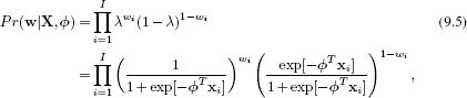
In maximum likelihood learning, we consider fitting the parameters using I paired examples of training data {x_i, w_i}^I_i=1 (Figure 9.3). Assuming independence of the training pairs we have

where X = [x₁,x₂,…,x_I] is a matrix containing the measurements and w = [w₁,w₂,…,w_I]^T is a vector containing all of the binary world states. The maximum likelihood method finds parameters , which maximize this expression.

As usual, however, it is simpler to maximize the logarithm L of this expression. Since the logarithm is a monotonic transformation, it does not change the position of the maximum with respect to . Applying the logarithm replaces the product with a sum so that

The derivative of the log likelihood L with respect to the parameters is

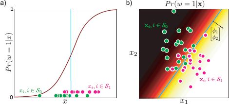
Figure 9.3 Logistic regression model fitted to two different data sets. a) One dimensional data. Green points denote set of examples S₀ where w = 0. Pink points denote S₁ where w = 1. Note that in this (and all future figures in this chapter), we have only plotted the probability Pr(w = 1|x) (compare to Figure 9.2c). The probability Pr(w = 0|x) can be computed as 1 – Pr(w = 1|x). b) Two-dimensional data. Here, the model has a sigmoid profile in the direction of the gradient and Pr(w = 1|x) is constant in the orthogonal directions. The decision boundary (cyan line) is linear.

Unfortunately, when we equate this expression to zero, there is no way to re-arrange to get a closed form solution for the parameters . Instead, we must rely on a nonlinear optimization technique to find the maximum of this objective function. Optimization techniques are discussed in detail in Appendix B. In brief, we start with an initial estimate of the solution and iteratively improve it until no more progress can be made.

Here, we will apply the Newton method, in which we base the update of the parameters on the first and second derivatives of the function at the current position so that

where ^[t] denotes the estimate of the parameters at iteration t and α determines how much we change this estimate and is usually chosen by an explicit search at each iteration.

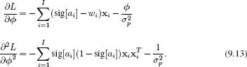
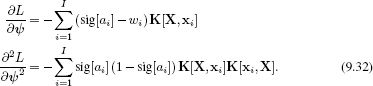
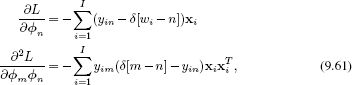
For the logistic regression model, the D×1 vector of first derivatives and the D×D matrix of second derivatives are given by

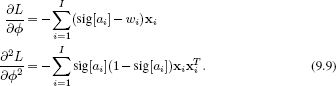
These are known as the gradient vector and the Hessian matrix, respectively.¹

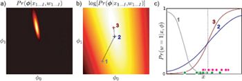
Figure 9.4 Parameter estimation for logistic regression with 1D data. a) In maximum likelihood learning, we seek the maximum of Pr(w|X, ) with respect to . b) In practice, we instead maximize log likelihood: notice that the peak is in the same place. Crosses show results of two iterations of optimization using Newton’s method. c) The logistic sigmoid functions associated with the parameters at each optimization step. As the log likelihood increases, the model fits the data more closely: the green points represent data where w = 0 and the purple points represent data where w = 1 and so we expect the best-fitting model to increase from left to right just like curve 3.

The expression for the gradient vector has an intuitive explanation. The contribution of each datapoint depends on the difference between the actual class w_i and the predicted probability λ = sig[a_i] of being in class 1; points that are classified incorrectly contribute more to this expression and hence have more influence on the parameter values. Figure 9.4 shows maximum likelihood learning of the parameters for 1D data using a series of Newton steps.

For general functions, the Newton method only finds local maxima. At the end of the procedure, we cannot be certain that there is not a taller peak in the likelihood function elsewhere. However, the log likelihood for logistic regression has a special property. It is a concave function of the parameters . For concave functions there are never multiple maxima and gradient-based approaches are guaranteed to find the global maximum. It is possible to establish whether a function is concave or not by examining the Hessian matrix. If this is negative definite for all , then the function is concave. This is the case for logistic regression as the Hessian (Equation 9.9) consists of a negative weighted sum of outer products.²

9.1.2 Problems with the logistic regression model

The logistic regression model works well for simple data sets, but for more complex visual data it will not generally suffice. It is limited in the following ways.

1. It is overconfident as it was learned using maximum likelihood.

2. It can only describe linear decision boundaries.

3. It is inefficient and prone to overfitting in high dimensions.

In the remaining part of this chapter, we will extend this model to cope with these problems (Figure 9.5).

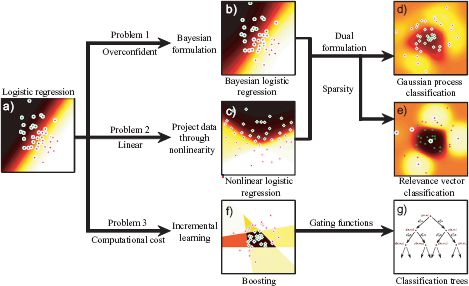
Figure 9.5 Family of classification models. a) In the remaining part of the chapter, we will address several of the limitations of logistic regression for binary classification. b) The logistic regression model with maximum likelihood learning is overconfident, and hence we develop a Bayesian version. c) It is unrealistic to always assume a linear relationship between the data and the world, and to this end we introduce a nonlinear version. d) Combining the Bayesian and nonlinear versions of regression leads to Gaussian process classification. e) The logistic regression model also has many parameters and may require considerable resources to learn when the data dimension is high, and so we develop relevance vector classification that encourages sparsity. f) We can also build a sparse model by incrementally adding parameters in a boosting scheme. g) Finally, we consider a very fast classification model based on a tree structure.

9.2 Bayesian logistic regression

In the Bayesian approach, we learn a distribution Pr(|X, w) over the possible parameter values that are compatible with the training data. In inference, we observe a new data example x* and use this distribution to weight the predictions for the world state w* given by each possible estimate of . In linear regression (Section 8.2), there were closed form expressions for both of these steps. However, the nonlinear function sig[•]in logistic regression means that this is no longer the case. To get around this, we will approximate both steps so that we retain neat closed form expressions and the algorithm is tractable.

9.2.1 Learning

We start by defining a prior over the parameters . Unfortunately, there is no conjugate prior for the likelihood in the logistic regression model (Equation 9.1); this is why there won’t be closed form expressions for the likelihood and predictive distribution. With nothing else to guide us, a reasonable choice for the prior over the continuous parameters is a multivariate normal distribution with zero mean and a large spherical covariance so that

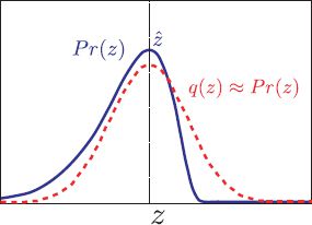
Figure 9.6 Laplace approximation. A probability density (blue curve) is approximated by a normal distribution (red curve). The mean of the normal (and hence the peak) is chosen to coincide with the peak of the original pdf. The variance of the normal is chosen so that its second derivatives at the mean match the second derivatives of the original pdf at the peak.

To compute the posterior probability distribution Pr(|X, w) over the parameters given the training data pairs {x_i, w_i}, we apply Bayes’ rule,

where the likelihood and prior are given by Equations 9.5 and 9.10, respectively. Since we are not using a conjugate prior, there is no simple closed form expression for this posterior and so we are forced to make an approximation of some kind.

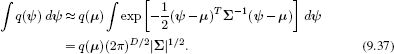
One possibility is to use the Laplace approximation (Figure 9.6) which is a general method for approximating complex probability distributions. The goal is to approximate the posterior distribution by a multivariate normal. We select the parameters of this normal so that (i) the mean is at the peak of the posterior distribution (i.e., at the MAP) and (ii) the covariance is such that the second derivatives at the peak match the second derivatives of the true posterior distribution at its peak.

Hence, to make the Laplace approximation, we first find the MAP estimate of the parameters and to this end we use a nonlinear optimization technique such as Newton’s method to maximize the criterion,

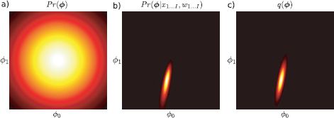
Figure 9.7 Laplace approximation for logistic regression. a) The prior Pr() over the parameters is a normal distribution with mean zero and a large spherical covariance. b) The posterior distribution Pr(|X,w) represents the refined state of our knowledge after observing the data. Unfortunately, this posterior cannot be expressed in closed form. c) We approximate the true posterior with a normal distribution q() = Norm [μ,Σ] whose mean is at the peak of the posterior and whose covariance is chosen so that the second derivatives at the peak of the true posterior match the second derivatives at the peak of the normal. This is termed the Laplace approximation.

Newton’s method needs the derivatives of the log posterior which are

We then approximate the posterior by a multivariate normal so that

where the mean μ is set to the MAP, estimate and the covariance Σ is chosen so that the second derivatives of the normal match those of the log posterior at the MAP estimate (Figure 9.7) so that

9.2.2 Inference

In inference we aim to compute a posterior distribution Pr(w*|x*, X, w) over the world state w* given new observed data x*. To this end, we compute an infinite weighted sum (i.e., an integral) of the predictions Pr(w*|x*,) given by each possible value of the parameters ,

where the weights q() are given by the approximated posterior distribution over the parameters from the learning stage. Unfortunately, this integral cannot be computed in closed form either, and so we must make a further approximation.

We first note that the prediction Pr(w*|x*,) depends only on a linear projection a = ^T x* of the parameters (see Equation 9.4). Hence we could reexpress the prediction as

The probability distribution Pr(a) can be computed using the transformation property of the normal distribution (Section 5.3) and is given by

where we have denoted the mean and variance of the activation by μ_a and σ_a², respectively. The one-dimensional integration in Equation 9.17 can now be computed using numerical integration over a, or we can approximate the result with a similar function such as

It is not obvious by inspection that this function should approximate the integral well; however, Figure 9.8 demonstrates that the approximation is quite accurate.

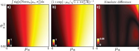
Figure 9.8 Approximation of activation integral (Equation 9.19). a) Actual result of integral as a function of μ_a and σ²_a. b) The (nonobvious) approximation from Equation 9.19. c) The absolute difference between the actual result and the approximation is very small over a range of reasonable values.

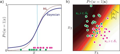
Figure 9.9 Bayesian logistic regression predictions. a) The Bayesian prediction for the class w is more moderate than the maximum likelihood prediction. b) In 2D the decision boundary in the Bayesian case (blue line) is still linear but iso-probability contours at levels other than 0.5 are curved (compare to maximum likelihood case in Figure 9.3b). Here too, the Bayesian solution makes more moderate predictions than the maximum likelihood model.

Figure 9.9 compares the classification predictions Pr(w*|x*) for the maximum likelihood and Bayesian approaches for logistic regression. The Bayesian approach makes more moderate predictions for the final class. This is particularly the case in regions of data space that are far from the mean.

9.3 Nonlinear logistic regression

The logistic regression model described previously can only create linear decision boundaries between classes. To create nonlinear decision boundaries, we adopt the same approach as we did for regression (Section 8.3): we compute a nonlinear transformation z = f [x] of the observed data and then build the logistic regression model substituting the original data x for the transformed data z, so that

The logic of this approach is that arbitrary nonlinear activations can be built as a linear sum of nonlinear basis functions. Typical nonlinear transformations include

• Heaviside step functions of projections: z_k = heaviside[α^T_kx],

• Arc tangent functions of projections: z_k = arctan[α^T_kx], and

• Radial basis functions:

where z_k denotes the k^th element of the transformed vector z and the function heaviside[•] returns zero if its argument is less than zero and one otherwise. In the first two cases we have attached a 1 to the start of the observed data xwhere we use projections α^Tx to avoid having a separate offset parameter. Figures 9.10 and 9.11 show examples of nonlinear classification using arc tangent functions for one and two-dimensional data, respectively.

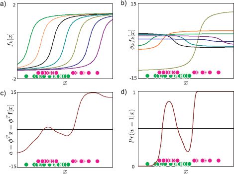
Figure 9.10 Nonlinear classification in 1D using arc tangent transformation. We consider a complex 1D data set (bottom of all panels) where the posterior Pr(w = 1|x) cannot easily be described by a single sigmoid. Green circles represent data x_i where w_i = 0. Pink circles represent data x_i where w_i = 1. a) The seven dimensional transformed data vectors z₁…z_I are computed by evaluating each data example against seven predefined arc tangent functions z_ik = f_k[x_i] = arctan[α_0k + α_1kx_i]. b) When we learn the parameters , we are learning weights for these nonlinear arc tangent functions. The functions are shown after applying the maximum likelihood weights . c) The final activation a = ^Tz is a weighted sum of the nonlinear functions. d) The probability Pr(w = 1|x) is computed by passing the activation a through the logistic sigmoid function.

Note that the basis functions also have parameters. For example, in the arc tangent example, there are the projection directions {α_k}^K_k=1, each of which contains an offset and a set of gradients. These can also be optimized during the fitting procedure together with the weights . We form a new vector of unknowns θ = [^T,α^T₁,α^T₂,…α^T_K]^T and optimize the model with respect to all of these unknowns together. The gradient vector and the Hessian matrix depend on the chosen transformation f[•] but can be computed using the expressions

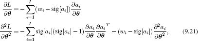
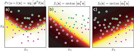
Figure 9.11 Nonlinear classification in 2D using arc tangent transform. a) These data have been successfully classified with nonlinear logistic regression. Note the nonlinear decision boundary (cyan line). To compute the posterior Pr(w = 1|x), we transform the data to a new two-dimensional space z = f[x] where the elements of z are computed by evaluating x against the 1D arc tangent functions in b) and c). The arc tangent activations are weighted (the first by a negative number) and summed and the result is put through the logistic sigmoid to compute Pr(w = 1|x).

where a_i = ^Tf[x_i]. These relations were established using the chain rules for derivatives. Unfortunately, this joint optimization problem is generally not convex and will be prone to terminating in local maxima. In the Bayesian case, it would be typical to marginalize over the parameters but maximize over the function parameters.

9.4 Dual logistic regression

There is a potential problem with the logistic regression models as described earlier: in the original linear model, there is one element of the gradient vector corresponding to each dimension of the observed data x, and in the nonlinear extension there is one element corresponding to each transformed data dimension z. If the relevant data x (or z) is very high-dimensional, then the model will have a large number of parameters: this will render the Newton update slow or even intractable. To solve this problem, we switch to the dual representation. For simplicity, we will develop this model using the original data x, but all of the ideas transfer directly to the nonlinear case where we use transformed data z.

In the dual parameterization, we express the gradient parameters as a weighted sum of the observed data (see Figure 8.12) so that

where ψ is an I × 1 variable in which each element weights one of the data examples. If the number of data points is less than the dimensionality D of the data x, then the number of parameters has been reduced.

The price that we pay for this reduction is that we can now only choose gradient vectors that are in the space spanned by the data examples. However, the gradient vector represents the direction in which the final probability Pr(w = 1|x) changes fastest, and this should not point in a direction in which there was no variation in the training data anyway, so this is not a limitation.

Substituting Equation 9.22 into the original logistic regression model leads to the dual logistic regression model,

The resulting learning and inference algorithms are very similar to those for the original logistic regression model, and so we cover them only in brief:

• In the maximum likelihood method, we learn the parameters ψ by nonlinear optimization of the log likelihood L = log[Pr(w|X,ψ)] using the Newton method. This optimization requires the derivatives of the log likelihood, which are

• In the Bayesian approach, we use a normal prior over the parameters ψ,

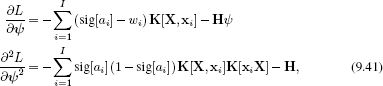
The posterior distribution Pr(ψ|X, w) over the new parameters is found using Bayes’ rule, and once more this cannot be written in closed form, so we apply the Laplace approximation. We find the MAP solution using nonlinear optimization, which requires the derivatives of the log posterior L = log[Pr(ψ|X, w)]:

The posterior is now approximated by a multivariate normal so that

where

In inference, we compute the distribution over the activation

and then approximate the predictive distribution using Equation 9.19.

Dual logistic regression gives identical results to the original logistic regression algorithm for the maximum likelihood case and very similar results in the Bayesian situation (where the difference results from the slightly different priors). However, the dual classification model is much faster to fit in high dimensions as the parameters are fewer.

9.5 Kernel logistic regression

We motivated the dual model by the reduction in the number of parameters ψ in the model when the data lies in a high-dimensional space. However, now that we have developed the model, a further advantage is easy to identify: both learning and inference in the dual model rely only on inner products x^T_i x_j of that data. Equivalently, the nonlinear version of this algorithm depends only on inner products z^T_i z_j of the transformed data vectors. This means that the algorithm is suitable for kernelization (see Section 8.4).

The idea of kernelization is to define a kernel function k[•,•], which computes the quantity

where z_i = f[x_i] and z_j = f[x_j] are the nonlinear transformations of the two data vectors. Replacing the inner products with the kernel function means that we do not have to explicitly calculate the transformed vectors z, and hence they may be of very high, or even infinite dimensions. See Section 8.4 for a more detailed description of kernel functions.

The kernel logistic regression model (compare to Equation 9.23) is hence

where the notation K[X, x]_i represents a column vector of dot products where element k is given by k[x_k, x_i].

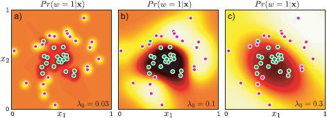
Figure 9.12 Kernel logistic regression using RBF kernel and maximum likelihood learning. a) With a small length scale λ, the model does not interpolate much from the data examples. b) With a reasonable length scale, the classifier does a good job of modeling the posterior Pr(w = 1|x). c) With a large length scale, the estimated posterior is very smooth and the model interpolates confident decisions into regions such as the top-left where there is no data.

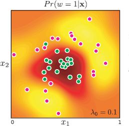
Figure 9.13 Kernel logistic regression with RBF kernel in a Bayesian setting: we now take account of our uncertainty in the dual parameters ψ by approximating their posterior distribution using Laplace’s method and marginalizing them out of the model. This produces a very similar result to the maximum likelihood case with the same length scale (Figure 9.12b). However, as is typical with Bayesian implementations, the confidence is (appropriately) somewhat lower.

For maximum likelihood learning, we simply optimize the log posterior probability L with respect to the parameters, which requires the derivatives:

The Bayesian formulation of kernel logistic regression, which is sometimes known as Gaussian process classification, proceeds along similar lines; we follow the dual formulation, replacing each the dot products between data examples with the kernel function.

A very common example of a kernel function is the radial basis kernel in which the nonlinear transformation and inner product operations are replaced by

This is equivalent to computing transformed vectors z_i and z_j of infinite length, where each entry evaluates the data x against a radial basis function at a different position, and then computing the inner product z^T_i z_j. Examples of the kernel logistic regression with a radial basis kernel are shown in Figures 9.12 and 9.13.

9.6 Relevance vector classification

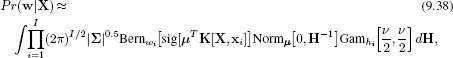
The Bayesian version of the kernel logistic regression model is powerful, but computationally expensive as it requires us to compute dot products between the new data example and the all of the training examples (in the kernel function in Equation 9.31). It would be more efficient if the model depended only sparsely on the training data. To achieve this, we impose a penalty for every nonzero weighted training example. As in the relevance regression model (Section 8.8), we replace the normal prior over the dual parameters ψ (Equation 9.25) with a product of one-dimensional t-distributions so that

Applying the Bayesian approach to this model with respect to the parameters Ψ is known as relevance vector classification.

Following the argument of Section 8.6, we rewrite each student t-distribution as a marginalization of a joint distribution Pr(ψ_i,h_i)

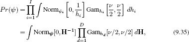
where the matrix H contains the hidden variables {h_i}^I_i=1 on its diagonal and zeros elsewhere. Now we can write the model likelihood as

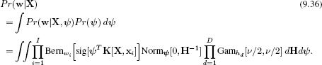
Now we make two approximations. First, we use the Laplace approximation to describe the first two terms in this integral as a normal distribution with mean μ and covariance ∑ centered at the MAP parameters, and use the following result for the integral over ψ:

This yields the expression

where the matrix H contains the hidden variables {h_i}^I_i=1 on the diagonal.

In the second approximation, we maximize over the hidden variables, rather than integrate over them. This yields the expression:

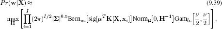
To learn the model, we now alternate between updating the mean and variance μ and ∑ of the posterior distribution and updating the hidden variables {h_i}. To update the mean and variance parameters, we find the solution that maximizes

using the derivatives

and then set

To update the hidden variables h_i we use the same expression as for relevance vector regression:

As this optimization proceeds, some of the hidden variables h_i will become very large. This means that the prior over the relevant parameter becomes very concentrated around zero and that the associated datapoints contribute nothing to the final solution. These can be removed, leaving a kernelized classifier that depends only sparsely on the data and can hence be evaluated very efficiently.

In inference, we aim to compute the distribution over the world state w* given a new data example x*. We take the familiar strategy of approximating the posterior distribution over the activation as

and then approximate the predictive distribution using Equation 9.19.

An example of relevance vector classification is shown in Figure 9.14, which shows that the data set can be discriminated based on 6 of the original 40 datapoints. This results in a considerable computational saving and the simpler solution guards against overfitting of the training set.

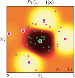
Figure 9.14 Relevance vector regression with RBF kernel. We place a prior over the dual parameters ψ that encourages sparsity. After learning, the posterior distribution over most of the parameters is tightly centered around zero and they can be dropped from the model. Large points indicate data examples associated with nonzero dual parameters. The solution here can be computed from just 6 of the 40 datapoints but nonetheless classifies the data almost as well as the full kernel approach (Figure 9.13).

9.7 Incremental fitting and boosting

In the previous section, we developed the relevance vector classification model in which we applied a prior that encourages sparsity in the dual logistic regression parameters ψ and hence encouraged the model to depend on only a subset of the training data. It is similarly possible to develop a sparse logistic regression method by placing a prior that encourages sparsity in the original parameters and hence encourages the classifier to depend only on a subset of the data dimensions. This is left as an exercise to the reader.

In this section we will investigate a different approach to inducing sparsity; we will add one parameter at a time to the model in a greedy fashion; in other words, we add the parameter that improves the objective function most at each stage and then consider this fixed. As the most discriminative parts of the model are added first, it is possible to truncate this process after only a small fraction of the parameters are added and still achieve good results. The remaining, unused parameters can be considered as having a value of zero, and so this model also provides a sparse solution. We term this approach incremental fitting. We will work with the original formulation (so that the sparsity is over the data dimensions), although these ideas can equally be adapted to the dual case.

To describe the incremental fitting procedure, let us work with the nonlinear formulation of logistic regression (Section 9.3) where the probability of the class given the data was described as

where sig[•] is the logistic sigmoid function and the activation a_i is given by

and f[•] is a nonlinear transformation that returns the transformed vector z_i.

To simplify the subsequent description, we will now write the activation term in a slightly different way so that the dot product is described explicitly as a weighted sum of individual nonlinear functions of the data

Here f[•,•] is a fixed nonlinear function that takes the data vector x_i and some parameters ξ_k and returns a scalar value. In other words, the k^th entry of the transformed vector z arises by passing the data x through the function with the k^th parameters ξ_k. Example functions f[•,•] might include :

• Arc tan functions, ξ = {α}

• Radial basis functions, ξ = {α,λ₀}

In incremental learning, we construct the activation term in Equation 9.47 piecewise. At each stage we add a new term, leaving all of the previous terms unchanged except the additive constant ₀. So, at the first stage, we use the activation

and learn the parameters ₀,₁, and ξ₁ using the maximum likelihood approach. At the second stage, we fit the function

and learn the parameters ₀,₂, and ξ₂, while keeping the remaining parameters ₁ and ξ₁ constant. At the K^th stage, we fit a model with activation

and learn the parameters ₀,_k, and ξ_K, while keeping the remaining parameters ₁…_k−1 and ξ₁…ξ_k−1 constant.

At each stage, the learning is carried out using the maximum likelihood approach. We use a nonlinear optimization procedure to maximize the log posterior probability L with respect to the relevant parameters. The derivatives required by the optimization procedure depend on the choice of nonlinear function but can be computed using the chain rule relations (Equation 9.21).

This procedure is obviously suboptimal as we do not learn the parameters together or even revisit early parameters once they have been set. However, it has three nice properties.

1. It creates sparse models: the weights _k tend to decrease as we move through the sequence, and each subsequent basis function tends to have less influence on the model. Consequently, the series can be truncated to the desired length and the associated performance is likely to remain good.

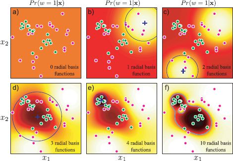
Figure 9.15 Incremental approach to fitting nonlinear logistic regression model with RBF functions. a) Before fitting, the activation (and hence the posterior probability) is uniform. b) Posterior probability after fitting one function (center and scale of RBF shown in blue). c–e) After fitting two, three, and four RBFs. e) After fitting ten RBFs. f) The data are now all classified correctly as can be seen from the decision boundary (cyan line).

2. The previous logistic regression models have been suited to cases where either the dimensionality D of the data is small (original formulation) or the number of training examples I is small (dual formulation). However, it is quite possible that neither of these things is true. A strong advantage of incremental fitting is that it is still practical when the data are high-dimensional and there are a large number of training examples. During training, we do not need to hold all of the transformed vectors z in memory at once: at the K^th stage, we need only the K^th dimension of the transformed parameters z_K = f[x, ξ_K] and the aggregate of the previous contributions to activation term Σ^K−1_{k=1 k} f[x_i,ξ_k].

3. Learning is relatively inexpensive because we only optimize a few parameters at each stage.

Figure 9.15 illustrates the incremental approach to learning a 2D data set using radial basis functions. Notice that even after only a few functions have been added to the sequence, the classification is substantially correct. Nonetheless, it is worth continuing to train this model even after the training data are classified correctly. Usually the model continues to improve and the classification performance on test data will continue to increase for some time.

9.7.1 Boosting

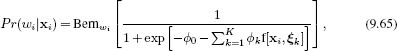
There is a special case of the incremental approach to fitting nonlinear logistic regression that is commonly used in vision applications. Consider a logistic regression model based on a sum of step functions

where the function heaviside[•] returns 0 if its argument is less than 0 and 1 otherwise. As usual, we have attached a 1 to the start of the data x so that the parameters α_k contain both a direction [α_k1,α_k2,…,α_KD] in the D-directional space (which determines the direction of the step function) and an offset α_k0 (that determines where the step occurs).

One way to think about the step functions is as weak classifiers they return 0 or 1 depending on the value of x_i so each classifies the data. The model combines these weak classifiers to compute a final strong classifier. Schemes for combining weak classifiers in this way are generically known as boosting and this particular model is called logitboost.

Unfortunately, we cannot simply fit this model using a gradient-based optimization approach because the derivative of the heaviside step function with respect to the parameters α_k is not smooth. Consequently, it is usual to predefine a large set of J weak classifiers and assume that each parameter vector α_k is taken from this set so that α_k ∈{α⁽¹⁾…α^(J)}.

As before, we learn the logitboost model incrementally by adding one term at a time to the activation (Equation 9.53). However, now we exhaustively search over the weak classifiers {α⁽¹⁾…α^(J)} and for each use nonlinear optimization to estimate the weights ₀ and _k. We choose the combination {α_k,₀,_k} that improves the log likelihood the most. This procedure may be made even more efficient (but more approximate) by choosing the weak classifier based on the log likelihood after just a single Newton or gradient descent step in the nonlinear optimization stage. When we have selected the best weak classifier α_k, we can return and perform the full optimization over the offset ₀ and weight _k.

Note that after each classifier is added, the relative importance of each datapoint is effectively changed: the datapoints contribute to the derivative according to how well they are currently predicted (Equation 9.9). Consequently, the later weak classifiers become more specialized to the more difficult parts of the data set that are not well classified by the early ones. Usually, these are close to the final decision boundary.

Figure 9.16 shows several iterations of the boosting procedure. Because the model is composed from step functions, the final classification boundary is irregular and does not interpolate smoothly between the data examples. This is a potential disadvantage of this approach. In general, a classifier based on arc tangent functions (roughly smooth step functions) will have superior generalization and can also be fit using continuous optimization. It could be argued that the step function is faster to evaluate, but even this is illusory as more complex functions such as the arc tangent can be approximated with look-up tables.

9.8 Classification trees

In the nonlinear logistic regression model, we created complex decision boundaries using an activation function that is a linear combination ^Tz of nonlinear functions z =f[x] of the data x. We now investigate an alternative method to induce complex decision boundaries: we partition data space into distinct regions and apply a different classifier in each region.

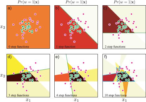
Figure 9.16 Boosting. a) We start with a uniform prediction Pr(w=1|x) and b) incrementally add a step function to the activation (green line indicates position of step). In this case the parameters of the step function were chosen greedily from a predetermined set containing 20 angles each with 40 offsets. c)-e) As subsequent functions are added the overall classification improves. f) However, the final decision surface (cyan line) is complex and does not interpolate smoothly between regions of high confidence.

The branching logistic regression model has activation,

The term g[•,•] is a gating function that returns a number between 0 and 1. If this gating function returns 0, then the activation will be ₀x_i, whereas if it returns 1, the activation will be ₁x_i. If the gating returns an intermediate value, then the activation will be a weighted sum of these two components. The gating function itself depends on the data x_i and takes parameters ω. This model induces a complex nonlinear decision boundary (Figure 9.17) where the two linear functions ₀x_i and ₁x_i are specialized to different regions of the data space. In this context, they are sometimes referred to as experts.

The gating function could take many forms, but an obvious possibility is to use a second logistic regression model. In other words, we compute a linear function ω^Tx_i of the data that is passed through a logistic sigmoid so that

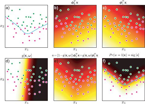
Figure 9.17 Branching logistic regression. a) This data set needs a nonlinear decision surface (cyan line) to classify the data reasonably. b) This linear activation is an expert that is specialized to describing the right-hand side of the data. c) This linear activation is an expert that describes the left-hand side of the data. d) A gating function takes the data vector x and returns a number between 0 and 1, which we will use to decide which expert contributes at each decision. e) The final activation consists of a weighted sum of the activation indicated by the two experts where the weight comes from the gating function. f) The final classifier predictions Pr(w = 1|x) are generated by passing this activation through the logistic sigmoid function.

To learn this model we maximize the log probability L = ∑_i log [Pr(w_i|x_i)] of the training data pairs {x_i,w_i}^I_i=1 with respect to all of the parameters θ = {₀,₁,ω}. As usual this can be accomplished using a nonlinear optimization procedure. The parameters can be estimated simultaneously or using a coordinate ascent approach in which we update the three sets of parameters alternately.

We can extend this idea to create a hierarchical tree structure by nesting gating functions (Figure 9.18). For example, consider the activation

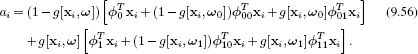
This is an example of a classification tree.

To learn the parameters θ=(₀,₁,₀₀,₀₁,₁₀,₁₁,ω,ω₀,ω₁}, we could take an incremental approach. At the first stage, we fit the top part of the tree (Equation 9.54), setting parameters ω,₀,₁. Then we fit the left branch, setting parameters ω₀,₀₀,₀₁ and subsequently the right branch, setting parameters ω₁,₁₀,₁₁, and so on.

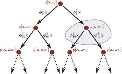
Figure 9.18 Logistic classification tree. Data flows from the root to the leaves. Each node is a gating function that weights the contributions of terms in the subbranches in the final activation. The gray region indicates variables that would be learned together in an incremental training approach.

The classification tree has the potential advantage of speed. If each gating function produces a binary output (like the heaviside step function), then each datapoint passes down just one of the outgoing edges from each node and ends up at a single leaf. When each branch in the tree is a linear operation (as in this example), these operations can be aggregated to a single linear operation at each leaf. Since each datapoint receives specialized processing, the tree need not usually be deep, and new data can be classified very efficiently.

9.9 Multiclass logistic regression

Throughout this chapter, we have discussed binary classification. We now discuss how to extend these models to handle N > 2 world states. One possibility is to build N one-against-all binary classifiers each of which computes the probability that the n^th class is present as opposed to any of the other classes. The final label is assigned according to the one-against-all classifier with the highest probability.

The one-against-all approach works in practice but is not very elegant. A more principled way to cope with multiclass classification problems is to describe the the posterior Pr(w|x) as a categorical distribution, where the parameters λ = [λ₁…λ_N] are functions of the data x

where the parameters are in the range λ_n ∈ [0, 1] and sum to one, ∑_n λ_n = 1. In constructing the function λ[x], we must ensure that we obey these constraints.

As for the two class logistic regression case, we will base the model on linear functions of the data x and pass these through a function that enforces the constraints. To this end, we define N activations (one for each class),

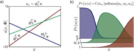
Figure 9.19 Multiclass logistic regression. a) We form one activation for each class based on linear functions of the data. b) We pass these activations through the softmax function to create the distribution Pr(w|x) which is shown here as a function of x. The softmax function takes the three real-valued activations and returns three positive values that sum to one, ensuring that the distribution Pr(w|x) is a valid probability distribution for all x.

where {_n}^N_n=1 are parameter vectors. We assume that as usual we have prepended a 1 to each of the data vectors x_i so that the first entry of each parameter vector _n represents an offset. The n^th entry of the final categorical distribution is now defined by

The function softmax[•] takes the N activations {a_n}^N_n=1, which can take any real number, and maps them to the N parameters {λ_n}^N_n=1 of the categorical distribution, which are constrained to be positive and sum to one (Figure 9.19).

To learn the parameters θ = {_n}^N_n=1 given training pairs (w_i, x_i) we optimize the log likelihood of the training data

As for the two-class case, there is no closed form expression for the maximum likelihood parameters. However, this is a convex function, and the maximum can be found using a nonlinear optimization technique such as the Newton method. These techniques require the first and second derivatives of the log likelihood with respect to the parameters, which are given by

where we define the term

It is possible to extend multiclass logistic regression in all of the ways that we extended the two-class model. We can construct Bayesian, nonlinear, dual and kernelized versions. It is possible to train incrementally and combine weak classifiers in a boosting framework. Here, we will consider tree-structured models as these are very common in modern vision applications.

9.10 Random trees, forests, and ferns

In Section 9.8 we introduced the idea of tree-structured classifiers, in which the processing for each data example is different and becomes steadily more specialized. This idea has recently become extremely popular for multiclass problems in the form of random classification trees.

As for the two-class case, the key idea is to construct a binary tree where at each node, the data are evaluated to determine whether it will pass to the left or the right branch. Unlike in Section 9.8, we will assume that each data point passes into just one branch. In a random classification tree, the data are evaluated against a function q[x] that was randomly chosen from a predefined family of possible functions. For example, this might be the response of a randomly chosen filter. The data point proceeds one way in the tree if the response of this function exceeds a threshold τ and the other way if not. While the functions are chosen randomly, the threshold is carefully selected.

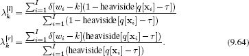
We select the threshold that maximizes the log-likelihood L of the data:

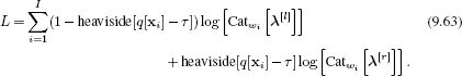
Here the first term represents the contribution of the data that passes down the left branch, and the second term represents the contribution of the data that passes down the right branch. In each case, the data are evaluated against a categorical distribution with parameters λ^[l] and λ^[r], respectively. These parameters are set using maximum likelihood:

The log likelihood is not a smooth function of the threshold τ, and so in practice we maximize the log likelihood by empirically trying a number of different threshold values and choosing the one that gives the best result.

We then perform this same procedure recursively; the data that pass to the left branch have a new randomly chosen classifier applied to them, and a new threshold that splits it again is chosen. This can be done without recourse to the data in the right branch. When we classify a new data example x*, we pass it down the tree until it reaches one of the leaves. The posterior distribution pr(w*|x*) over the world state w* is set to Cat_w*[λ] where the parameters λare the categorical parameters associated with this leaf during the training process.

The random classification tree is attractive because it is very fast to train – after all, most of its parameters are chosen randomly. It can also be trained with very large amounts of data as its complexity is linear in the number of data examples.

There are two important variations on this model:

1. A fern is a tree where the randomly chosen functions at each level of the tree are constrained to be the same. In other words, the data that pass through the left and right branches at any node are subsequently acted on by the same function (although the threshold level may optionally be different in each branch). In practice, this means that every datapoint is acted on by the same sequence of functions. This can make implementation extremely efficient when we are evaluating the classifier repeatedly.

2. A random forest is a collection of random trees, each of which uses a different randomly chosen set of functions. By averaging together the probabilities Pr(w*|x*) predicted by these trees, a more robust classifier is produced. One way to think of this is as approximating the Bayesian approach; we are constructing the final answer by taking a weighted sum of the predictions suggested by different sets of parameters.

9.11 Relation to non-probabilistic models

In this chapter, we have described a family of probabilistic algorithms for classification. Each is based on maximizing either the log Bernoulli probability of the training class labels given the data (two-class case) or the log categorical probability of the training class labels given the data (multiclass case).

However, it is more common in the computer vision literature to use non-probabilistic classification algorithms such as the multilayer perceptron, adaboost, or support vector classification. At their core, these algorithms optimize different objective functions and so are neither directly equivalent to each other, nor to the models in this chapter.

We chose to describe the less common probabilistic algorithms because

• They have no serious disadvantages relative to non-probabilistic techniques,

• They naturally produce estimates of certainty,

• They are easily extensible to the multiclass case, whereas non-probabilistic algorithms usually rely on one-against-all formulations, and

• They are more easily related to one another and to the rest of the book.

In short, it can reasonably be argued that the dominance of non-probabilistic approaches to classification is largely for historical reasons. We will now briefly describe the relationship between our models and common non-probabilistic approaches.

The multilayer perceptron (MLP) or neural network is very similar to our nonlinear logistic regression model in the special case where the nonlinear transformation consists of a set of sigmoid functions applied to linear projections of data (e.g., z_k = arctan [α^T_kx]). In the MLP, learning is known as back propagation and the transformed variable z is known as the hidden layer.

Adaboost is very closely related to the the logitboost model described in this chapter, but adaboost is not probabilistic. Performance of the two algorithms is similar.

The support vector machine (SVM) is similar to relevance vector classification; it is a kernelized classifier that depends sparsely on the data. It has the advantage that its objective function is convex, whereas the objective function in relevance vector classification is non-convex and only guarantees to converge to a local minimum. However, the SVM has several disadvantages: it does not assign certainty to its class predictions, it is not so easily extended to the multiclass case, it produces solutions that are less sparse than relevance vector classification, and it places more restrictions on the form of the kernel function. In practice, classification performance of the two models is again similar.

9.12 Applications

We now present a number of examples of the use of classification in computer vision from the research literature. In many of the examples, the method used was non-probabilistic (e.g., adaboost), but is very closely related to the algorithms in this chapter, and one would not expect the performance to differ significantly if these were substituted.

9.12.1 Gender classification

The algorithms in this chapter were motivated by the problem of gender detection in unconstrained facial images. The goal is to assign a label w ∈{0, 1} indicating whether a small patch of an image x contains a male or a female face. Prince and Aghajanian (2009) developed a system of this type. First, a bounding box around the face was identified using a face detector (see next section). The data within this bounding box were resized to 60 × 60, converted to grayscale and histogram equalized. The resulting image was convolved with a bank of Gabor functions, and the filtered images sampled at regular intervals that were proportionate to the wavelength to create a final feature vector of length 1064. Each dimension was whitened to have mean zero and unit standard deviation. Chapter 13 contains information about these and other preprocessing methods.

A training database of 32,000 examples was used to learn a nonlinear logistic regression model of the form

where the nonlinear functions f[•] were arc tangents of linear projections of the data so that

As usual the data were augmented by prepending a 1 so the projection vectors {ξ_k} were of length D + 1. This model was learned using an incremental approach so that at each stage the parameters ₀,_k and ξ_k were modified.

The system achieved 87.5 percent performance with K = 300 arc tangent functions on a challenging real-world database that contained large variations in scale, pose, lighting, and expression similar to the faces in Figure 9.1. Human observers managed only 95 percent performance on the same database using the resized face region alone.

9.12.2 Face and pedestrian detection

Before we can determine the gender of a face, we must first find it. In face detection (Figure 7.1), we assign a label w ∈{0, 1} to a small region of the image x indicating whether a face is present (w=1) or not (w=0). To ensure that the face is found, this process is repeated at every position and scale in the image and consequently the classifier must be very fast.

Viola and Jones (2004) presented a face detection system based on adaboost (Figure 9.20). This is a non-probabilistic analogue of the boosting methods described in Section 9.7.1. The final classification is based on the sign of a sum of nonlinear functions of the data

where the nonlinear functions f[•] are heaviside step functions of projections of the data (weak classifiers giving a response of zero or one for each possible data vector x) so that

As usual, the data vector x was prepended with a 1 to account for an offset.

The system was trained on 5,000 faces and 10,000 non-face regions, each of which were represented as a 24 × 24 image patch. Since the model is not smooth (due to the step function) gradient-based optimization is unsuitable, and so Viola and Jones (2004) exhaustively searched through a very large number of predefined projections ξ_k.

There were two aspects of the design that ensured that the system ran quickly.

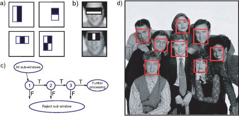
Figure 9.20 Fast face detection using a boosting method (viola and Jones 2004). a) Each weak classifier consists of the response of the image to a Haar filter, which is then passed through a step function. b) The first two weak classifiers learned in this implementation have clear interpretations: The first responds to the dark horizontal region belonging to the eyes, and the second responds to the relative brightness of the bridge of the nose. c) The data passes through a cascade: most regions can be quickly rejected after evaluating only a few weak classifiers as they look nothing like faces. More ambiguous regions undergo further preprocessing. d) Example results. Adapted viola and Jones (2004).

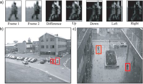
Figure 9.21 Boosting methods based on the thresholded responses of Haar functions have also been used for pedestrian detection in video footage. a) To improve detection rates two subsequent frames are used. The absolute difference between the frames is computed as is the difference when one of the frames is offset in each of four directions. The set of potential weak classifiers consists of Haar functions applied to all of these representations. b,c) Example results. Adapted from viola et al. (2005). ©2005 Springer.

1. The structure of the classifier was exploited: training in boosting is incremental – the “weak classifiers” (nonlinear functions of the data) are incrementally added to create an increasingly sophisticated strong classifier. Viola and Jones (2004) exploited this structure when they ran the classifier: they reject regions that are very unlikely to be faces based on responses of the first few weak classifiers and only subject more ambiguous regions to further processing. This is known as a cascade structure. During training, the later stages of the cascade are trained with new negative examples that were not rejected by the earlier stages.

2. The projections ξ_k were carefully chosen so that they were very fast to evaluate: they consisted of Haar-like filters (Section 13.1.3), which require only a few operations to compute.

The final system consisted of 4297 weak classifiers divided into a 32-stage cascade. It found 91.1 percent of 507 frontal faces across 130 images, with a false positive rate of less than 1 per frame, and processed images in fractions of a second.

Viola et al. (2005) developed a similar system for detecting pedestrians in video sequences (Figure 9.21). The main modification was to extend the set of weak classifiers to encompass features that span more than one frame and hence select for the particular temporal patterns associated with human motion. To this end their system used not only the image data itself, but also the difference image between adjacent frames and similar difference images when taken after offsetting the frames in each of four directions. The final system achieved an 80 percent detection rate with a false alarm rate of 1/400,000 which corresponds to one false positive for every two frames.

9.12.3 Semantic segmentation

The goal of semantic segmentation is to assign a label w ∈{1… M} to each pixel indicating which of M objects is present, based on the local image data x. Shotton et al. (2009) developed a system known as textonboost that was based on a non-probabilistic boosting algorithm called jointboost (Torralba et al. 2007). The decision was based on a one-against-all strategy in which M binary classifiers are computed based on the weighted sums

where the nonlinear functions f[•] were once more based on heaviside step functions. Note that the weighted sums associated with each object class share the same nonlinear functions but weight them differently. After computing these series, the decision is assigned based on the activation a_m that is the greatest.

Shotton et al. (2009) based the nonlinear functions on a texton representation of the image: each pixel in the image is replaced by a discrete index indicating the “type” of texture present at that position (see Section 13.1.5). Each nonlinear function considers one of these texton types and computes the number of times that it is found within a rectangular area. This area has a fixed spatial displacement from the pixel under consideration (Figures 9.22c–f). If this displacement is zero, then the function provides evidence about the pixel directly (e.g., it looks like grass). If the spatial displacement is larger, then the function provides evidence of the local context (e.g., there is grass nearby, so this pixel may belong to a cow).

For each nonlinear function, an offset is added to the texton count and the result is passed through a step function. The system was learned incrementally by assessing each of a set of a randomly chosen classifiers (defined by the choice of texton, rectangular region, and offset) and choosing the best at the current stage.

The full system also included a postprocessing step in which the result was refined using a conditional random field model (see Chapter 12). It achieved 72.2 percent performance on the challenging MRSC database that includes 21 diverse object classes including wiry objects such as bicycles and objects with a large degree of variation such as dogs.

9.12.4 Recovering surface layout

To recover the surface layout of a scene we assign a label w ∈{1…3} to each pixel in the image indicating whether the pixel contains a support object (e.g., floor), a vertical object (e.g., building), or the sky. This decision is based on local image data x. Hoiem et al. (2007) constructed a system of this type using a one-against-all principle. Each of the three binary classifiers was based on logitboosted classification trees; different classification trees are treated as weak classifiers, and the results are weighted together to compute the final probability.

Hoeim et al. (2007) worked with the intermediate representation of superpixels – an oversegmentation of the scene into small homogeneous regions, which are assumed to belong to the same object. Each superpixel was assigned a label w using the classifier based on a data vector x, which contained location, appearance, texture, and perspective information associated with the superpixel.

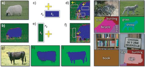
Figure 9.22 Semantic image labeling using “TextonBoost.” a) Original image. b) Image converted to textons – a discrete value at each pixel indicating the type of texture that is present. c) The system was based on weak classifiers that count the number of textons of a certain type within a rectangle that is offset from the current position (yellow cross). d) This provides both information about the object itself (contains sheep-like textons) and nearby objects (near to grass-like textons). e,f) Another example of a weak classifier. g) Test image. h) Per-pixel classification is not very precise at the edges of objects and so i) a conditional random field is used to improve the result. j) Examples of results and ground truth. Adapted from shotton et al. 2009). ©2009 Springer.

To mitigate against the possibility that the original superpixel segmentation was wrong, multiple segmentations were computed and the results merged to provide a final per-pixel classification (Figure 9.23). In the full system, regions that were classified as vertical were subclassified into left-facing planar surfaces, frontoparallel planar surfaces, or right-facing planar surfaces or nonplanar surfaces, which may be porous (e.g., trees) or solid. The system was trained and tested on a data set consisting of images collected from the Web including diverse environments (forests, cities, roads, etc.) and conditions (snowy, sunny, cloudy, etc.). The data set was pruned to remove photos where the horizon was not within the image.

The system correctly labeled 88.1 percent of pixels correctly with respect to the main three classes and 61.5 percent correctly with respect to the subclasses of the vertical surface. This algorithm was the basis of a remarkable system for creating a 3D model from a single 2D photograph (Hoeim et al. 2005).

9.12.5 Identifying human parts

Shotton et al. (2011) describe a system that assigns a discrete label w ∈ {1,…,31}, indicating which of 31 body parts is present at each pixel based on a depth image x. The resulting distribution of labels is an intermediate representation in a system that proposes a possible configuration of the 3D joint positions in the Microsoft Kinect gaming system (Figure 9.24).

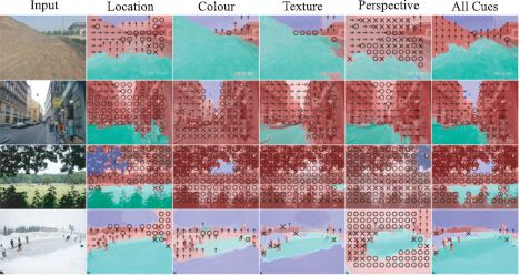
Figure 9.23 Recovering surface layout. The goal is to take an image and return a label indicating whether the pixel is part of a support surface (green pixels) vertical surface (red pixels) or the sky (blue pixels). Vertical surfaces were subclassified into planar objects at different orientations (left arrows, upward arrows and right arrows denote left-facing, frontoparrallel and right-facing surfaces) and nonplanar objects which can be porous (marked as “o”) or nonporous (marked as “x”. The final classification was based on (i) location cues (which include position in the image and position relative to the horizon), (ii) color cues, (iii) texture cues, and (iv) perspective cues which were based on the statistics of line segments in the region. The figure shows example classifications for each of these cues alone and when combined. Adapted from Hoiem et al(2007). ©2007 Springer.

The classification was based on a forest of decision trees: the final probability Pr(w|x) is an average (i.e., a mixture) of the predictions from a number of different classification trees. The goal is to mitigate against biases introduced by the greedy method with which a single tree is trained.

Within each tree, the decision about which branch a datapoint travels down is based on the difference in measured depths at two points, each of which is spatially offset from the current pixel. The offsets are inversely scaled by the distance to the pixel itself, which ensures that they address the same relative positions on the body when the person moves closer or further away to the depth camera.

The system was trained from a very large data set of 900,000 depth images, which were synthesized based on motion capture data and consisted of three trees of depth 20. Remarkably, the system is capable of assigning the correct label 59 percent of the time, and this provides a very solid basis for the subsequent joint proposals.

Discussion

In this chapter we have considered classification problems. We note that all of the ideas that were applied to regression models in Chapter 8 are also applicable to classification problems. However, for classification the model includes a nonlinear mapping between the data x and the parameters of the distribution Pr(w|x) over the world w. This means that we cannot find the maximum likelihood solution in closed form (although the problem is still convex) and we cannot compute a full Bayesian solution without making approximations.

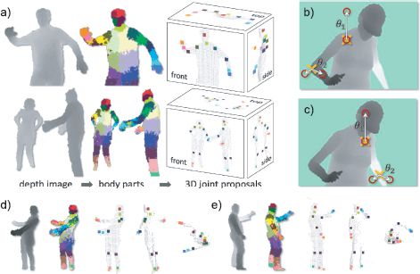
Figure 9.24 Identifying human parts. a) The goal of the system is to take a depth image x and assign a discrete label w to each pixel indicating which of 31 possible body parts is present. These depth labels are used to form proposals about the position of 3D joints. b) The classification is based on decision trees. At each point in the tree, the data are divided according to the relative depth at two points (red circles) offset relative to the current pixel (yellow crosses). In this example, this difference is large in both cases, whereas in c) this difference is small – hence these differences provide information about the pose. d,e) Two more examples of depth image, labeling and hypothesized pose. Adapted from Shotton et al. (2011). ©2011 IEEE.

Classification techniques have many uses in machine vision. Notice though that these models have no domain-specific information about the problem other than that provided by the preprocessing of the data. This is both an advantage (they find many applications) and a disadvantage (they cannot take advantage of a priori information about the problem). In the remaining part of the book we will explore models that introduce increasing amounts of domain-specific information to the problem.

Notes

Classification in vision: Classification techniques such as those discussed in this chapter have been applied to many problems in vision including face detection (Viola and Jones 2004), surface layout estimation creation (Hoiem et al. 2007), boundary detection (Dollár et al. 2006), keypoint matching (Lepetit et al. 2005), body part classification (Hoiem et al. 2007), semantic segmentation (He et al. 2004), object recognition (Csurka et al. 2004), and gender classification (Kumar et al. 2008).

Probabilistic classification: More information about logistic regression can be found in Bishop(2006) and many other statistics textbooks. Kernel logistic regression (or Gaussian process regression) was presented in Williams and Barbar (1998) and more information can be found in Rasmussen and Williams (2006). A sparse version of kernel logistic regression (relevance vector classification) was presented by Tipping (2001) and a sparse multiclass variant was developed by Brishnapuram et al. (2005). Probabilistic interpretations of boosting were introduced by Friedman et al. (2000). Random forests of multinomial regressors were introduced in Prinzie and Van Den Poel (2008).

Other classification schemes: In this chapter, we have presented a family of probabilistic classification models based on logistic regression. There are other non-probabilistic techniques for classification, and these include single and multilayer perceptrons Rosenblatt 1958; Rumelhart et al. 1986), support vector machines (Vapnik 1995; Cristianini and Shawe-Taylor 2000), and adaboost (Freund and Schapire 1995). A critical difference between these techniques is the underlying objective function. Logistic regression models optimize the log Bernoulli probability, but the other models optimize different criteria, such as the hinge loss (support vector machines) or exponential error (adaboost). It is difficult to make general statements about the relative merits of these approaches, but it is probably fair to say that (i) there is no major disadvantage to using the probabilistic techniques in this chapter and (ii) the choice of classification method is usually less important in vision problems than the preprocessing of the data. Methods based on boosting and classification trees are particularly popular in vision because of their speed.

Boosting: Adaboost was introduced by Freund and Schapire (1995). Since then there have been a large number of variations, most of which have been used in computer vision. These include discrete adaboost (Freund and schapire 1996), real adaboost (Schapire and Singer 1998), gentleboost (Friedman et al. 2000), logitboost (Friedman et al. 2000), floatboost (Li er al.2003), KLBoost (Liu and Shum 2003), asymmetric boost (Viola and Jonse 2002), and statboost (Pham and Cham 2007a). Boosting has also been applied to the multiclass case (Schapire and Singer 1998; Torralba et al. 2007) and for regression (Friedman 1999). A review of boosting approaches can be found in Meir and Mätsch (2003).

Classification trees: Classification trees have a long history in computer vision, dating back to at least Shepherd(1983). Modern interest was stimulated by Aamit and German (1997) and Breiman (2001) who investigated the use of random forests. Since this time classification trees and forests have been applied to keypoint matching (Lepetit et al. 2005), segmentation (Yin et al. 2007), human pose detection (Rogez et al. 2006; Shotton et al. 2011), object detection (Bosch et al. 2007), image classification (Moosmann et al. 2006, 2008), deciding algorithm suitability (Mac Aodha et al., 2010), detection occlusions (Humayun et al. 2011), and semantic image segmentation (Shotton et al. 2009).

Gender classification: Automatic determination of gender from a facial image has variously been tackled with neural networks (Golomb et al. 1990), support vector machines (Moghaddam and Yang 2002), linear discriminant analysis (Bekios-calfa et al. 2011) and both adaboost (Baluja and Rowley 2003), and logitboost (Prince and Aghajanaian 2009). A review is provided by Mäkinen and Raosamo (2008b) and quantative comparisons are presented in Mäkinen and Raisamo (2008a). Representative examples of the state of the art can be found in Kumar et al. (2008) and Shan (2012).

Face detection: The application of boosting to face detection (Viola and Jones 2004) usurped earlier techniques (e.g., Osuna et al. 1997, Schneiderman and Kanade 2000). Since then, many boosting variants have been applied to the problem including floatboost (Li et al. 2002; Li and Zhang 2004), gentleboost (Lienhart et al. 2003), realboost (Huang et al 2007a; Wu et al. 2007), asymboost (Pham and Cham 2007b; Viola and Jones 2002), and statboost (Pham and Cham 2007a). A recent review of this area can be found in Zhang and Zhang (2010).

Semantic segmentation: The authors of the system described in the text (Shotton et al. 2008b) subsequently presented a much faster system based on classification trees (Shotton et al. 2009). A recent comparison of quantitative performance can be found in Ranganathan (2009). Other work has investigated the imposition of prior knowledge such as the copresence of object classes (He et al. 2006) and likely spatial configurations of objects (He et al. 2004).

Problems

9.1 The logistic sigmoid function is defined as

Show that (i) sig[− ∞] = 0, (ii) sig[0] = 0.5, sig[∞]=1.

9.2 Show that the derivative of the log posterior probability for the logistic regression model

with respect to the parameters is given by

9.3 Show that the second derivatives of the log likelihood of the logistic regression model is given by

9.4 Consider fitting a logistic regression model to 1D data x where the two classes are perfectly separable. For example, perhaps all the data x where the world state w = 0 takes values less than 0 and all the data x where the world state is w = 1 takes values greater than 1. Hence it is possible to classify the training data perfectly. What will happen to the parameters of the model during learning? How could you rectify this problem?

9.5 Compute the Laplace approximation to a beta distribution with parameters α = 1.0, β = 1.0.

9.6 Show that the Laplace approximation to a univariate normal distribution with mean μ and variance σ² is the normal distribution itself.

9.7 Devise a method to choose the scale parameter λ₀ in the radial basis function in kernel logistic regression (Equation 9.33).

9.8 A mixture of experts (Jordan and Jacobs 1994) divides space into different regions, each of which receives specialized attention (Figure 9.25). For example, we could describe the data as a mixture of logistic classifiers so that

Each logistic classifier is considered as an expert and the mixing weights decide the combination of experts that are applied to the data. The mixing weights, which are positive and sum to one, depend on the data x: for a two-component model, they could be based on a second logistic regression model with activation ω^T x. This model can be expressed as the marginalization of a joint distribution between w_i and a hidden variable h_i so that

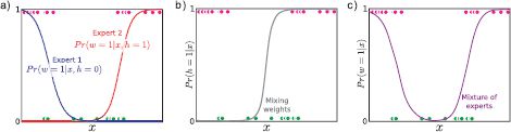
Figure 9.25 Mixture of two experts model for 1D data. Pink circles indicate positive examples. Green circles indicate negative examples. a) Two expert is specialized to model the left and right sides of the data respectively. b) The mixing weights change as a function of the data. c) The final output of the model is mixture of the two constituent experts and fits the data well.

where

How does this model differ from branching logistic regression (Section 9.8)? Devise a learning algorithm for this model.

9.9 The softmax[•,•,…,•] function is defined to return a multivariate quantity where the k^th element is given by

Show that 0 < s_k < 1 and that ∑^K_k=1 s_k = 1.

9.10 Show that the first derivative of the log-probability of the multiclass logistic regression model is given by Equation 9.61.

9.11 The classifiers in this chapter have all been based on continuous data x. Devise a model that can distinguish between M world states w ∈ {1…M} based on a discrete observation x ∈ {1…K} and discuss potential learning algorithms.

¹Note that these are the gradient and Hessian of the log likelihood that we aim to maximize. If this is implemented using a nonlinear minimization algorithm, we should multiply the objective function, gradient and Hessian by – 1.