Computer Vision: Models, Learning, and Inference (2012)
Part II
Machine learning for machine vision
Chapter 8
Regression models
This chapter concerns regression problems: the goal is to estimate a univariate world state w based on observed measurements x. The discussion is limited to discriminative methods in which the distribution Pr(w|x) of the world state is directly modeled. This contrasts with Chapter 7 where the focus was on generative models in which the likelihood Pr(x|w) of the observations is modeled.
To motivate the regression problem, consider body pose estimation: here the goal is to estimate the joint angles of a human body, based on an observed image of the person in an unknown pose (Figure 8.1). Such an analysis could form the first step toward activity recognition.
We assume that the image has already been preprocessed and a low-dimensional vector x that represents the shape of the contour has been extracted. Our goal is to use this data vector to predict a second vector containing the joint angles for each of the major body joints. In practice, we will estimate each joint angle separately; we can hence concentrate our discussion on how to estimate a univariate quantity w from continuous observed data x. We begin by assuming that the relation between the world and the data is linear and that the uncertainty around this prediction is normally distributed with constant variance. This is the linear regression model.
8.1 Linear regression
The goal of linear regression is to predict the posterior distribution Pr(w|x) over the world state w based on observed data x. Since this is a discriminative model, we proceed by choosing a probability distribution over the world w and making the parameters dependent on the data x. The world state w is univariate and continuous and so a suitable distribution is the univariate normal. In linear regression (Figure 8.2), we make the mean μ of this normal distribution a linear function ![]() 0 +
0 + ![]() T xi of the data and treat the variance σ2 as a constant so that
T xi of the data and treat the variance σ2 as a constant so that
![]()
where θ = {![]() 0,
0,![]() ,σ2} are the model parameters. The term
,σ2} are the model parameters. The term ![]() 0 can be interpreted as the y-intercept of a hyperplane and the entries of
0 can be interpreted as the y-intercept of a hyperplane and the entries of ![]() = [
= [![]() 1,
1,![]() 2,…,
2,…,![]() D]T are its gradients with respect to each of the D data dimensions.
D]T are its gradients with respect to each of the D data dimensions.
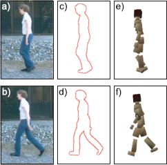
Figure 8.1 Body pose estimation. a–b) Human beings in unknown poses. c–d) The silhouette is found by segmenting the image and the contour extracted by tracing around the edge of the silhouette. A 100 dimensional measurement vector x is extracted that describes the contour shape based on the shape context descriptor (see Section 13.3.5). e–f) The goal is to estimate the vector w containing the major joint angles of the body. This is a regression problem as each element of the world state w is continuous. Adapted from Agarwal and Triggs (2006).
It is cumbersome to treat the y-intercept separately from the gradients, so we apply a trick that allows us to simplify the subsequent notation. We attach a 1 to the start of every data vector xi ← [1 xTi]T and attach the y-intercept ![]() 0to the start of the gradient vector
0to the start of the gradient vector ![]() ←[
←[![]() 0
0 ![]() T]T so that we can now equivalently write
T]T so that we can now equivalently write
![]()
In fact, since each training data example is considered independent, we can write the probability Pr(w|X) of the entire training set as a single normal distribution with a diagonal covariance so that
![]()
where X = [x1, x2,…, xI] and w = [w1, w2,…, wI]T.
Inference for this model is very simple: for a new datum x* we simply evaluate Equation 8.2 to find the posterior distribution Pr(w*|x*) over the world state w*. Hence we turn our main focus to learning.
8.1.1 Learning
The learning algorithm estimates the model parameters θ ={![]() ,σ2} from paired training examples {xi, wi}Ii=1. In the maximum likelihood approach we seek
,σ2} from paired training examples {xi, wi}Ii=1. In the maximum likelihood approach we seek
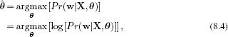
where as usual we have taken the logarithm of the criterion. The logarithm is a monotonic transformation, and so it does not change the position of the maximum, but the resulting cost function is easier to optimize. Substituting in we find that
![]()
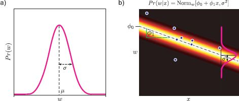
Figure 8.2 Linear regression model with univariate data x. a) We choose a univariate normal distribution over the world state w. b) The parameters of this distribution are now made to depend on the data x: the mean μ is a linear function ![]() 0 +
0 + ![]() 1 x of the data and the variance σ2 is constant. The parameters
1 x of the data and the variance σ2 is constant. The parameters ![]() 0and
0and ![]() 1 represent the intercept and slope of the linear function, respectively.
1 represent the intercept and slope of the linear function, respectively.
We now take the derivatives with respect to ![]() and σ2, equate the resulting expressions to zero and solve to find
and σ2, equate the resulting expressions to zero and solve to find
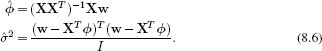
Figure 8.2b shows an example fit with univariate data x. In this case, the model describes the data reasonably well.
8.1.2 Problems with the linear regression model
There are three main limitations of the linear regression model.
• The predictions of the model are overconfident; for example, small changes in the estimated slope ![]() 1 make increasingly large changes in the predictions as we move further from the y-intercept
1 make increasingly large changes in the predictions as we move further from the y-intercept ![]() 0. However, this increasing uncertainty is not reflected in the posterior distribution.
0. However, this increasing uncertainty is not reflected in the posterior distribution.
• We are limited to linear functions and usually there is no particular reason that the visual data and world state should be linearly related.
• When the observed data x is high-dimensional, it may be that many elements of this variable aren’t useful for predicting the state of the world, and so the resulting model is unnecessarily complex.
We tackle each of these problems in turn. In the following section we address the overconfidence of the model by developing a Bayesian approach to the same problem. In Section 8.3, we generalize this model to fit nonlinear functions. In section 8.6, we introduce a sparse version of the regression model where most of the weighting coefficients ![]() are encouraged to be zero. The relationships between the models in this chapter are indicated in Figure 8.3.
are encouraged to be zero. The relationships between the models in this chapter are indicated in Figure 8.3.
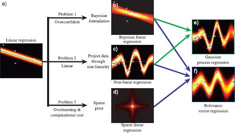
Figure 8.3 Family of regression models. There are several limitations to linear regression which we deal with in subsequent sections. The linear regression model with maximum likelihood learning is overconfident, and hence we develop a Bayesian version. It is unrealistic to always assume a linear relationship between the data and the world and to this end, we introduce a nonlinear version. The linear regression model has many parameters when the data dimension is high, and hence we consider a sparse version of the model. The ideas of Bayesian estimation, nonlinear functions and sparsity are variously combined to form the Gaussian process regression and relevance vector regression model.
8.2 Bayesian linear regression
In the Bayesian approach, we compute a probability distribution over possible values of the parameters ![]() (we will assume for now that σ2 is known, see Section 8.2.2). When we evaluate the probability of new data, we take a weighted average of the predictions induced by the different possible values.
(we will assume for now that σ2 is known, see Section 8.2.2). When we evaluate the probability of new data, we take a weighted average of the predictions induced by the different possible values.
Since the gradient vector ![]() is multivariate and continuous, we model the prior Pr(
is multivariate and continuous, we model the prior Pr(![]() ) as normal with zero mean and spherical covariance,
) as normal with zero mean and spherical covariance,
![]()
where σ2p scales the prior covariance and I is the identity matrix. Typically σ2p is set to a large value to reflect the fact that our prior knowledge is weak.
Given paired training examples {xi,wi}Ii=1, the posterior distribution over the parameters can be computed using Bayes’ rule
![]()
where, as before, the likelihood is given by
![]()
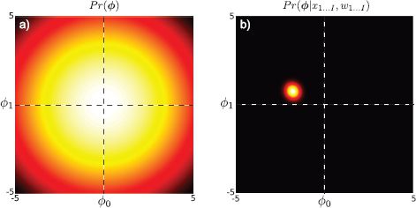
Figure 8.4 Bayesian linear regression. a) Prior Pr(![]() ) over intercept
) over intercept ![]() 0 and slope
0 and slope ![]() 1 parameters. This represents our knowledge about the parameters before we observe the data. b) Posterior distribution Pr(
1 parameters. This represents our knowledge about the parameters before we observe the data. b) Posterior distribution Pr(![]() |X, w) over intercept and slope parameters. This represents our knowledge about the parameters after observing the data from Figure 8.2b: we are considerably more certain but there remain a range of possible parameter values.
|X, w) over intercept and slope parameters. This represents our knowledge about the parameters after observing the data from Figure 8.2b: we are considerably more certain but there remain a range of possible parameter values.
The posterior distribution can be computed in closed form (using the relations in Sections 5.7 and 5.6) and is given by the expression:
![]()
where
![]()
Note that the posterior distribution Pr(![]() |X,w) is always narrower than the prior distribution Pr(
|X,w) is always narrower than the prior distribution Pr(![]() )(Figure 8.4); the data provides information that refines our knowledge of the parameter values.
)(Figure 8.4); the data provides information that refines our knowledge of the parameter values.
We now turn to the problem of computing the predictive distribution over the world state w* for a new observed data vector x*. We take an infinite weighted sum (i.e., an integral) over the predictions Pr(w*|x*,![]() ) implied by each possible
) implied by each possible ![]() where the weights are given by the posterior distribution Pr(
where the weights are given by the posterior distribution Pr(![]() |X,w).
|X,w).
To compute this, we reformulated the integrand using the relations from Sections 5.7 and 5.6 as the product of a normal distribution in ![]() and a constant with respect to
and a constant with respect to ![]() . The integral of the normal distribution must be one, and so the final result is just the constant. This constant is itself a normal distribution in w*.
. The integral of the normal distribution must be one, and so the final result is just the constant. This constant is itself a normal distribution in w*.
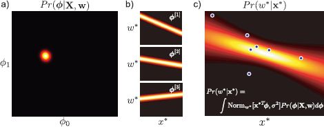
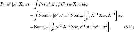
Figure 8.5 Bayesian linear regression. a) In learning we compute the posterior distribution Pr(![]() |X,w) over the intercept and slope parameters: there is a family of parameter settings that are compatible with the data. b) Three samples from the posterior, each of which corresponds to a different regression line. c) To form the predictive distribution we take an infinite weighted sum (integral) of the predictions from all of the possible parameter settings, where the weight is given by the posterior probability. The individual predictions vary more as we move from the centroid
|X,w) over the intercept and slope parameters: there is a family of parameter settings that are compatible with the data. b) Three samples from the posterior, each of which corresponds to a different regression line. c) To form the predictive distribution we take an infinite weighted sum (integral) of the predictions from all of the possible parameter settings, where the weight is given by the posterior probability. The individual predictions vary more as we move from the centroid ![]() and this is reflected in the fact that the certainty is lower on either side of the plot.
and this is reflected in the fact that the certainty is lower on either side of the plot.
This Bayesian formulation of linear regression (Figure 8.5) is less confident about its predictions, and the confidence decreases as the test data x* departs from the mean ![]() of the observed data. This is because uncertainty in the gradient causes increasing uncertainty in the predictions as we move further away from the bulk of the data. This agrees with our intuitions: predictions ought to become less confident as we extrapolate further from the data.
of the observed data. This is because uncertainty in the gradient causes increasing uncertainty in the predictions as we move further away from the bulk of the data. This agrees with our intuitions: predictions ought to become less confident as we extrapolate further from the data.
8.2.1 Practical concerns
To implement this model we must compute the D × D matrix inverse A−1 (Equation 8.12). If the dimension D of the original data is large, then it will be difficult to compute this inverse directly.
Fortunately, the structure of A is such that it can be inverted far more efficiently. We exploit the Woodbury identity (see Appendix C.8.4), to rewrite A−1 as
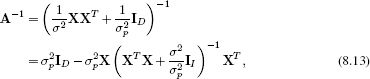
where we have explicitly noted the dimensionality of each of the identity matrices I as a subscript. This expression still includes an inversion, but now it is of size I × I where I is the number of examples: if the number of data examples I is smaller than the data dimensionality D, then this formulation is more practical. This formulation also demonstrates clearly that the posterior covariance is less than the prior; the posterior covariance is the prior covariance σp2I with a data-dependent term subtracted from it.
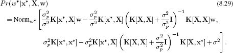
Substituting the new expression for A−1 into Equation 8.12, we derive a new expression for the predictive distribution,
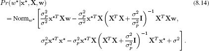
It is notable that only inner products of the data vectors (e.g., in the terms XT x*, or XTX) are required to compute this expression. We will exploit this fact when we generalize these ideas to nonlinear regression (Section 8.3).
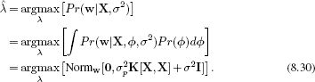
8.2.2 Fitting the variance
The previous analysis has concentrated exclusively on the slope parameters ![]() . In principle, we could have taken a Bayesian approach to estimating the variance parameter σ2 as well. However, for simplicity we will compute a point estimate of σ2 using the maximum likelihood approach. To this end, we optimize the marginal likelihood, which is the likelihood after marginalizing out
. In principle, we could have taken a Bayesian approach to estimating the variance parameter σ2 as well. However, for simplicity we will compute a point estimate of σ2 using the maximum likelihood approach. To this end, we optimize the marginal likelihood, which is the likelihood after marginalizing out ![]() and is given by
and is given by
where the integral was solved using the same technique as that used in equation 8.12.
To estimate the variance, we maximize the log of this expression with respect to σ2. Since the unknown is a scalar it is straightforward to optimize this function by simply evaluating the function over a range of values and choosing the maximum. Alternatively, we could use a general purpose nonlinear optimization technique (see Appendix B).
8.3 Nonlinear regression
It is unrealistic to assume that there is always a linear relationship between the world state w and the input data x. In developing an approach to nonlinear regression, we would like to retain the mathematical convenience of the linear model while extending the class of functions that can be described.
Consequently, the approach that we describe is extremely simple: we first pass each data example through a nonlinear transformation
![]()
to create a new data vector zi which is usually higher dimensional than the original data. Then we proceed as before: we describe the mean of the posterior distribution Pr(wi|xi) as a linear function ![]() Tzi of the transformed measurements so that
Tzi of the transformed measurements so that
![]()
For example, consider the case of 1D polynomial regression:
![]()
This model can be considered as computing the nonlinear transformation
and so it has the general form of Equation 8.17.
8.3.1 Maximum likelihood
To find the maximum likelihood solution for the gradient vector, we first combine all of the transformed training data relations (Equation 8.17) into a single expression:
![]()
The optimal weights can now be computed as
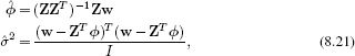
where the matrix Z contains the transformed vectors {zi}Ii=1 in its columns. These equations were derived by replacing the original data term X by the transformed data Z in the equivalent linear expressions (Equation 8.6). For a new observed data example x*, we compute the vector z* and then evaluate Equation 8.17.
Figures 8.6 and 8.7 provide two more examples of this approach. In Figure 8.6, the new vector z is computed by evaluating the data x under a set of radial basis functions:
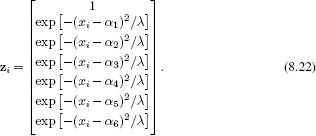
The term radial basis functions can be used to denote any spherically symmetric function, and here we have used the Gaussian. The parameters {αk}Kk=1 are the centers of the functions, and λ is a scaling factor that determines their width. The functions themselves are shown in Figure 8.6b. Because they are spatially localized, each one accounts for a part of the original data space. We can approximate a function by taking weighted sums ![]() Tz of these functions. For example, when they are weighted as in Figure 8.6c, they create the function in Figure 8.6a.
Tz of these functions. For example, when they are weighted as in Figure 8.6c, they create the function in Figure 8.6a.
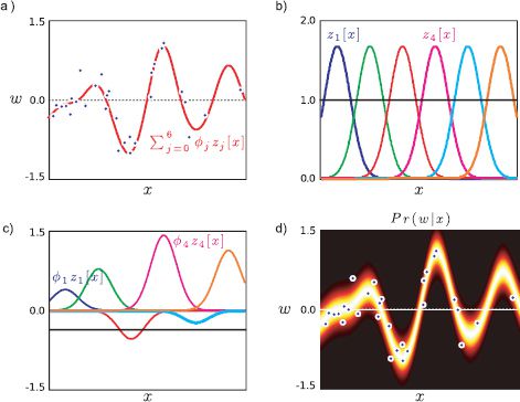
Figure 8.6 Nonlinear regression using radial basis functions. a) The relationship between the data x and world w is clearly not linear. b) We compute a new seven-dimensional vector z by evaluating the original observation x against each of six radial basis functions (Gaussians) and a constant function (black line). c) The mean of the predictive distribution (red line in (a)) can be formed by taking a linear sum ![]() Tz of these seven functions where the weights are as shown. The weights are estimated by maximum likelihood estimation of the linear regression model using the nonlinearly transformed data z instead of the original data x. d) The final distribution Pr(w|x) has a mean that is a sum of these functions and constant variance σ2.
Tz of these seven functions where the weights are as shown. The weights are estimated by maximum likelihood estimation of the linear regression model using the nonlinearly transformed data z instead of the original data x. d) The final distribution Pr(w|x) has a mean that is a sum of these functions and constant variance σ2.
In Figure 8.7 we compute a different nonlinear transformation and regress against the same data. This time, the transformation is based on arc tangent functions so that
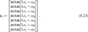
Here, the parameter λ controls the speed with which the function changes and the parameters {αm}7m=1 determine the horizontal offsets of the arc tangent functions.
In this case, it is harder to understand the role of each weighted arc tangent function in the final regression, but nonetheless they collectively approximate the function well.
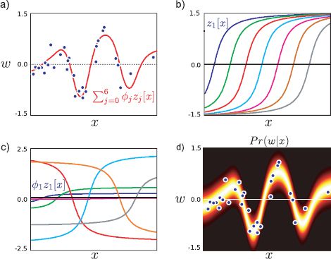
Figure 8.7 Nonlinear regression using arc tangent functions. a) The relationship between the data x and world w is not linear. b) We compute a new seven-dimensional vector z by evaluating the original observation x against each of seven arc tangent functions. c) The mean of the predictive distribution (red line in (a)) can be formed by taking a linear sum of these seven functions weighted as shown. The optimal weights were established using the maximum likelihood approach. d) The final distribution Pr(w|x) has a mean that is a sum of these weighted functions and constant variance.
8.3.2 Bayesian nonlinear regression
In the Bayesian solution, the weights ![]() of the nonlinear basis functions are treated as uncertain: in learning we compute the posterior distribution over these weights. For a new observation x*, we compute the transformed vector z* and compute an infinite weighted sum over the predictions due to the possible parameter values (Figure 8.8). The new expression for the predictive distribution is
of the nonlinear basis functions are treated as uncertain: in learning we compute the posterior distribution over these weights. For a new observation x*, we compute the transformed vector z* and compute an infinite weighted sum over the predictions due to the possible parameter values (Figure 8.8). The new expression for the predictive distribution is
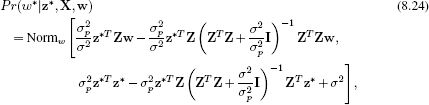
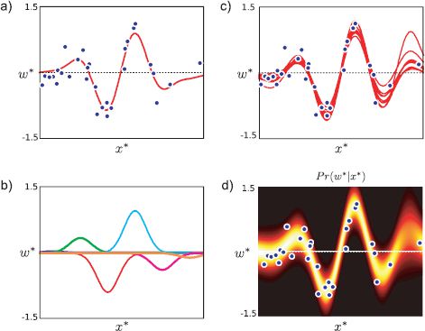
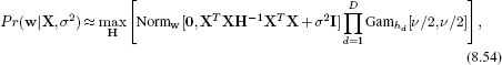
Figure 8.8 Bayesian nonlinear regression using radial basis functions. a) The relationship between the data and measurements is nonlinear. b) As in Figure 8.6, the mean of the predictive distribution is constructed as a weighted linear sum of radial basis functions. However, in the Bayesian approach we compute the posterior distribution over the weights ![]() of these basis functions. c) Different draws from this distribution of weight parameters result in different predictions. d) The final predictive distribution is formed from an infinite weighted average of these predictions where the weight is given by the posterior probability. The variance of the predictive distribution depends on both the mutual agreement of these predictions and the uncertainty due to the noise term σ2. The uncertainty is greatest in the region on the right where there is little data and so the individual predictions vary widely.
of these basis functions. c) Different draws from this distribution of weight parameters result in different predictions. d) The final predictive distribution is formed from an infinite weighted average of these predictions where the weight is given by the posterior probability. The variance of the predictive distribution depends on both the mutual agreement of these predictions and the uncertainty due to the noise term σ2. The uncertainty is greatest in the region on the right where there is little data and so the individual predictions vary widely.
where we have simply substituted the transformed vectors z for the original data x in Equation 8.14. The prediction variance depends on both the uncertainty in ![]() and the additive variance σ2. The Bayesian solution is less confident than the maximum likelihood solution (compare Figures 8.8d and 8.7d), especially in regions where the data is sparse.
and the additive variance σ2. The Bayesian solution is less confident than the maximum likelihood solution (compare Figures 8.8d and 8.7d), especially in regions where the data is sparse.
To compute the additive variance σ2 we again optimize the marginal likelihood. The expression for this can be found by substituting Z for X in Equation 8.15.
8.4 Kernels and the kernel trick
The Bayesian approach to nonlinear regression described in the previous section is rarely used directly in practice: the final expression for the predictive distribution (Equation 8.24) relies on computing inner products ziT zj. However, when the transformed space is high-dimensional, it may be costly to compute the vectors zi = f[xi] and zj = f[xj] explicitly and then compute the inner product ziT zj.
An alternative approach is to use kernel substitution in which we directly define a single kernel function k[xi,xj] as a replacement for the operation f[xi]T f[xj]. For many transformations f[•], it is more efficient to evaluate the kernel function directly than to transform the variables separately and then compute the dot product.
Taking this idea one step further, it is possible to choose a kernel function k[xi,xj] with no knowledge of what transformation f[•] it corresponds to. When we use kernel functions, we no longer explicitly compute the transformed vector z. One advantage of this is we can define kernel functions that correspond to projecting the data into very high-dimensional or even infinite spaces. This is sometimes called the kernel trick.
Clearly, the kernel function must be carefully chosen so that it does in fact correspond to computing some function z = f[x] for each data vector and taking the inner product of the resulting values: for example, since ziTzj = ziTzi the kernel function must treat its arguments symmetrically so that k[xi,xj]= k[xj,xi].
More precisely, Mercer’s theorem states that a kernel function is valid when the kernel’s arguments are in a measurable space, and the kernel is positive semi-definite so that
![]()
for any finite subset {xn}Nn=1 of vectors in the space and any real numbers {an}Nn=1. Examples of valid kernels include
• Linear
![]()
• Degree p polynomial
![]()
• Radial basis function (RBF) or Gaussian
![]()
The last of these is particularly interesting. It can be shown that this kernel function corresponds to computing infinite length vectors z and taking their dot product. The entries of z correspond to evaluating a radial basis function (Figure 8.6b) at every possible point in the space of x.
It is also possible to create new kernels by combining two or more existing kernels. For example, sums and products of valid kernels are guaranteed to be positive semidefinite and so are also valid kernels.
8.5 Gaussian process regression
We now replace the inner products ziT zj in the nonlinear regression algorithm (Equation 8.24) with kernel functions. The resulting model is termed Gaussian process regression. The predictive distribution for a new datum x* is
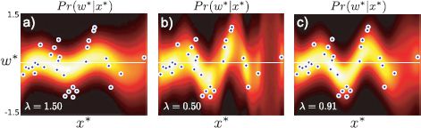
Figure 8.9 Gaussian process regression using an RBF kernel. a) When the length scale parameter λ is large, the function is too smooth. b) For small values of the length parameter the model does not successfully interpolate between the examples. c) The regression using the maximum likelihood length scale parameter is neither too smooth nor disjointed.
where the notation K[X,X] represents a matrix of dot products where element (i,j) is given by k[xi,xj].
Note that kernel functions may also contain parameters. For example, the RBF kernel (Equation 8.28) takes the parameter λ, which determines the width of the underlying RBF functions and hence the smoothness of the function (Figure 8.9). Kernel parameters such as λ can be learned by maximizing the marginal likelihood
This typically requires a nonlinear optimization procedure.
8.6 Sparse linear regression
We now turn our attention to the third potential disadvantage of linear regression. It is often the case that only a small subset of the dimensions of x are useful for predicting w. However, without modification, the linear regression algorithm will assign nonzero values to the gradient ![]() in these directions. The goal of sparse linear regression is to adapt the algorithm to find a gradient vector
in these directions. The goal of sparse linear regression is to adapt the algorithm to find a gradient vector ![]() where most of the entries are zero. The resulting classifier will be faster, since we no longer even have to make all of the measurements. Furthermore, simpler models are preferable to complex ones; they capture the main trends in the data without overfitting to peculiarities of the training set and generalize better to new test examples.
where most of the entries are zero. The resulting classifier will be faster, since we no longer even have to make all of the measurements. Furthermore, simpler models are preferable to complex ones; they capture the main trends in the data without overfitting to peculiarities of the training set and generalize better to new test examples.
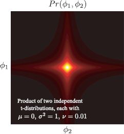
Figure 8.10 A product of two 1D t-distributions where each has small degrees of freedom v. This 2D distribution favors sparseness (where one or both variables are close to zero). In higher dimensions, the product of t-distributions encourages solutions where most variables are set to zero. Note that the product of 1D distributions is not the same as a multivariate t-distribution with a spherical covariance matrix, which looks like a multivariate normal distribution but with longer tails.
To encourage sparse solutions, we impose a penalty for every nonzero weighted dimension. We replace the normal prior over the gradient parameters ![]() = [
= [![]() 1,
1,![]() 2,…,
2,…,![]() D]T with a product of one-dimensional t-distributions so that
D]T with a product of one-dimensional t-distributions so that
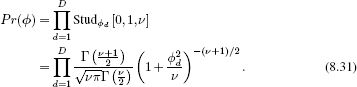
The product of univariate t-distributions has ridges of high probability along the coordinate axes, which encourages sparseness (see Figure 8.10). We expect the final solution to be a trade-off between fitting the training data accurately and the sparseness of ![]() (and hence the number of training data dimensions that contribute to the solution).
(and hence the number of training data dimensions that contribute to the solution).
Adopting the Bayesian approach, our aim is to compute the posterior distribution Pr(![]() |X, w,σ2) over the possible values of the gradient variable
|X, w,σ2) over the possible values of the gradient variable ![]() using this new prior so that
using this new prior so that
![]()
Unfortunately, there is no simple closed form expression for the posterior on the left-hand side. The prior is no longer normal, and the conjugacy relationship is lost.
To make progress, we reexpress each t-distribution as an infinite weighted sum of normal distributions where a hidden variable hd determines the variance (Section 7.5), so that
where the matrix H contains the hidden variables {hd}Dd=1 on its diagonal and zeros elsewhere. We now write out the expression for the marginal likelihood (likelihood after integrating over the gradient parameters ![]() ) as
) as
where the integral over Φ was computed using the same technique as used in Equation 8.12.
Unfortunately, we still cannot compute the remaining integral in closed form, so we instead take the approach of maximizing over hidden variables to give an approximate expression for the marginal likelihood
As long as the true distribution over the hidden variables is concentrated tightly around the mode, this will be a reasonable approximation. When hd takes a large value, the prior has a small variance (1/hd), and the associated coefficient ![]() d will be forced to be close to zero: in effect, this means that the dth dimension of x does not contribute to the solution and can be dropped from the equations.
d will be forced to be close to zero: in effect, this means that the dth dimension of x does not contribute to the solution and can be dropped from the equations.
The general approach to fitting the model is now clear. There are two unknown quantities – the variance σ2 and the hidden variables h and we alternately update each to maximize the log marginal likelihood.1
• To update the hidden variables, we take the derivative of the log of this expression with respect to H, equate the result to zero, and rearrange to get the iteration
![]()
where μd is the dth element of the mean μ of the posterior distribution over the weights ![]() and Σdd is the dth element of the diagonal of the covariance Σ of the posterior distribution over the weights (Equation 8.10) so that
and Σdd is the dth element of the diagonal of the covariance Σ of the posterior distribution over the weights (Equation 8.10) so that
![]()
and A is defined as
![]()
• To update the variance, we take the derivative of the log of this expression with respect to σ2, equate the result to zero, and simplify to get
![]()
Between each of these updates, the posterior mean μ and variance Σ should be recalculated.
In practice, we choose a very small value for the degrees of freedom (ν <10−3) to encourage sparseness. We may also restrict the maximum possible values of the hidden variables hi to ensure numerical stability.
At the end of the training, all dimensions of ![]() where the hidden variable hd is large (say > 1000) are discarded. Figure 8.11 shows an example fit to some two-dimensional data. The sparse solution depends only on one of the two possible directions and so is twice as efficient.
where the hidden variable hd is large (say > 1000) are discarded. Figure 8.11 shows an example fit to some two-dimensional data. The sparse solution depends only on one of the two possible directions and so is twice as efficient.
In principle, a nonlinear version of this algorithm can be generated by transforming the input data x to create the vector z = f[x]. However, if the transformed data z is very high-dimensional, we will need correspondingly more hidden variables hd to cope with these dimensions. Obviously, this idea will not transfer to kernel functions where the dimensionality of the transformed data could be infinite.
To resolve this problem, we will develop the relevance vector machine. This model also imposes sparsity, but it does so in a way that makes the final prediction depend only on a sparse subset of the training data, rather than a sparse subset of the observed dimensions. Before we can investigate this model, we must develop a version of linear regression where there is one parameter per data example rather than one per observed dimension. This model is known as dual linear regression.
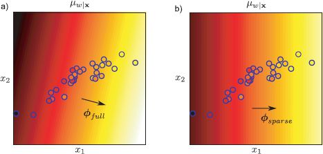
Figure 8.11 Sparse linear regression. a) Bayesian linear regression from two-dimensional data. The background color represents the mean μw|x of the Gaussian prediction Pr(w|x) for w. The variance of Pr(w|x) is not shown. The color of the datapoints indicates the training value w, so for a perfect regression fit this should match exactly the surrounding color. Here the elements of ![]() take arbitrary values and so the gradient of the function points in an arbitrary direction. b) Sparse linear regression. Here, the elements of
take arbitrary values and so the gradient of the function points in an arbitrary direction. b) Sparse linear regression. Here, the elements of ![]() are encouraged to be zero where they are not necessary to explain the data. The algorithm has found a good fit where the second element of
are encouraged to be zero where they are not necessary to explain the data. The algorithm has found a good fit where the second element of ![]() is zero and so there is no dependence on the vertical axis.
is zero and so there is no dependence on the vertical axis.
8.7 Dual linear regression
In the standard linear regression model the parameter vector ![]() contains D entries corresponding to each of the D dimensions of the (possibly transformed) input data. In the dual formulation, we reparameterize the model in terms of a vector ψ which has I entries where I is the number of training examples. This is more efficient in situations where we are training a model where the input data are high-dimensional, but the number of examples is small (I < D), and leads to other interesting models such as relevance vector regression.
contains D entries corresponding to each of the D dimensions of the (possibly transformed) input data. In the dual formulation, we reparameterize the model in terms of a vector ψ which has I entries where I is the number of training examples. This is more efficient in situations where we are training a model where the input data are high-dimensional, but the number of examples is small (I < D), and leads to other interesting models such as relevance vector regression.
8.7.1 Dual model
In the dual model, we retain the original linear dependence of the prediction w on the input data x so that
![]()
However, we now represent the slope parameters ![]() as a weighted sum of the observed data points so that
as a weighted sum of the observed data points so that
![]()
where ψ is a I × 1 vector representing the weights (Figure 8.12). We term this the dual parameterization. Notice that, if there are fewer data examples than data dimensions, then there will be fewer unknowns in this model than in the standard formulation of linear regression and hence learning and inference will be more efficient. Note that the term dual is heavily overloaded in computer science, and the reader should be careful not to confuse this use with its other meanings.
If the data dimensionality D is less than the number of examples I, then we can find parameters ψ to represent any gradient vector ![]() . However, if D > I (often true in vision where measurements can be high-dimensional), then the vector Xψ can only span a subspace of the possible gradient vectors. However, this is not a problem: if there was no variation in the data X in a given direction in space, then the gradient along that axis should be zero anyway since we have no information about how the world state w varies in this direction.
. However, if D > I (often true in vision where measurements can be high-dimensional), then the vector Xψ can only span a subspace of the possible gradient vectors. However, this is not a problem: if there was no variation in the data X in a given direction in space, then the gradient along that axis should be zero anyway since we have no information about how the world state w varies in this direction.
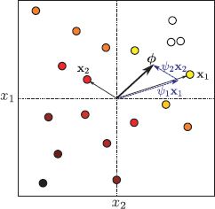
Figure 8.12 Dual variables. Two-dimensional training data {xi}Ii=1 and associated world state {wi}Ii=1 (indicated by marker color). The linear regression parameter ![]() determines the direction in this 2D space in which w changes most quickly. We can alternately represent the gradient direction as a weighted sum of data examples. Here we show the case
determines the direction in this 2D space in which w changes most quickly. We can alternately represent the gradient direction as a weighted sum of data examples. Here we show the case ![]() = ψ1x1 + ψ2x2. In practical problems, the data dimensionality D is greater than the number of examples I so we take a weighted sum
= ψ1x1 + ψ2x2. In practical problems, the data dimensionality D is greater than the number of examples I so we take a weighted sum ![]() = Xψ of all the datapoints. This is the dual parameterization.
= Xψ of all the datapoints. This is the dual parameterization.
Making the substitution from Equation 8.41, the regression model becomes
![]()
or writing all of the data likelihoods in one term
![]()
where the parameters of the model are θ = ψ,σ2}. We now consider how to learn this model using both the maximum likelihood and Bayesian approaches.
Maximum likelihood solution
We apply the maximum likelihood method to estimate the parameters ψ in the dual formulation. To this end, we maximize the logarithm of the likelihood (Equation 8.43) with respect to ψ and σ2 so that
![]()
To maximize this expression, we take derivatives with respect to ψ and σ2, equate the resulting expressions to zero, and solve to find
This solution is actually the same as for the original linear regression model (Equation 8.6). For example, if we substitute in the definition ![]() = Xψ,
= Xψ,
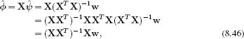
which was the original maximum likelihood solution for ![]() .
.
Bayesian solution
We now explore the Bayesian approach to the dual regression model. As before, we treat the dual parameters ψ as uncertain, assuming that the noise σ2 is known. Once again, we will estimate this separately using maximum likelihood.
The goal of the Bayesian approach is to compute the posterior distribution Pr(ψ|X,w) over possible values of the parameters ψ given the training data pairs {xi,wi}Ii=1. We start by defining a prior Pr(ψ) over the parameters. Since we have no particular prior knowledge, we choose a normal distribution with a large spherical covariance,
![]()
We use Bayes’ rule to compute the posterior distribution over the parameters
![]()
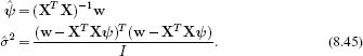
which can be shown to yield the closed form expression
![]()
where
![]()
To compute the predictive distribution Pr(w*|x*), we take an infinite weighted sum over the predictions of the model associated with each possible value of the parameters ψ,
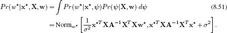
To generalize the model to the nonlinear case, we replace the training data X = [x1,x2,…,xI] with the transformed data Z =[z1,z2,…,zI] and the test data x* with the transformed test data z*. Since the resulting expression depends only on inner products of the form ZTZ and ZTz*, it is directly amenable to kernelization.
As for the original regression model, the variance parameter σ2 can be estimated by maximizing the log of the marginal likelihood which is given by
![]()
8.8 Relevance vector regression
Having developed the dual approach to linear regression, we are now in a position to develop a model that depends only sparsely on the training data. To this end, we impose a penalty for every nonzero weighted training example. We achieve this by replacing the normal prior over the dual parameters ψ with a product of one-dimensional t-distributions so that
![]()
This model is known as relevance vector regression.
This situation is exactly analogous to the sparse linear regression model (Section 8.6) except that now we are working with dual variables. As for the sparse model, it is not possible to marginalize over the variables ψ with the t-distributed prior. Our approach will again be to approximate the t-distributions by maximizing with respect to their hidden variables rather than marginalizing over them (Equation 8.35). By analogy with Section, 8.6 the marginal likelihood becomes
where the matrix H contains the hidden variables {hi}Ii=1 associated with the t-distribution on its diagonal and zeros elsewhere. Notice that this expression is similar to Equation 8.52 except that instead of every datapoint having the same prior variance σp2, they now have individual variances that are determined by the hidden variables that form the elements of the diagonal matrix H.
In relevance vector regression, we alternately (i) optimize the marginal likelihood with respect to the hidden variables and (ii) optimize the marginal likelihood with respect to the variance parameter σ2 using
![]()
and
![]()
In between each step we update the mean μ and variance Σ of the posterior distribution
![]()
where A is defined as
![]()
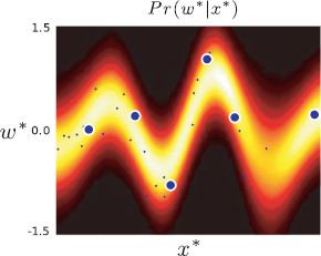
Figure 8.13 Relevance vector regression. A prior applying sparseness is applied to the dual parameters. This means that the final classifier only depends on a subset of the datapoints (indicated by the six larger points). The resulting regression function is considerably faster to evaluate and tends to be simpler: this means it is less likely to overfit to random statistical fluctuations in the training data and generalizes better to new data.
At the end of the training, all data examples where the hidden variable hi is large (say > 1000) are discarded as here the coefficients ψi will be very small and contribute almost nothing to the solution.
Since this algorithm depends only on inner products, a nonlinear version of this algorithm can be generated by replacing the inner products with a kernel function k[xi,xj]. If the kernel itself contains parameters, these may be also be manipulated to improve the log marginal variance during the fitting procedure. Figure 8.13 shows an example fit using the RBF kernel. The final solution now only depends on six datapoints but nonetheless still captures the important aspects of the data.
8.9 Regression to multivariate data
Throughout this chapter we have discussed predicting a scalar value wi from multivariate data xi. In real-world situations such as the pose regression problem, the world states wi are multivariate. It is trivial to extend the models in this chapter: we simply construct a separate regressor for each dimension. The exception to this rule is the relevance vector machine: here we might want to ensure that the sparse structure is common for each of these models, so the efficiency gains are retained. To this end, we modify the model so that a single set of hidden variables is shared across the model for each world state dimension.
8.10 Applications
Regression methods are used less frequently in vision than classification, but nonetheless there are many useful applications. The majority of these involve estimating the position or pose of objects, since the unknowns in such problems are naturally treated as continuous.
8.10.1 Human body pose estimation
Agarwal and Triggs (2006) developed a system based on the relevance vector machine to predict body pose w from silhouette data x. To encode the silhouette, they computed a 60-dimensional shape context feature (Section 13.3.5) at each of 400-500 points on the boundary of the object. To reduce the date dimensionality, they computed the similarity of each shape context feature to each of 100 different prototypes. Finally, they formed a 100-dimensional histogram containing the aggregated 100-dimemensional similarities for all of the boundary points. This histogram was used vector x. The body pose was encoded by the 3 joint angles of each of the 18 major body joints and the overall azimuth (compass heding) of the body. The resulting 55-dimensional vector was used as the world state w.
A relevance vector machine was trained using 2636 data vectors xi extracted from silhouettes that were rendered using the commercial program POSER from known motion capture data wi. Using a radial basis function kernel, the relevance vector machine based its solution on just 6% of these training examples. The body pose angles of test data could be predicted to within an average of 6° error (Figure 8.14). They also demonstrated that the system worked reasonably well on silhouettes from real images (Figure 8.1).
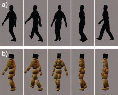
Figure 8.14 Body pose estimation results. a) Silhouettes of walking avatar. b) Estimated body pose based on silhouette using a relevance vector machine. The RVM used radial basis functions and constructed its final solution from just 156 of 2636 (6%) of the training examples. It produced a mean test error of 6.0° averaged over the three joint angles for the 18 main body parts and the overall compass direction of the model. Adapted from Agarwal and Triggs (2006).
Silhouette information is by its nature ambiguous: it is very hard to tell which leg is in front of the other based on a single silhouette. Agarwal and Triggs (2006) partially circumvented this system by tracking the body pose withrough a video sequence. Essentially, the ambiguity at a given frame is resolved by encouraging the estimated pose in adjacent frames in the sequence to be similar: information from frames where the pose vector is well defined is propagated through the sequence to resolve ambiguities in other parts (see Chapter 19).
However, the ambiguity of silhouette data is an argument for not using this type of classifier: the regression models in this chapter are designed to give a unimodal normal output. To effectively classify single frames of data, we should use a regression method that produces a multimodal prediction that can effectively describe the ambiguity.
8.10.2 Displacement experts
Regression models are also used to form displacement experts in tracking applications. The goal is to take a region of the image x and return a set of numbers w that indicate the change in position of an object relative to the window. The world state w might simply contain the horizontal and vertical translation vectors or might contain parameters of a more complex 2D transformation (see Chapter 15). For simplicity, we will describe the former situation.
Figure 8.15 Tracking using displacement experts. The goal of the system is to predict a displacement vector indicating the motion of the object based on the pixel data at its last known position. a) The system is trained by perturbing the bounding box around the object to simulate the motion of the object. b) The system successfully tracks a face, even in the presence c) of partial occlusions. d) If the system is trained using gradient vectors rather than raw pixel values, it is also quite robust to changes in illumination. Adapted from Adapted from Williams et al. (2005).©2005 IEEE.
Training data are extracted as follows. A bounding box around the object of interest (car, face, etc.) is identified in a number of frames. For each of these frames, the bounding box is perturbed by a predetermined set of translation vectors, to simulate the object moving in the opposite direction (Figure 8.15). In this way, we associate a translation vector wi with each perturbation. The data from the perturbed bounding box are extracted and resized to a standard shape, and histogram equalized (Section 13.1.2) to induce a degree of invariance to illumination changes. The resulting values are then concatenated to form the data vector xi.
Williams et al. (2005) describe a system of this kind in which the elements of w were learned by a set of independent relevance vector machines. They initialize the position of the object using a standard object detector (see Chapter 9). In the subsequent frame, they compute a prediction for the displacement vector w using the relevance vector machines on the data x from the original position. This prediction is combined in a Kalman filter-like system (Chapter 19) that imposes prior knowledge about the continuity of the motion to create a robust method for tracking known objects in scenes. Figures 8.15b–d show a series of tracking results from this system.
Discussion
The goal of this chapter was to introduce discriminative approaches to regression. These have niche applications in vision related to predicting the pose and position of objects. However, the main reason for studying these models is that the concepts involved (sparsity, dual variables, kernelization) are all important for discriminative classification methods. These are very widely used but are rather more complex and are discussed in the following chapter.
Notes
Regression methods: Rasmussen and Williams (2006) is a comprehensive resource on Gaussian processes. The relevance vector machine was first introduced by Tipping (2001). Several innovations within the vision community have extended these models. Williams et al. (2006) presented a semisupervised method for Gaussian process regression in which the world state w is only known for a subset of examples. Ranganathan and Yang (2008) presented an efficient algorithm for online learning of Gaussian processes when the kernel matrix is sparse. Thayananthan et al. (2006) developed a multivariate version of the relevance vector machine.
Applications: Applications of regression in vision include head pose estimation (Williams et al. 2006; Ranganathan and Yang 2008; Rae and Ritter 1998), body tracking (Williams et al. 2006; Agarwal and Triggs 2006; Thayananthan et al. 2006), eye tracking (Williams et al. 2006), and tracking of other objects (Williams et al; 2005; Ranganathan and Yang 2008).
Multimodal posterior: One of the drawbacks of using the methods in this chapter is that they always produce a unimodal normally distributed posterior. For some problems (e.g., body pose estimation), the posterior probability over the world state may be genuinely multimodal – there is more than one interpretation of the data. One approach to this is to build many regressors that relate small parts of the world state to the data (Thayananthan et al. 2006). Alternatively, it is possible to use generative regression methods in which either the joint density is modeled directly (Navaratnam et al. 2007) or the likelihood and prior are modeled separately (Urtasun et al. 2006). In these methods, the posterior compute distribution over the world is multimodal. However, the cost of this is that it is intractable to compute the posterior exactly, and so we must rely on optimization techniques to find its modes.
Problems
8.1 Consider a regression problem where the world state w is known to be positive. To cope with this, we could construct a regression model in which the world state is modeled as a gamma distribution. We could constrain both parameters α,β of the gamma distribution to be the same so that α = β and make them a function of the data x. Describe a maximum likelihood approach to fitting this model.
8.2 Consider a robust regression problem based on the t-distribution rather than the normal distribution. Define this model precisely in mathematical terms and sketch out a maximum likelihood approach to fitting the parameters.
8.3 Prove that the maximum likelihood solution for the gradient in the linear regression model is
![]()
8.4 For the Bayesian linear regression model (Section 8.2), show that the posterior distribution over the parameters ![]() is given by
is given by
![]()
where
![]()
8.5 For the Bayesian linear regression model (Section 8.2), show that the predictive distribution for a new data example x* is given by
![]()
8.6 Use the matrix inversion lemma (Appendix C.8.4) to show that
![]()
8.7 Compute the derivative of the marginal likelihood
![]()
with respect to the variance parameter σ2.
8.8 Compute a closed form expression for the approximated t-distribution used to impose sparseness.
![]()
Plot this function for ν = 2. Plot the 2D function [h1,h2] = q(h1)q(h2) for ν = 2.
8.9 Describe maximum likelihood learning and inference algorithms for a nonlinear regression model based on polynomials where
![]()
8.10 I wish to learn a linear regression model in which I predict the world w from I examples of D × 1 data x using the maximum likelihood method. If I > D, is it more efficient to use the dual parameterization or the original linear regression model?
8.11 Show that the maximum likelihood estimate for the parameters ψ in the dual linear regression model (Section 8.7) is given by
![]()
___________________________________
1More details about how these (nonobvious) update equations were generated can be found in Tipping (2001) and section 3.5 of Bishop (2006).
All materials on the site are licensed Creative Commons Attribution-Sharealike 3.0 Unported CC BY-SA 3.0 & GNU Free Documentation License (GFDL)
If you are the copyright holder of any material contained on our site and intend to remove it, please contact our site administrator for approval.
© 2016-2026 All site design rights belong to S.Y.A.