Make: AVR Programming (2014)

Part I. The Basics

Chapter 7. Analog-to-Digital Conversion I

Light Sensors and Slowscope

If there’s one thing I like about microcontrollers, it’s connecting the real world with the code world. And a lot of the real world is analog: voltages, currents, light levels, forces, etc., all take on continuously variable values. Deep inside the AVR, on the other hand, everything is binary: on or off. Going from the analog world to the digital is the job of the analog-to-digital converter (ADC) hardware. Using the built-in ADC, we’ll see how to use the AVR to take (voltage) readings from analog sensors and turn them into numbers that we can use inside our code.

Imagine that you’re building a robot or an interactive art piece. You might be interested in measuring temperature, distance to the nearest object, force and acceleration, sound pressure level, brightness, magnetic force, or other physical characteristics. The first step is to convert all of these physical quantities into a voltage using a specifically designed sensor of some sort. Then, you might have to modify this voltage input so that it’s in a range that’s usable by the AVR. Finally, the voltage is connected up to an AVR pin, and the internal ADC hardware converts the continuous voltage value into a number that you can use in your code like any other.

In this chapter, we’ll use the ADC and a serial connection to make a slow “oscilloscope.” We’ll interface with a light sensor, making a simple LED-display light meter. Finally, we’ll add in a potentiometer to create an adjustable-threshold night-light that turns a bunch of LEDs on when it gets dark enough. How dark? You get to decide by turning a knob!

WHAT YOU NEED

In this chapter, in addition to the basic kit, you will need:

§ Two light-dependent resistors (LDR) and a few resistors in the 10k ohm range to create a voltage divider.

§ A potentiometer—anything above 1k ohm will work.

§ LEDs hooked up to PORTB as always.

§ A USB-Serial adapter.

Analog sensors and electronics are by themselves huge topics, so I won’t be able to cover everything, but I’ll try to point out further interesting opportunities in passing. In this chapter, I’ll focus on simply using the AVR’s ADC hardware—taking continuous readings through clever use of interrupt service routines, and using the multiplexer so that you can read analog voltages from more than one source. Topics like input voltage scaling and oversampling and noise smoothing will have to wait for Chapter 12.

SENSORS

With the exception of a battery-charge monitor or something similar, you’re almost never interested in measuring a voltage directly. But because measuring voltages is so darn easy, you’ll find that many, many analog sensors convert whichever physical quantities they’re designed to measure (light, noise, or temperature) into a voltage. And once you’ve got a properly scaled voltage, you’re all set to read the value in through the ADC.

Designing sensors to put out carefully calibrated voltages in response to the physical world is both a science and an art in itself. When you don’t need absolute accuracy, though, there are a lot of interesting physical effects that end up in a voltage signal. For you as the microcontroller designer, browsing around through the world of different sensing possibilities can be inspirational.

One good source of cheap-and-easy ideas for sensors is Forrest Mims’ Electronic Sensor Circuits & Projects from the “Engineer’s Mini Notebook” series (Master Publishing, Inc., 2004).

ADC Hardware Overview

The onboard ADC peripheral is an incredibly complex system. Have a look at the block diagram in the datasheet to see for yourself. You might be tempted to just treat it all as a black-box, and I’m sure a lot of people do. But a quick look behind the curtain will help make sense of all the configuration options and the few tricky bits that it pays to be aware of. Figure 7-1 lays out all the major components of the ADC peripheral.

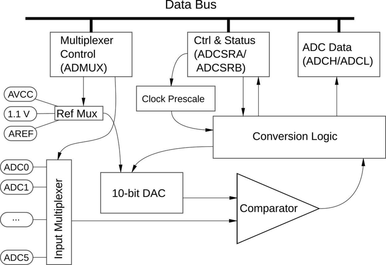
Figure 7-1. ADC hardware

At the heart of the ADC is actually a DAC—a digital-to-analog converter—and a comparator. The DAC generates a voltage that corresponds to a digital value that it takes as input. The comparator is a digital device that outputs a binary high or low value if the input signal coming from one of the ADC pins is higher or lower than the output of the DAC. Like playing a game of “20 Questions,” the conversion logic sets a voltage level on the DAC and then reads the value off the comparator to figure out if the input voltage is higher or lower than this DAC voltage. The ADC repeats this until it has located the input voltage between two of the 10-bit voltage levels that it can produce with the DAC.

The ADC has a number of options for the reference voltage it applies to the internal DAC, which enable you to tailor the voltage range over which the 10 bits are spread so that you get maximum resolution in end use. The ADC also has a number of triggering options. You can start an ADC conversion from your code, or any of the internal timer compare or overflow conditions, the external INT0 pin, or even the ADC itself—resulting in the so-called free-running mode where it’s continually sampling.

The ADC module can’t run at the full CPU clock speed, though, so it needs its own clock source. The good news is that it’s equipped with a clock prescaler (like the timers are) that can subdivide the CPU clock down to a usable speed. The bad news is that because you can change the CPU clock speed, it’s also your responsibility to figure out an appropriate prescaler for the ADC clock.

Because of all this complexity, the ADC module is a large chunk of silicon. It would be a shame to have only one ADC on board, though, and only be able to sample one sensor. As a compromise, the AVR (and most other microprocessors) shares the ADC module out over a number of pins. In our case, pins PC0 to PC5 are all available for use as ADC inputs (plus a couple more if you’re using the surface-mount version of the chips), with the catch that you can only take readings from one at a time, and you must switch between them. A multiway switch like this is called a multiplexer, or “mux” for short.

Finally, the ADC has to communicate with the rest of the chip through a bunch of hardware registers, both for configuration and for returning the digitized voltage value. So in summary, the ADC hardware is a beast. Heck, the ADC even draws power from its own separate power supply pin, AVCC!

HOW THE ADC WORKS: SUCCESSIVE APPROXIMATION

The AVR is a fundamentally digital chip, so how can it figure out the analog voltage on the input pin? Well, it can’t figure it out exactly, but it can figure out a range in which the analog value lies by asking a bunch of clever yes/no questions. The method the AVR’s ADC uses is called successive approximation.

Successive approximation works by taking a reference voltage (on the AREF pin) and dividing it in half using an internal 10-bit digital-to-analog converter. Then the input voltage is compared with this DAC voltage. If the input is higher, the ADC writes down a 1 and then sets the internal DAC at half the difference between AREF and AREF/2. If the input is lower, the ADC writes down a 0 and sets the DAC halfway between GND and AREF/2.

The ADC repeats these tests 10 times for a 10-bit result, changing the DAC level each time to cut the possible voltage range in half. If the most significant bit is a 1, then you know that input voltage is greater than AREF/2. If the most significant bits are (1,0), then you know that the voltage is greater than 1/2 AREF, but less than 3/4 AREF, etc. For each bit, the possible voltage range that the input can be in is cut in half, so that by the end of 10 bits, the ADC knows which of 1,024 bins the voltage is in, and the resulting 10-bit binary number points exactly at it.

As the AVR goes through this process of successive approximation, it needs to have a constant version of the input voltage. To do this, there’s a sample and hold circuit just on the frontend of the ADC that connects a capacitor to your voltage source and lets it charge up to the input voltage level. Then it disconnects the capacitor and the (now nearly constant) voltage on the capacitor is used in the successive approximation procedure. So even if the external voltage is changing rapidly, the ADC will have a snapshot of that voltage taken at the time that sampling started.

What does this mean for you, as chip-user and programmer? Using the ADC is going to boil down to first configuring an ADC clock speed (more on this later), and then instructing the ADC to start taking a sample by setting the “start conversion” bit in an ADC register. When the ADC is done, it writes this same bit back to zero. Between starting the ADC conversion and its finish, your code can either sit around and test for this flag, or set up an interrupt service routine to trigger when the ADC is done. Because the ADC is reasonably fast, I’ll often just use the (simpler) blocking-wait method. On the other hand, when you’re trying to squeeze out maximum speed from the CPU and ADC, the ISR method is the way to go. You’ll see examples of both here.

We’ll start with a minimum configuration and work our way up example by example to something more complex. To make full use of the ADC you can or must set:

§ The ADC clock prescaler (default: disabled, which means no conversions)

§ The voltage reference that defines the full scale (default: an externally supplied voltage)

§ The analog channel to sample from (default: external pin PC0)

§ An ADC trigger source (default: free-running if specified)

§ Interrupts to call when an ADC conversion is complete (default: none)

§ Other miscellaneous options including an 8-bit mode, turning off the digital input circuitry to save power, and more

Light Meter

Creating a simple light meter is a classic first ADC project. The sensor is cheap and simple to make, and there are a many different directions to extend the basic program just in software. Here, we’ll use the LEDs to display the amount of light hitting the sensor. If you calibrated this sensor, you could use it as an exposure meter for a camera. If you shine a light on the circuit from across the room with a laser bounced off a bunch of mirrors, you could make a beam-break detector suitable for securing your diamonds.

The Circuit

The sensor portion of this project is basically a voltage divider. A voltage divider is really just two resistors (or similar) in series between one voltage level and ground. Because the bottom end of the lower resistor is at ground, and the top end of the upper resistor at, say VCC, the middle point where they join together must be at some voltage in the middle. If the two resistances are equal, the voltage in the middle will be 1/2 VCC. If the top resistance is less than the bottom, the output voltage will be higher than 1/2, and vice versa.

To make our light sensor, we’re using an LDR for the top resistor and hooking up the middle-point output voltage to our ADC. So when the LDR is less resistive, we’ll read more voltage. The LDR gets less resistive when more light shines on it, so we’ll see a direct relationship between the light level and the voltage sent to the AVR—a simple light meter!

CADMIUM-SULFIDE LIGHT SENSOR

One of my favorite electronic components is the cadmium-sulfide, light-dependent resistor (LDR), also known simply as “photocells” or “photoresistors.” They’re cheap, relatively sturdy, and do just exactly what they are supposed to—provide a resistance that decreases as more and more light falls on them. Coupled with a fixed-value resistor, you get a voltage divider whose output depends on its illumination: a light-to-voltage converter.

LDRs are used everywhere: old-school camera light meters, streetlamp on/off circuits, automatic headlight sensors, beam-break detectors, and even sensors in telescopes. On the other hand, LDRs can be a little touchy to work with unless you know a few things:

§ LDRs vary a lot from one to the next in terms of their maximum resistance in the dark, so don’t expect any two to have exactly the same resistance in the same conditions. If you’ve got an ohmmeter, measure a few in the dark to see what I mean.

§ Lesser-known fact: LDRs also exhibit a temperature-dependent resistance.

§ You can burn an LDR out if you run too much current through it. And because the resistance drops as the light hitting it gets brighter, the fixed resistor can’t be too small: keep it above 200 ohms at 5 V.

§ If your sensor saturates in bright light, try decreasing the fixed resistor in the voltage divider. If you need more dark sensitivity, increase the fixed resistor.

§ LDRs are slow relative to microcontrollers, but faster than the human eye: they take between tens and hundreds of milliseconds to react to changes in light. My example LDR circuit is fast enough to detect the flicker in incandescent light bulbs that results from alternating current.

§ LDRs are most sensitive to light in the red-green wavelength range, so they pair up beautifully with red LEDs or lasers. Some even see into the infrared. They’re a little weaker in the blue-purple range. Their response curve is actually a lot like the human eye’s.

So connect one end of the LDR to VCC and the other to the fixed resistor to ground, as shown in Figure 7-2. The joint between the LDR and fixed resistor is our voltage output—connect this to pin PC0 on the AVR.

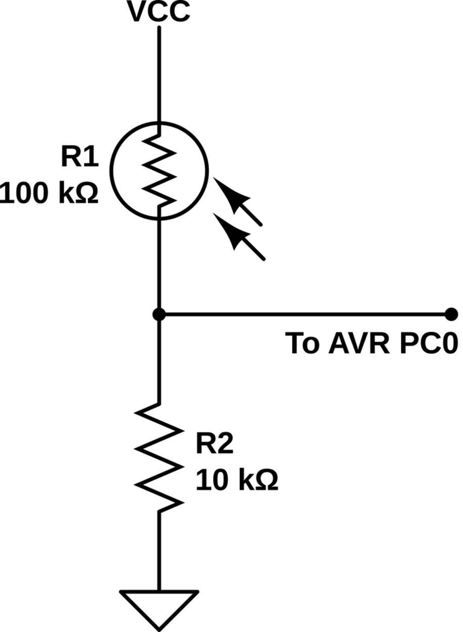
Figure 7-2. LDR voltage divider

A good rule of thumb for getting the maximum variability out of your LDR-based voltage divider is to use a fixed resistor that’s approximtely the square root of the LDR’s resistance at the brightest light level, multiplied by the resistance at the lowest light level:

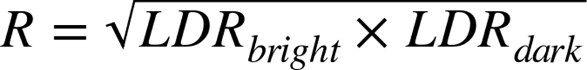
For instance, if the LDR measures 16k ohm in the light and 100k ohm when it’s dark, you’ll want roughly a 40k ohm resistor. For a sample of LDRs on my bench and indoor lighting conditions, the ideal resistor ended up in the 10k ohm to 100k ohm range, so measure and experiment in this range. (The value is also going to depend on how brightly lit your room is.) If you’ve got a 100k ohm potentiometer lying around, you can use that in place of the fixed resistor and you’ll have control over the sensitivity.

VOLTAGE DIVIDERS

You’ll start seeing voltage dividers everywhere once you know what to look for. Almost any time you have two passive components hooked together in series between two different voltage levels, and you’re reading out the value from the middle—you’ve got a voltage divider.

The basic voltage divider is just two resistors hooked end-to-end between the VCC and GND rails. We’re interested in the voltage in-between the two resistors, and this voltage is determined by the values of the two resistors. If both have the same resistance, the voltage taken from the midpoint is half of the input voltage. In general, you can get any voltage you’d like between GND and V_in by using the formula V_out = V_in × R₂ / (R₁ + R₂).

By analogy to water pressure in a piping system, where water pressure is like voltage, higher resistance corresponds to skinnier tubes. Smaller diameter piping restricts the flow of water, like higher resistance impedes the flow of electrons. If you pinch on a hose (increase the resistance), you’ll see more pressure upstream of the pinch and less downstream. In the same way, if you use a large resistor for R₂, more of the original V_in voltage (pressure) is present at the midpoint. If you decrease the resistance in R₂, the current flows through it relatively unimpeded, and the voltage/pressure at the junction is much lower.

To remember whether it’s R₁ or R₂ in the numerator, think about which resistor is dropping more of the voltage across it. One end of the pair of resistors is at 5 V, and the other end is at GND, 0 V. The total 5 V voltage difference from top to bottom must be split up between the two resistors. Because it takes more voltage to push a given current through a larger resistance, more of the voltage is dropped across the larger of the two resistors. If more voltage is dropped before we sample it, our V_out will be lower than half. If the larger resistor is on the bottom, most of the voltage drop occurs after we measure the voltage, so V_out will be greater than half.

Besides resistor-resistor voltage dividers, the resistor-capacitor lowpass filter we will use in Chapter 10 is another example of a voltage divider. Look at it again. We’re taking our output signal from between a resistor and capacitor that are connected in series to GND. Capacitors have a resistance to passing current that’s similar to resistors, except that it’s frequency-dependent. Capacitors block DC current entirely, but let higher and higher frequency AC current through with less and less resistance. (This resistance to AC current is called reactance, but you can think of reactance as a frequency-dependent resistance.) So if you look at the filter this way, you’ll see that the capacitor at the bottom of the circuit is more and more resistive as the frequency lowers, passing through more of the voltage at lower frequencies, and making a low-pass filter.

This circuit’s great on a breadboard, because it’s just two parts and a wire, or you can “sensorize” it by soldering the LDR and fixed resistor together and adding some wires. You can also increase the directionality of your sensor by wrapping the LDR in a bit of black electrical tape to make a snoot so that it is only sensitive to light falling on it from one direction. If you’re making a beam-break detector, this’ll also help protect the sensor from ambient light in the room, and make it more reliable. Figure 7-3 demonstrates the basic ideas.

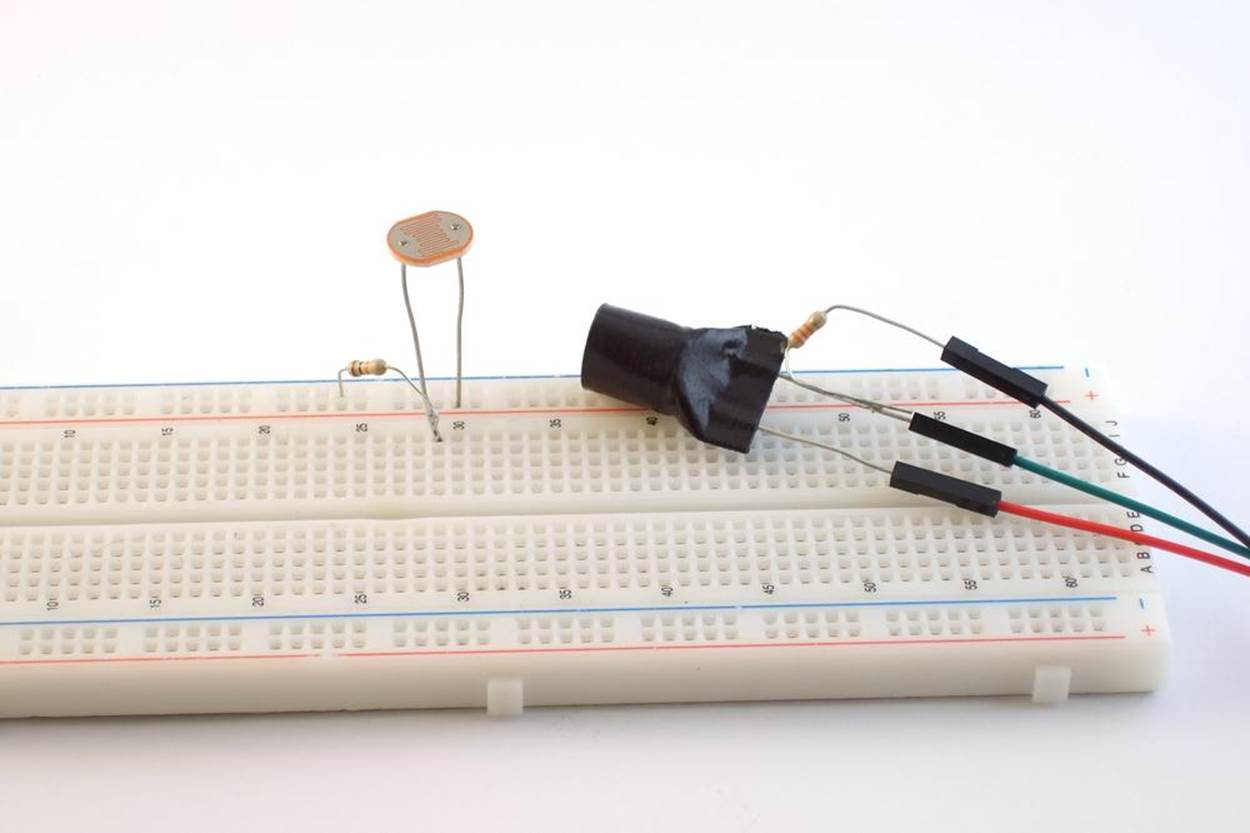
Figure 7-3. LDR sensors

ADC power pins

Aside from the sensor, there’s one tweak we’ll have to the AVR setup—powering up the ADC. There are two “special” pins connected to the ADC that are important for powering the hardware and for stabilizing the reference voltage. Good analog circuit design practice dictates that we use a separate source of 5 V for the chip (which has all sorts of quick switching and power spikes) and for the ADC, which needs a stable value to be accurate.

Ideally, you’d run a second wire directly from your 5 V source to the AVCC pin, rather than sharing the line that supplies the AVR with power. You should probably use this second, analog-only, 5 V rail to provide power to the light sensor as well. If you’re measuring very small voltage differences or high-frequency signals, this all becomes much more important, and you may need to use even more tricks to stabilize the AVCC.

Here, we’re not looking for millivolt accuracy, and we’re only sampling a few times per second. Feel free to get power to AVCC and the sensor however you’d like—just make sure you get 5 V to AVCC somehow. Without power, the ADC won’t run. I’ve made this mistake a bunch of times, and end up scratching my head about what’s wrong in my ADC init code for far longer than is productive.

If you’ve hooked up the AVCC and the LDR with a resistor, you should have something that looks like Figure 7-4. Of course, you’ll still have the programmer connections as well. You should also have the eight LEDs still hooked up to the B pins.

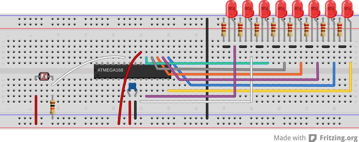
Figure 7-4. LDR voltage divider on the breadboard

LDR alternative: potentiometer

If you don’t happen to have an LDR handy, you really owe it to yourself to go out and get a few. Trust me on this. However, you can also “simulate” one so that you can experiment with the code and the setup here. The LDR and it’s resistor are simply making a variable voltage divider, so anything else along those lines will work as well. The obvious candidate is a potentiometer (pot). Any value of pot will do, as long as it’s greater than 1k ohm resistance.

Potentiometers are three-terminal devices. Essentially there’s a resistive track connecting the two outermost pins—that’s the rated (maximum) resistance. The middle pin is connected to a wiper that scans across the surface of the resistor as you turn the knob. The result is that when you turn the potentiometer knob one way, the resistance between the wiper and one outside pin increases while the resistance between the wiper and the other decreases.

Imagine that you’ve got a 10k ohm potentiometer with the knob turned exactly to the middle. The resistance from the wiper to either side will read 5k ohms, and if you put a voltage across the two outside pins, you’d find exactly half of that voltage on the wiper. Turn the knob one way, and the 10k ohms is split up, perhaps, 7k and 3k. If you apply 5 V across the outside pins, and the 3k resistance is on the GND side, the voltage at the wiper will be 5 V × 3 / (3 + 7) = 1.5 V.

To make a long story short, a potentiometer tied to the voltage rails makes a nice adjustable voltage for experimenting around with ADCs, and also a tremendously useful input device if you need a user to select from more than a couple of choices—just mark them out on a dial and read the ADC values in. Even if you do have an LDR lying around to play with, it’s probably worth your while to experiment some with potentiometers. An example circuit is shown in Figure 7-5.

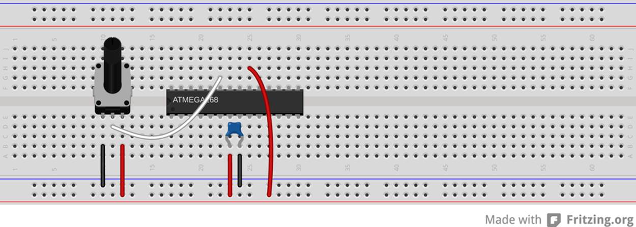
Figure 7-5. Potentiometer voltage divider on the breadboard

The Code

Because this is our first project with the ADC, we’ll necessarily have to talk a little bit of hardware initialization. First, let’s work through the event loop, as listed in Example 7-1, and then we’ll come back and clean up the details.

Example 7-1. lightSensor.c Listing

// Quick Demo of light sensor

// ------- Preamble -------- //

#include <avr/io.h>

#include <util/delay.h>

#include "pinDefines.h"

// -------- Functions --------- //

static inline void initADC0(void) {

ADMUX |= (1 << REFS0); /* reference voltage on AVCC */

ADCSRA |= (1 << ADPS1) | (1 << ADPS0); /* ADC clock prescaler /8 */

ADCSRA |= (1 << ADEN); /* enable ADC */

}

int main(void) {

// -------- Inits --------- //

uint8_t ledValue;

uint16_t adcValue;

uint8_t i;

initADC0();

LED_DDR = 0xff;

// ------ Event loop ------ //

while (1) {

ADCSRA |= (1 << ADSC); /* start ADC conversion */

loop_until_bit_is_clear(ADCSRA, ADSC); /* wait until done */

adcValue = ADC; /* read ADC in */

/* Have 10 bits, want 3 (eight LEDs after all) */

ledValue = (adcValue >> 7);

/* Light up all LEDs up to ledValue */

LED_PORT = 0;

for (i = 0; i <= ledValue; i++) {

LED_PORT |= (1 << i);

}

_delay_ms(50);

} /* End event loop */

return (0); /* This line is never reached */

}

The event loop starts off by directly triggering the start of a read from the ADC. Here, we first set the “ADC start conversion” (ADSC) bit in the “ADC Status Register A” to tell the ADC to sample voltage and convert it into binary for us. Because an ADC conversion doesn’t take place instantaneously, we’ll need to wait around for the result to become ready to use. In this example, I’m using a blocking-wait for the ADC; the loop_until_bit_is_clear() just spins the CPU’s wheels until the ADC signals that it’s done by resetting the ADSC bit.

If you’re reading up on the ADC in the datasheet, this mode of triggering is called “single-conversion mode” because our code initiates the conversion, and when it’s done, the ADC waits for further instructions. This is in contrast to “free-running mode,” in which the ADC retriggers itself as soon as it’s completed a conversion, or other triggering modes where you can assign the INT0 pin or even timer events to start an ADC conversion.

After a conversion is complete, the virtual register ADC contains a number from zero to 1,023 that represents the voltage (scaled by AREF) on the selected pin. I say “virtual” because the 10-bit ADC result is too large to fit in a normal 8-bit register, so it’s spread out over two registers: ADCL contains the least significant eight bits and ADCH contains the most significant two bits, and is padded with zeros. The compiler, GCC, lets us access these two registers as if they were a single 16-bit number.

Next, we want to send the value over the serial port to our computer. To make things easy, we convert the 10-bit number into a single 8-bit byte so that it’s easier to send over serial. A two-bit right-shift converts it down.

Finally, as eye-candy, the code displays the voltage/light level on our eight LEDs. Here’s a trick I end up using a lot when displaying data on a small number of LEDs. We have eight LEDs, or three-bits worth of them. We can use yet another bit shift to reduce our current eight-bit value down to three. (Or you can think if it as dividing a number between 0 and 255 by 32 so that it’s always between zero and eight.) Then to create a bargraph-like display, the code lights up each i‘th LED in a for loop up to the one that represents the scaled ADC value.

Besides the visualization on the LEDs, you can display the values on your computer. The Python routine serialScope.py provides rather nice feedback when debugging something like this, and it’s fun to watch the graph change as you wave your hand over the light sensor. When you’re done playing around with that, let’s look into the initialization.

ADC Initialization

Now let’s look in-depth at the ADC initialization in the initADC0() function. There are three principle registers that configure the ADC: ADMUX controls the multiplexer and voltage source; ADCSRA (status register A) controls the prescaler, enables the ADC, and starts conversions; and ADCSRB controls the triggering. And because we’ll be running in the so-called single conversion mode, we don’t need to worry about trigger sources. So have a look at the datasheet for the ADMUX and ADCSRA registers and follow along.

First, we set up the voltage reference for the chip. Because we’re using a light sensor that’s set up to output voltage in the same 0–5 V range as the chip is operating, we’ll set the reference voltage to AVCC. Because the AVR is internally connecting the AREF andAVCC pins together, we can add a decoupling capacitor between AREF and ground to further stabilize the analog reference voltage. It’s not necessary here, but it’s quick and easy if you’d like.

Next, we set up the ADC clock prescaler. Because we’re running the chip at 1 MHz off of the internal oscillator, and the ADC wants to run between 50 kHz and 200 kHz, we’ll pick a prescaler of 1/8, resulting in a 125 kHz sampling frequency. If you’re feeling brave, you can change this to 250 kHz, but the results aren’t guaranteed to work.

Providing the ADC with its own prescaled clock source is a pain if you’re running the AVR’s CPU clock at other frequencies, but at the end of the day, it’s just math. The ADC prescaler gives you the choice of dividing the CPU clock by 2, 4, 8, 16, 32, 64, or 128. Your goal is to pick one of these divisors that sets the ADC clock between 50 kHz and 200 kHz. Rather than go through this calculation every time, Table 7-1 provides a cheat sheet.

Table 7-1. ADC prescaler options

Note that I’ve included a couple of ADC clock frequencies that are just outside of the official 50–200 kHz range. Although I can’t figure why you’d want to run the ADC clock any slower than you have to, they seem to work. Maybe you save a little power?

On the fast end of things, the datasheet notes that running the ADC clock at speeds higher than 200 kHz is possible, with reduced resolution. I’ve included the clock settings for 250 kHz because I’ve found that it’s worked for me. You’re on your own here: Atmel only guarantees the ADC to run at 10-bits resolution up to 200 kHz, but I’ve never had trouble or noticed the lack of accuracy at 250 kHz.

Wrapping up the ADC initialization section, we’ll enable the ADC circuitry. This final step, enabling the ADC, is one of those small gotchas—do not forget to enable the ADC by setting the ADEN bit when you’re using the ADC!

So to recap the initialization: we’ve set the voltage reference. We’ve set the ADC clock prescaler. And finally, we’ve enabled the ADC. This is the simplest initialization routine that will work. What’s missing? We didn’t configure the multiplexer—but the default state is to sample from pin PC0, so we don’t need to. And we didn’t set up any triggering modes because we’re going to trigger the ADC conversions ourselves from code. So we’re set.

ADC GOTCHAS

So you’re not getting output from the ADC or it’s not changing? Here’s a quick troubleshooting checklist:

1. Did you hook up AVCC? The ADC needs power, and it needs to be within around 0.6 V of the AVR’s VCC.

2. Did you set a voltage reference with the REFSx bits in ADMUX? By default the AVR is looking for an external voltage reference on the AREF pin. If you’d like to use the AVCC as AREF, you have to set REFS0 in ADMUX.

3. Did you set the ADC prescaler? The ADC needs a clock source.

4. Did you set the ADEN bit to enable the ADC?

5. Do you have the correct channel selected in the multiplexer? Remember that they’re referenced by binary value rather than bit value.

6. Finally, if you’re reading the ADC values out independently, make sure that you read the low byte, ADCL, before you read the high byte, ADCH. For whatever reason, the ADCH bytes aren’t updated until ADCL is read in 10-bit mode. (I just avoid this snafu by reading ADC, and letting the compiler take care of the ordering for me.)

And if none of this is working, are you sure that your sensor is working? Try outputting the ADC data over the serial port and connecting the ADC pin to AREF and GND, respectively, to make sure that the problem lies in your code and not in a broken sensor. Or if you can, hook the sensor up to a voltmeter or oscilloscope. Is it behaving as you expect?

Extensions

OK, so now you’ve got a simple light meter. What can you do with it? First off, you could make a beam-break sensor. Aim a laser pointer or light of any kind at the light sensor and then walk through it. In your code, you can test if the value is greater or less than some threshold, and then light up LEDs or sound an alarm or something. Since you’re sending the data across to your computer, you could even tweet when someone breaks the beam.

Or you can send data (slowly!) from one AVR to another using light. Just remember that the LDR has about a 10–20 ms reaction time, which means bitrates like 50–100 baud. (You can get a lot faster with a photodiode, but that’s a different electrical setup.)

Or combine the AVR with some additional memory, and you can make a light-level logger. Put it out in your garden and record how many hours of what intensity sunlight your plants receive. Measure their growth along with it, and you’ve got the makings of some real plant science.

VACTROLS

A fantastic application for LDRs (totally unrelated to the one in this chapter, but I can’t resist) is providing microcontroller-controlled resistance for all sorts of circuits. Imagine that you had a circuit that relies on turning a potentiometer to create a variable resistance. (A perfect example is a guitar effect pedal, the kind that makes an electric guitar go waka-waka-wow-wow.) Wouldn’t it be nice if you could have your microcontroller turn the knob for you?

The trick is to tape an LDR face-to-face with an LED using black electrical tape so that the only light hitting the LDR comes from the LED. Now you’ve effectively got an LED-controlled resistor. The idea here is old—going back to the early 1900s—but a popular implementation of the circuit was trademarked in the 1960s as the “Vactrol” and the name stuck. In the analog-circuits days, Vactrols were used to turn varying currents into varying resistances, by brightening or dimming a light and thus lowering or raising the resistance of the LDR.

Now let’s digitize the Vactrol. In Chapter 10 you will see how you could pulse an LED quickly, using the duty cycle to make it appear to dim and brighten in a nearly continuous fashion. Taking advantage of the LDR’s relatively slow response time, you can PWM the LED, and thus digitally control the LDR’s resistance. Now you’ve got an 8-bit PWM-controlled resistor with a very wide range of resistances. Solder this into your guitar effects box, and your AVR chip can take care of the knob-twiddling for you.

The only limit to the PWM-Vactrol is that the LDR can’t handle much power, so if you’re substituting out a pot that moves significant current, you might want to consider hooking the LDR up to the base of a (power) transistor to supply the current. How to hook this up is application dependent, so if you’re going to do this, you’ll need to learn a thing or two about driving loads with transistors. I’ll cover this a little bit in Chapter 15, but otherwise I recommend a good book on introductory electronics. Practical Electronics for Inventors by Paul Scherz (McGraw-Hill) is a good one. The Art of Electronics by Horowitz and Hall (Cambridge University Press) is a little tougher read, but is an absolute classic.

Slowscope

In the light sensor example, we triggered an ADC conversion and then displayed the light reading on eight LEDs. You could also kind of visualize the light levels by watching the LEDs light up and turn off. But if you wanted to look at simple voltages with more resolution, or see some trace of them over time, you’ll want an oscilloscope. Old-school analog oscilloscopes would trace out a changing voltage over time by sweeping a light beam across a phosphorescent screen at a fixed speed, while the voltage applied to an input would deflect the beam up or down so that the end result was a display of the changing voltage levels over time. They’re tremendously useful if, like me, you like to visualize signals to “see” what’s going on.

When you’re debugging an ADC circuit, for instance, an oscilloscope can be particularly useful. But what if you don’t have one handy? Well, in this section you’ll set up the AVR’s ADC in free-running mode and transmit the digitized values back to your desktop computer. From there, you can either store it or plot it. To get a quick-and-dirty impression of what’s going on with the ADC voltage, you can simply plot the values out on the screen, making a sort of serial-port-speed limited, zero-to-five-volt oscilloscope—the “slowscope.” (Rhymes with “o-scope.”)

Because you’re already set up for measuring light levels as voltage using the LDR voltage divider, let’s use that for the demo. Plus, it’s nice to see what happens on your desktop computer’s screen as you wave your hands around over the light sensor.

For the circuit, all that’s left is to connect your USB-Serial converter to the AVR as you did in Chapter 5. In fact, all you’ll need is to connect the TX line from the AVR to the RX line on your USB-Serial converter.

The AVR Code

The AVR code in Example 7-2 is a quick exercise in configuring the ADC to work in free-running mode where it’s continually taking samples. Because there’s always a fresh ADC value ready to be read out, you can simply write it out to the serial port whenever you feel like it—in this case after a fixed time delay that determines the sweep speed of your scope.

Example 7-2. slowScope.c listing

// Slow-scope. A free-running AVR / ADC "oscilloscope"

// ------- Preamble -------- //

#include <avr/io.h>

#include <util/delay.h>

#include "pinDefines.h"

#include "USART.h"

#define SAMPLE_DELAY 20 /* ms, controls the scroll-speed of the scope */

// -------- Functions --------- //

static inline void initFreerunningADC(void) {

ADMUX |= (1 << REFS0); /* reference voltage on AVCC */

ADCSRA |= (1 << ADPS1) | (1 << ADPS0); /* ADC clock prescaler /8 */

ADMUX |= (1 << ADLAR); /* left-adjust result, return only 8 bits */

ADCSRA |= (1 << ADEN); /* enable ADC */

ADCSRA |= (1 << ADATE); /* auto-trigger enable */

ADCSRA |= (1 << ADSC); /* start first conversion */

}

int main(void) {

// -------- Inits --------- //

initUSART();

initFreerunningADC();

// ------ Event loop ------ //

while (1) {

transmitByte(ADCH); /* transmit the high byte, left-adjusted */

_delay_ms(SAMPLE_DELAY);

} /* End event loop */

return (0); /* This line is never reached */

}

To get a feel for how little code is needed once you get all of AVR’s hardware peripherals configured, have a look down at the main() function’s event loop. All it does is delay for a few milliseconds so that your screen doesn’t get overrun, and then sends across the current ADC value. All of the interesting details, and there are at least two of them, are buried in the ADC initialization function. What’s different from the last example? Glad you asked!

The line:

ADMUX |= (1 << ADLAR); /* left-adjust result, return only 8 bits */

left-adjusts the ADC value. Because the ADC has a 10-bit resolution, there are two ways you can pack it into the two 8-bit ADC registers, ADCH and ADCL. If you’d like to use the entire 10-bit value, it’s convenient to leave the left-adjust bit in its default state. These two options are illustrated in Figure 7-6. When the ADLAR bit is zero, the top byte, ADCH, only contains the top two bits of the ADC result. This way, if you read both bytes into a 16-bit result, you get the right number.

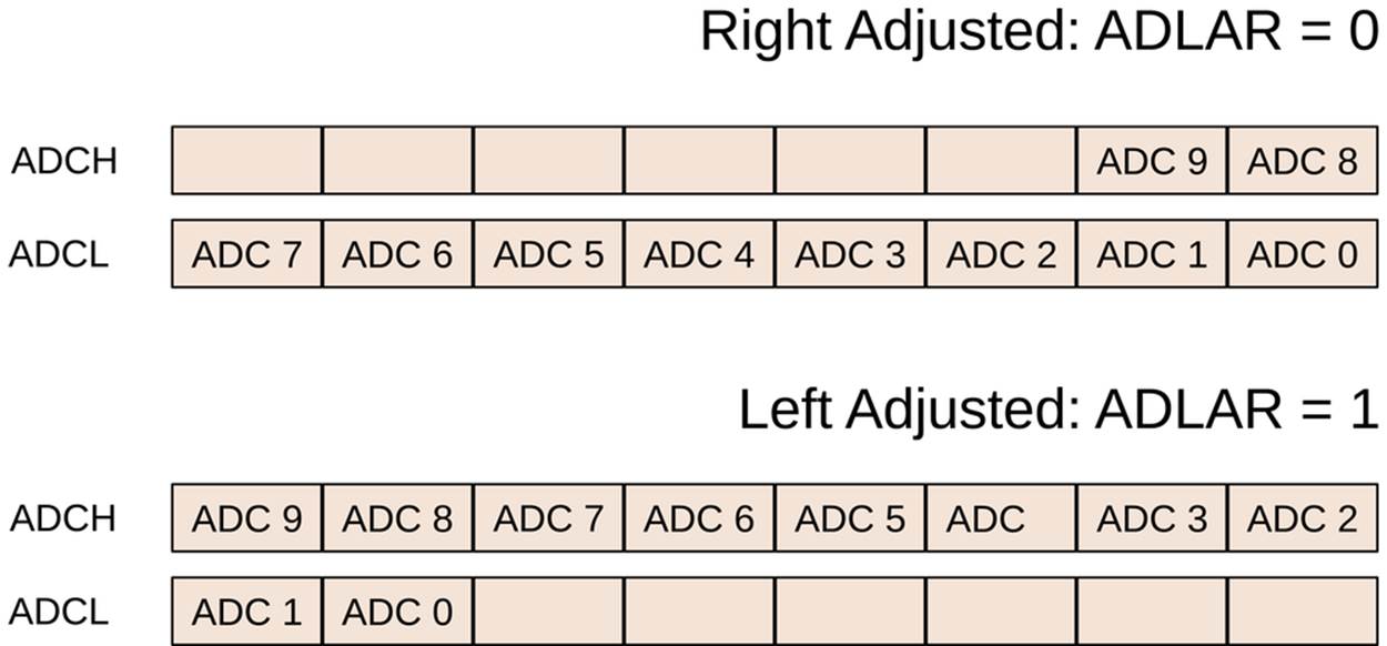
Figure 7-6. ADC result bit alignment

The alternative, which we use here, is to essentially throw away the least significant two bits by left-adjusting the top byte into ADCH and leaving the least significant two bits in ADCL. The AVR shifts the 10-bit byte over by six bits for you, so that the ADCH register contains a good 8-bit value. It’s an easy shortcut that saves you the bit-shifting when you only need 8-bit precision.

The other bit of interest in the ADC initialization routine concerns setting up and enabling free-running mode. All three lines of:

ADCSRA |= (1 << ADEN); /* enable ADC */

ADCSRA |= (1 << ADATE); /* auto-trigger enable */

ADCSRA |= (1 << ADSC); /* start first conversion */

are needed to make free-running mode work. The first sets the ADC auto-trigger enable bit, which turns on free-running mode. This sets up the ADC to start another sample as soon as the current sample is finished. You still have to start up the initial conversion, so I set the ADSC bit as I did in normal, one-shot mode to start up the first conversion. Then, because ADATE is set, the next conversion follows along automatically.

If you read the datasheet section on the ADC auto-trigger source, you’ll find that you can actually trigger conversions automatically a whole bunch of ways—when external pins changing logic state or from the AVRs internal timer/counter modules. But the default is to use the signal from the ADC’s own conversion-complete bit to trigger the next conversion, and that’s what we’re doing here. This means that as soon as the ADC finishes one reading, it will start up the next without any user intervention: “free-running.”

But you have to remember to kick it off initially at least that one time, hence the ADSC.

The Desktop Code

The AVR is sending data across the serial line to your desktop computer. All that’s left to do is plot it. I find this short bit of Python code in Example 7-3 so useful that I had to throw it in here. There’s all sorts of cosmetic and performance improvements you could make, but there’s a lot to be said for just printing the numbers out on the screen.

Example 7-3. serialScope.py listing

import serial

def readValue(serialPort):

return(ord(serialPort.read(1)))

def plotValue(value):

""" Displays the value on a scaled scrolling bargraph"""

leadingSpaces = " " * (value*(SCREEN_WIDTH-3) / 255)

print "%s%3i" % (leadingSpaces, value)

def cheapoScope(serialPort):

while(1):

newValue = readValue(serialPort)

plotValue(newValue)

if __name__ == "__main__":

PORT = '/dev/ttyUSB0'

BAUDRATE = 9600

TIMEOUT = None

SCREEN_WIDTH = 80

## Take command-line arguments to override defaults above

import sys

if len(sys.argv) == 3:

port = sys.argv[1]

baudrate = int(sys.argv[2])

else: # nothing passed, use defaults

print ("Optional arguments port, baudrate set to defaults.")

port, baudrate = (PORT, BAUDRATE)

serialPort = serial.Serial(port, baudrate, timeout=TIMEOUT)

serialPort.flush()

cheapoScope(serialPort)

The code makes heavy use of the Python pyserial library. If you don’t already have this installed, go do so now! See Installing Python and the Serial Library for installation instructions.

The three functions that make the scope work include readValue() that gets a single byte from the serial stream and converts it into an ordinal number. This way when the AVR sends 123, the code interprets it as the number 123 rather than {, which is ASCII character number 123.

Next plotValue() takes the value and prints an appropriate number of leading spaces, and then the number, padding to three digits with empty space. Finally, cheapoScope() just wraps an infinite loop around these two other functions. A new value is read in, then plotted. This goes on forever or until you close the window or press Ctrl-C to stop it.

If you call serialScope.py from the command line, it allows you to override the default serial port and baud rate configurations. On the other hand, once you know how your serial port is configured, you might as well hardcode it in here by editing the PORT andBAUDRATE definitions.

While looking through the defaults, if you’d like the program to quit after a few seconds with no incoming data, you can reset TIMEOUT to a number (in seconds). If you have a particularly wide or skinny terminal window, you can also change SCREEN_WIDTH.

The only little trick here is that before running the scope, the code flushes the serial port input buffer. Depending on your operating system, it may be collecting a bunch of past values from the serial port for you. This is normally a good idea, but here we’d like to start off with a clean slate so that we instantly read in the new values from the AVR. Hence, we flush out the serial buffer before calling cheapoScope() and looping forever.

Synergies

This sort of simple desktop computer scripting can greatly expand on the capabilities and debugging friendliness of the AVR environment. You saw in Chapter 5 how you can expand the AVR’s capabilities dramatically by taking in information from your desktop computer. Here, we’re doing the opposite.

If you’re adept with Python, I encourage you to make a fancier scope display if you’d like. The Python code could also easily be expanded out to a general-purpose data logger application if you’d like. Just open a file on your hard disk and start writing the values to it. Import the datetime module and timestamp them. Heck, import the csv module and you can import the data straight into a spreadsheet or statistics package. Even with such simple tools, if you combine them right, the world is your oyster.

Debugging the ADC is sometimes tricky. You won’t always know a priori what types of values to expect. Writing code to detect a shadow is much easier when you know just exactly how dark the shadow is, or how light it is in the room the rest of the time. Seeing how your signal data looks in real time helps your intuition a lot.

I hope you get as much use out of these simple “oscilloscope” routines as I do. Or at least that you have a good time waving your hand over the light sensor for a little bit. I’m pretty sure I can tell which direction I’m moving my hand—the thumb and pinkie fingers cast different shadows. Who knew? I wonder if I can teach the AVR to detect that?

AVR Night Light and the Multiplexer

We just saw how to use single ADC conversions, and then ADC conversions in free-running mode. What’s next? Learning how to use more than one of the ADC channels “at once”! We’ll stick with our light sensor on ADC0 / PC0 and add in a potentiometer on ADC3 / PC3. Switching between the two rapidly and comparing their voltage values in software will give us an easily adjustable night light that turns on at precisely the level of darkness that we desire.

OK, I’ll admit it’s not that cool a project, but it gives us a good excuse to learn about the ADC multiplexer and play around with reading values from potentiometers, both of which are fundamental uses of the ADC hardware.

Multiplexing

Because the internal ADC is a fairly complex bit of circuitry, it’s not too surprising that there’s only one of them per microcontroller. But what to do if you’d like to monitor several analog sensors or voltages? The approach that the AVR, and most other microcontrollers, take is to multiplex the ADC out to multiple pins; the single input to the ADC on the inside of the chip is connected through a six-way switch to external pins, enabling you to sample analog voltages on any one of the six PCn pins at a time.

If you’d like to sample from two or three different analog sources, you’ll need to switch between the pins, sampling each one at a time and then moving on to the next. And as always with the AVR’s hardware peripherals, this is done by telling an internal hardware register which channel you’d like to sample from.

This sounds obvious, but you also have to take care to be sure that you switch channels in the multiplexer before the start of an ADC sampling cycle. This is only really a problem in “free-running” mode, in which the ADC samples continually. In free-running mode, when you change the multiplexer, the AVR doesn’t restart the sampling automatically. This means that the first sample after you’ve changed the multiplexer will still be from the old analog source—you need to wait at least one complete ADC cycle before getting a value from the new channel. In my experience, it’s a lot easier to trigger each sample yourself (through mainloop or interrupt), because it’s easier to verify that you’ve set up the multiplexer correctly without any complex bookkeeping.

Setting the Mux Bits

The multiplexer is a tiny bit tricky to program, so I hope you haven’t forgotten all you learned about bit twiddling from Chapter 4. The problem is the following: the low four bits control which ADC pin is used for input, but the upper three control the voltage reference and switch between 8-bit mode and 10-bit mode as we saw in the slowScope code. When you change the multiplexer channel in ADMUX, you want to change the bottom four bits without modifying the upper four. To see what I mean, look at Figure 7-7.

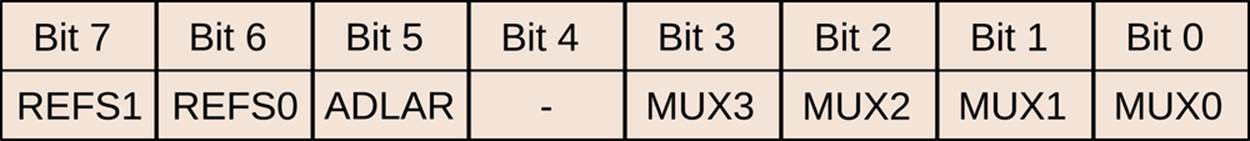
Figure 7-7. ADMUX register bits

To sample from ADC3, you set both the MUX0 and MUX1 bits and make sure that MUX2 and MUX3 are zeroed, because three in binary is 0011, right? But it’s lousy to have to think about setting each bit individually. Wouldn’t it be nicer to just write a three to the register? Sure, but then you’d end up clobbering the high bits. What if you just AND a three into the register? It doesn’t clear out the other low bits, if any were set. For instance, if you were sampling on channel five before with MUX2 and MUX1 set, you’d need to make sure that the MUX2 bit was cleared to get back to channel three.

The easiest solution is to first clear out the bottom four bits, and then AND in your desired channel number. This takes two conceptual steps. To change to ADC3 for instance, you first clear all the low bits and then write the number three back in:

ADMUX = ADMUX & 0b11110000; // clear all 4 mux bits

ADMUX = ADMUX | PC3; // set the bits we want

Notice that the top four bits aren’t changed by either of these instructions. You’ll often see this written with the clear and set steps combined into one line like this:

ADMUX = (0b11110000 & ADMUX) | PC3;

/* or, the ADC macro synonyms */

ADMUX = (0b11110000 & ADMUX) | ADC3;

/* or, in hex for the lazy typer */

ADMUX = (0xf0 & ADMUX) | ADC3;

/* or with numbers instead of macros */

ADMUX = (0xf0 & ADMUX) | 3;

This bitmask-style code is easily extensible when you need to loop over all the ADC pins, sampling from each one. If you’d like to read which channel is being sampled, you can logically invert the bitmask, keeping the low four bits of the ADMUX register. For instance, here’s an example code snippet that reads from each of the ADCs in a row and stores its value in an array:

uint16_t adcValues[6];

uint8_t channel;

for (channel = 0; channel < 6; channel++) {

ADMUX = (0xf0 & ADMUX) | channel; // set channel

ADCSRA |= (1 << ADSC); // start next conversion

loop_until_bit_is_clear(ADCSRA, ADSC); // wait for conversion

adcValues[channel] = ADC; // store the value in array

}

With code like this, running with the ADC clocked at 125 kHz, you can get over 1,500 cycles of all six channels in a second. You’ll see in Chapter 8 how to use interrupts to avoid the blocking loop_until_bit_is_clear() step and use the extra CPU time for processing.

Another application of bit-masking and the MUX register is in reading out which channel has just been read from:

channelNumber = (0x0f & ADMUX);

To figure out which channel was just read from, you can create a bitmask for the lowest four bits and then AND that with the ADMUX register. That way, your channel variable will only contain the value of the ADC sampling channel, and none of the upper bits.

The Circuit

If you’ve got the LEDs still attached, and you haven’t yet disconnected the light sensor circuit from up above, you’re most of the way there. All that remains is to hook up a potentiometer to PC3. As before, if you connect one side of the potentiometer to ground and the other to VCC, the center pin will take on all the intermediate values as you turn it back and forth. On a breadboard, it would look like Figure 7-8.

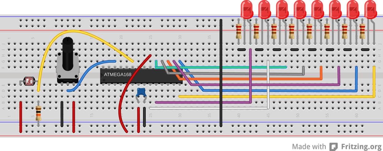
Figure 7-8. AVR night light circuit

You should also have at least a few of the LEDs still hooked up to this circuit so that you can see when the light is on or off. If you’d like to power something more significant than a couple of LEDs, you’ll need to use a transistor or relay as a switch, but this way you could actually turn on a quite useful light automatically when a room gets dark. See Chapter 14 for more details on switching large loads with the AVR. Until then, you can think of the LEDs as a stand-in.

The Code

The code for this project is super simple. Basically, I just wanted an excuse to show you my favorite channel-changing, ADC-sampling routine. Have a look at Example 7-4.

Example 7-4. nightLight.c listing

// Quick and dirty adjustable-threshold night-light.

// ------- Preamble -------- //

#include <avr/io.h>

#include <util/delay.h>

#include "pinDefines.h"

uint16_t readADC(uint8_t channel) {

ADMUX = (0xf0 & ADMUX) | channel;

ADCSRA |= (1 << ADSC);

loop_until_bit_is_clear(ADCSRA, ADSC);

return (ADC);

}

int main(void) {

// -------- Inits --------- //

uint16_t lightThreshold;

uint16_t sensorValue;

// Set up ADC

ADMUX |= (1 << REFS0); /* reference voltage on AVCC */

ADCSRA |= (1 << ADPS1) | (1 << ADPS0); /* ADC clock prescaler /8 */

ADCSRA |= (1 << ADEN); /* enable ADC */

LED_DDR = 0xff;

// ------ Event loop ------ //

while (1) {

lightThreshold = readADC(POT);

sensorValue = readADC(LIGHT_SENSOR);

if (sensorValue < lightThreshold) {

LED_PORT = 0xff;

}

else {

LED_PORT = 0x00;

}

} /* End event loop */

return (0); /* This line is never reached */

}

In this example, I initialize the ADC inside the main() routine. By now, you’re not surprised by any of these lines, I hope. I also turn on all the LEDs for output. (With eight yellow LEDs on my desktop right now, this night light would actually work pretty well!)

The event loop simply consists of reading the ADC value on the potentiometer and then the light sensor. If the value from the light sensor is lower, it turns the LEDs on, otherwise it turns them off. That’s it! Too simple.

The reason for this night-light demo, however, is the function readADC(). I probably reuse this function, or something similar enough, for tens of simple ADC applications. Taking a channel number as an input, it applies the bitmask to change the ADC channel, starts a conversion, waits for a result, and then returns it. Simple, effective, and it makes simple ADC sampling from multiple channels relatively painless.

Summary

You now know enough about using the ADC to do some pretty complicated sampling. Free-running mode is great when you’re only interested in one channel and you’d like to always have a contemporaneous value available. Single-shot mode is great when you don’t need to sample that often, or if you’re switching channels a lot as we just did here. You know how to use all 10-bits of the ADCs sample or how to set the ADLAR bit to left-adjust down to an easy-to-read 8-bit value in ADCH. That’s going to cover you for most simple sensor sampling situations.

We’re not quite done with the ADC yet, though. In Chapter 12, I’ll demonstrate some more advanced signal-processing methods (oversampling and smoothing) that are useful for getting more resolution from the sensor for stable signals and for getting smoother outputs from noisy signals. We’ll also experiment around a little with signal conditioning—namely creating a frontend voltage divider to expand the voltage range over which you can read with the ADC, and adding in a DC-blocking capacitor and biasing circuit for use with input voltages that otherwise would go negative, like microphones and piezo sensors.