Practical Electronics: Components and Techniques (2015)

Chapter 11. Logic

In electronics, the term logic generally means a circuit of some type that implements a logical function. The logic circuit might employ some relays, as shown in Chapter 10. Or it might consist of multiple small- and medium-scale ICs containing logic components, such as gates or flip-flops. It can be as simple as a couple of transistors and some diodes, or as complex as a modern CPU with billions of circuit elements.

The study of digital logic can, and does, fill entire textbooks (some of which are listed in Appendix C), but the primary emphasis in this chapter will be on the actual physical components.

We’ll start with a look at the building blocks of digital logic in the form of TTL and CMOS ICs. We’ll also take a quick look at programmable logic, microprocessors, and microcontrollers. The chapter wraps up with an introduction to logic probes and other techniques for testing logic circuits, as well as some tips for working with digital logic components.

Refer to Chapter 9 for a description of the package types used with logic devices. Chapter 4 shows some techniques for soldering ICs to circuit boards, and Chapter 15 discusses printed circuit board layout considerations for logic devices.

There is no way that the various families of available logic devices can be adequately covered in just a single chapter. For example, a typical data book from a manufacturer of digital logic devices is a thick tome with anywhere from 400 to 800 pages. And that can be for just one logic family or class of devices.

There’s no need to dread a future of wading through data books and online comparison tables, however. The key is to understand the basics of digital logic and the Boolean algebra on which it is based. Once you can define what you need the logic to do, or what it is already doing, then picking the appropriate type of logic device is largely a matter of practical considerations involving supply voltages, input and output voltage levels, and operating speed. Get the logic nailed down first; then worry about how to implement it with actual components.

Logic Basics

Digital logic is the application of formal logic theory, namely Boolean algebra, to electronic circuits. Boolean algebra was introduced in 1854 by George Boole in his book An Investigation of the Laws of Thought, and it defined a set of algebraic operations for the values 1 and 0, or true and false. In Boolean algebra, the primary operations are conjunction (AND), disjunction (OR), and negation.

The notation used for Boolean algebra uses ^ for conjunction, v for disjunction, and ~ for negation. Thus we could write:

Z = (A ^ B) v C

which states that the value of Z is equal to the result of A and B or C. This is the same as:

Z = (A AND B) OR C

The Boolean AND and OR operations always have at least two inputs and a single output. A digital circuit is the physical embodiment of a Boolean equation, with symbols for an AND gate, an OR gate, and negation, as shown in Figure 11-1.

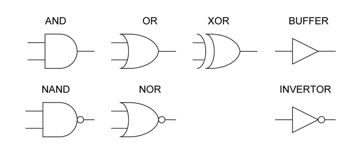
Figure 11-1. Common symbols for digital logic

The small “bubbles” used with digital logic symbols (as shown in Figure 11-1) indicate negation (or inversion, depending on how you want to think about it)—that is, if a logical true (1) encounters a bubble, it is negated and becomes a logical false (0), and vice versa. For example, Table 11-1 shows the truth table for an AND device (where A and B are the inputs).

The NAND (Not-AND) device, with a bubble on the output, produces the truth table shown in Table 11-2.

The buffer simply passes its input to its output, and it’s more of a circuit element than a logic operator. The invertor is a buffer with the output negated, such that a true input becomes a false output, and vice versa.

Don’t be confused by the open circles often used to indicate terminal points in a circuit diagram. These do not indicate logical inversion. Only when the open circle is next to a digital component symbol does it mean that logical negation is applicable.

Just as the NAND gate is the negation of the AND gate, the NOR gate is the negation of the OR gate. The XOR (which stands for exclusive OR) is not a conventional Boolean operation, but it shows up in digital electronics quite often. Figure 11-3 shows each of the gate logic symbols fromFigure 11-1 and its associated truth table. The buffer and invertor aren’t shown, because their functions are easy to understand.

Recall the simple logic equation shown earlier:

Z = (A AND B) OR C

Now consider Figure 11-2, which shows what the example logic equation looks like as a circuit diagram.

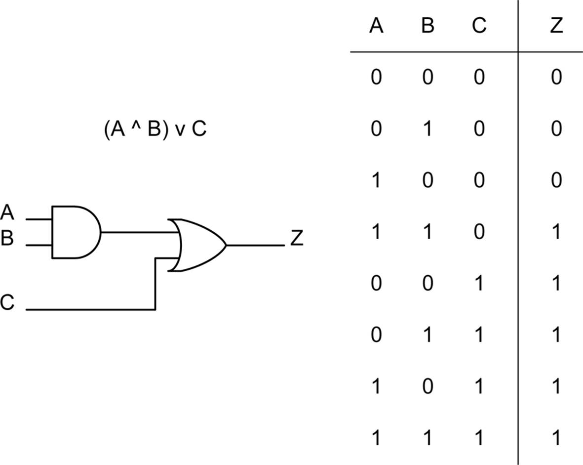
Figure 11-2. Circuit equivalent of (A AND B) OR C

The table to the right in Figure 11-2 is the truth table for this particular circuit. Truth tables show up quite often with digital logic designs.

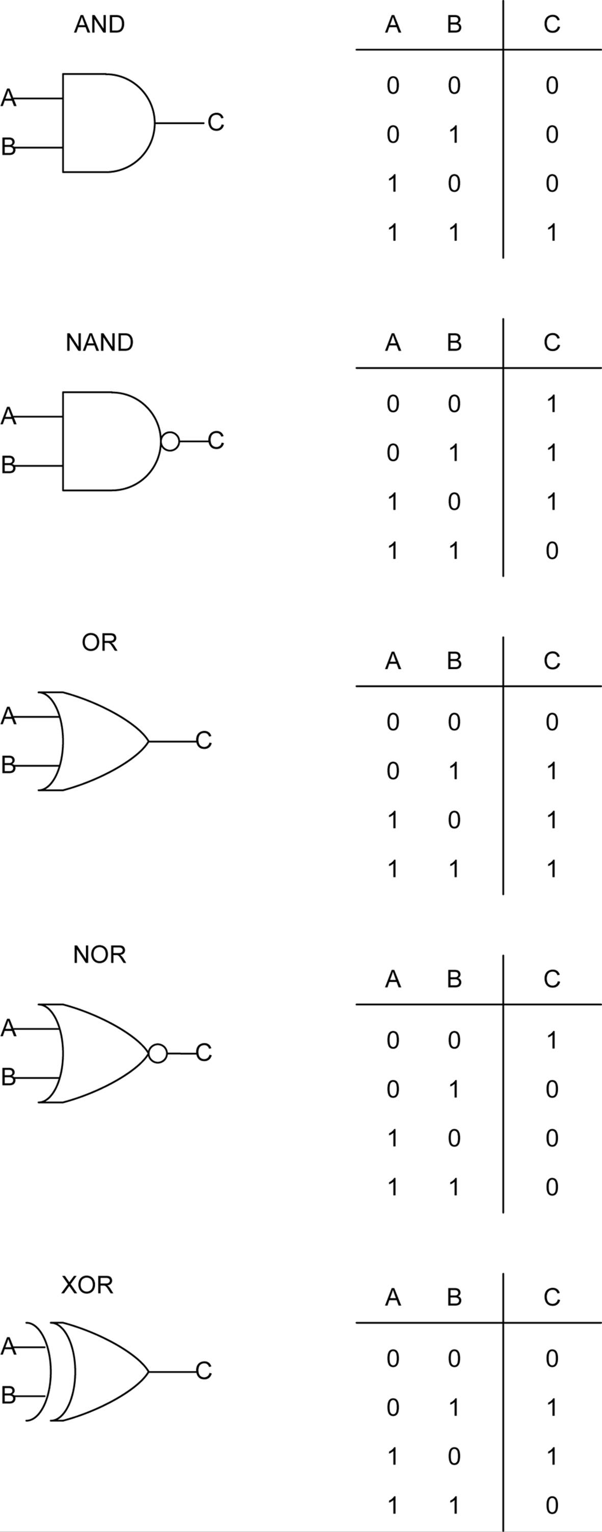
Figure 11-3. Truth tables for AND, NAND, OR, NOR, and XOR gates

Circuits that consist of the basic gates are called combinatorial logic, because they operate on combinations of inputs to produce a single output. Combinatorial logic has no state, except for that which exists instantaneously as a result of the input combination. When things like flip-flops are included in the mix, the result is referred to as sequential logic. A sequential logic circuit can have a “memory” of a previous state, and these types of circuits are found in things like state machines, counting circuits, pulse detectors, code comparators, and the CPU of a microprocessor or microcontroller.

An in-depth discussion of combinatorial and sequential logic circuits, while definitely an interesting topic, is beyond the scope of this chapter. Refer to Appendix C for sources of additional information.

Origin of Logic ICs

One of the drivers for the development of integrated circuits was digital logic. Early computers and logic systems utilized discrete components, initially with vacuum tubes and later with transistors. These were labor intensive to build, expensive to maintain, and expensive to operate, due to their power and cooling requirements. The development of the integrated circuit paved the way to smaller, faster, cheaper devices that used only a fraction of the power of the older designs.

An early form of logic gate, called resistor-transistor logic (RTL), was employed in the first commercial logic ICs that appeared in the early 1960s. The first computer CPU built from integrated circuits was the Apollo Guidance Computer (AGC), which incorporated RTL logic chips. These early RTL computers took human beings to the moon and set the stage for the electronics revolution that followed. Your smart phone, iPad, desktop PC, and the computer that runs your modern car can all trace their heritage back to something that had less computing power than a cheap MP3 player but was able to help guide a spacecraft from the earth to the moon, put a lander on the moon and then back into lunar orbit, and bring the crew safely back home again.

As time progressed, IC fabrication techniques continuously improved. This resulted in higher-density designs containing an increasingly larger number of components on the silicon chip. Early IC designs were called small-scale integration (SSI) and contained a small number of transistor components numbering in the tens of unique elements. The next step was medium-scale integration (MSI), where each IC might have a hundred or more unique circuit elements. Large-scale integration (LSI) is the term applied to IC devices with thousands of component elements on the silicon chip, and very large-scale integration (VLSI) is applied to devices with up to a million unique transistors and other circuit elements.

By way of comparison, early microprocessors had as few as 4,000 transistor elements. A modern CPU might have over 1 billion (1,000,000,000) unique transistor elements in its design.

Logic Families

In the world of digital electronics, types of devices are catagorized in terms of so-called families, referring to the underlying design and fabrication process technologies that are employed to build the logic devices.

The original logic families (which included RTL, DTL, and ECL, described momentarily) were derived from the logic circuits used in early computers. These early circuits were originally implemented using discrete components.

Today, there are four common families of IC logic devices in widespread use:

ECL

Emitter-coupled logic

TTL

Transistor-transistor logic

NMOS

N-type metal oxide semiconductor

CMOS

Complementary metal oxide semiconductor

For the most part, the two families you will encounter regularly are TTL and CMOS. ECL is still used for some specialized high-speed applications, but it is starting to become much less common. NMOS can still be found in some types of VLSI ICs, primarily CPUs and memory devices.

TTL is based on conventional BJT transistor technology, whereas CMOS employs FET metal-oxide-type transistors. Because the logic thresholds in CMOS devices are approximately proportional to power supply voltage, they can tolerate much wider voltage ranges than TTL. The bipolar devices used in TTL, on the other hand, have fixed logic thresholds.

CMOS devices can be implemented in silicon with very small dimensions, which has resulted in a rapid shrinking of CMOS chip size and a corresponding increase in circuit density per unit area. The reduced geometries, along with very small inherent capacitance in the on-chip wiring, has resulted in a dramatic increase in the performance of CMOS devices.

Logic Building Blocks: 4000 and 7400 ICs

The industry convention for naming monolithic IC logic devices is to use 4000 series numbers for CMOS parts and 7400 series numbers for TTL parts. Other logic devices have their own numbering schemes, some of which are standardized and others that are assigned by the chip manufacturer.

The members of the 7400 family of TTL monolithic IC devices and subsequent generations of parts in the 74Lxx, 74LSxx, 74ACTxx, 74HCxx, 74HCTxx, and 74ACTxx series are by far the most common basic units of digital logic. The older 4000B series CMOS devices are also still available and are useful in certain applications.

Closing the TTL and CMOS gap

Initially, TTL and CMOS devices had very different voltage and speed characteristics and couldn’t be used in the same design without some type of level shifting on the connections between devices. The reason for this is that TTL logic levels don’t rise high enough to be recognized as a logical 1 by a CMOS device. Table 11-3 shows the difference between the logic levels of traditional TTL and CMOS logic devices.

The compatibility issue was addressed with the introduction of the HC family of TTL-compatible devices. These parts have numbers with HC between the 74 and the TTL part number, and they are pin- and function-compatible with the original 7400 series devices. 74HC devices can be used with both 3.3V and 5V supplies.

The 74HCT family of devices was introduced to deal with the input-level incompatibility in 5V circuits. Internally, the logic is implemented as CMOS with TTL-compatible inputs. 74HCT devices work only with a 5V supply.

Table 11-4 details the CMOS and TTL families, by year of introduction.

4000 Series CMOS Logic Devices

When you are working with CMOS, either as part of the new design or when integrating to an existing circuit, it helps to have a selection of parts on hand. Table 11-5 shows a list of general-purpose CMOS logic devices that are handy to have around.

While it’s not absolutely necessary to keep a stock of parts on hand, it can save you time and money down the road when you really need something but can’t find it locally or don’t have the time to go run it down. Purchasing parts in bulk can also save a lot of money, so if you have some other people who might want to go in on an order, you can all realize the volume savings. Be sure to check out the resources listed in Appendix D for companies that sell overstock and surplus components.

CMOS parts are very static sensitive, so always take the appropriate precautions. Working on a antistatic workbench pad or grounded workbench, wearing an antistatic wrist strap, and removing a part from its antistatic packaging only when it’s absolultely necessary can help you avoid discovering that a small bolt of high-voltage static has punched a hole through the metal-oxide junction of a transistor inside a CMOS part and rendered it useless.

7400 Series TTL Logic Devices

If you plan on working with TTL-type logic on a regular basis, you might want to consider having a supply of 7400 series devices on hand. Table 11-6 lists general-purpose devices that cover the essential functions we’ve already discussed, as well as a few that can perform special functions, such as latching and buffering.

Most of the parts listed in Table 11-6 should be available as LS, ACT, and HCT types.

CMOS and TTL Applications

The disparity between CMOS and TTL has become less of an issue with each passing year. Some TTL devices are now basically CMOS logic with a 74xx part number. Microprocessors and microcontrollers are now built using low-voltage CMOS techniques and some types need low-voltage components to interface to them. The 74ACxx, 74ACTxx, 74HCxx, and 74HCTxx series of logic devices are essentially CMOS devices capable of operating at low voltages while still providing traditional TTL functions, and in the case of the ACT and HCT series, the ability to interface to conventional TTL devices operating at 5V.

So why would anyone want to buy a 4000 series logic device? A 4000 series gate has several unique features, such as high input impedance, low power consumption, and the ability to operate over a wide temperature range. For some applications, a 4000 series CMOS device can serve as an input buffer as well as a logic gate. For example, a level sensor for a water tank can be constructed with just a couple of 4000 chips, without any op amps. For more ideas of things to do with 4000 series logic, check out The CMOS Cookbook by Don Lancaster (listed in Appendix C).

What logic family to use largely comes down to what you want to interface it to. If you want to work with something that uses conventional TTL logic levels, the choice has largely been made for you. If you want to integrate a low-voltage microcontroller into a design, you might want to use CMOS parts for some of the “glue” logic in the circuit. There is no easy “if this, then do that” answer, unfortunately, and in the end it comes down to a series of design decisions based on operational parameters, project budgets, and interface requirements. And reading datasheets. Lots of datasheets.

Programmable Logic Devices

Programmable logic devices (PLDs) are ICs that contain unassigned logic elements and some means to configure the connections between them. Early PLDs used a form of fuseable link to determine how the internal logic elements would be arranged. The downside to this approach is that once a PLD was “programmed,” it would forever be that way. If the programming was wrong, or if there was a glitch during the process, the only recourse was to throw the part away and start over. There was no going back and trying again.

You can still purchase one-time programmable (OTP) PLDs today, and they are often used in production systems where there is a concern that someone might reverse-engineer a PLD and extract its programming patterns. Devices that can be cleared and reprogrammed utilize flash memory, UV EPROM (erasable programmable read-only memory) components, or some other technique to hold the programming data for the device.

There are four main types of PLDs in use today, as shown in Table 11-7. The PAL and GAL devices tend to be small and contain a limited number of logic elements. The CPLD-type parts are more complex, each being roughly equivalent to several GAL-type devices in a single package. The FPGA-type devices can be extremely complex and have the internal logic necessary to implement sequential logic designs, such as microprocessors, memory managers, and complex state machines.

The fundamental logic elements of a PLD, such as a PAL or GAL, are relatively simple. PAL devices have logic elements arranged as an array of “fixed-OR, programmable-AND” functional blocks. Each block implements “sum-of-products” binary logic equations. To get a basic idea of how a PLD works, consider the circuit shown in Figure 11-4, which is just a part of the internal logic found in something like a PAL device.

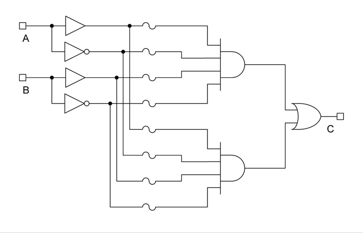
Figure 11-4. One part of the internal logic of a PAL or GAL device

Now, assume that we wanted to implement some logic, perhaps something like this:

C = (A ^ ~B) v (~A ^ ~B)

We can program this into the device by removing some of the fuseable links, which in turn allows only certain inputs to the AND logic elements, as shown in Figure 11-5.

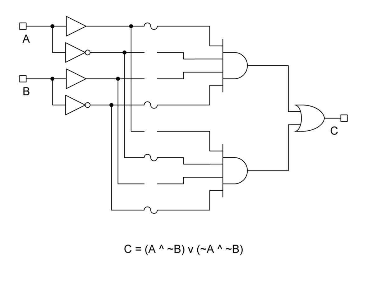
Figure 11-5. PAL logic configured to implement a logic function

A PAL or GAL device can help to significantly reduce the parts count for a complex logic design. For example, one way to implement the equation shown previously with conventional logic gates would require two AND gates, two inventors, and an OR gate. That would be at least three conventional logic chips, with some unused gates left over. The PAL does it in one logic unit, with other logic units on the chip available for other functions.

There is, of course, much more to PLDs than what has been presented here. Some device manufacturers provide free programming tools for their parts. These support the use of hardware definition languages such as VHDL, Verilog, and Abel. There are also websites that provide free IP cores or predefined FPGA logic in VHDL or Verilog, for things like microprocessors and I/O controllers (and more). The ARM microcontrollers that are found in smartphones, tablets, embedded controllers, and digital cameras are sold by ARM not as silicon parts, but rather as IP cores that can be implemented in silicon by the customer.

If you are interested in exploring this end of digital electronics, I would suggest getting a book like Kleitz’s Digital Electronics: A Practical Approach or Katz’s Comtemporary Logic Design (both of which are listed in Appendix C). The websites of manufacturers such as Altera, Atmel, Lattice, Texas Instruments, and Xilinx offer lots of free information about programmable logic devices in general and their products in particular.

Microprocessors and Microcontrollers

A modern microprocessor or microcontroller is the result of years of refinement in IC fabrication processes. Internally, most modern microprocessors and microcontrollers use CMOS fabrication technology, for the reasons of circuit density and speed mentioned.

The term microprocessor usually refers to a device that comprises the central processing unit (CPU) of a computer but which relies on external components for memory and input/output (I/O) functions. A microcontroller is a device that has an internal CPU, memory, and I/O circuits all on one chip. Nothing else is needed for the microcontroller to be useful.

To help clarify, consider this: an Intel Pentium-4 is a microprocessor, and an Atmel AVR ATmega168 (as found on an Arduino board) is a microcontroller. The Intel part is a CPU, with memory management, internal instruction cache, and other features, but it needs external memory and I/O support (also known as the support chipset). The AVR chip, on the other hand, has an 8-bit CPU, 16K of internal memory, and a suite of integrated configurable I/O functions.

Microcontrollers are much easier to work with than microprocessors because, for many applications, all that is needed is the chip itself. In fact, most popular small, single-board computers are really nothing more than a microcontroller with some voltage regulation and USB interface logic.

Unless you have a specific need to create a custom design around a specific microprocessor or microcontroller, it makes more sense to buy a prebuilt module. In terms of low-cost boards, there are the Arduino units based on the AVR family of microcontrollers and numerous boards that use some form of the 32-bit Cortex-M3 ARM processor design. Figure 11-6 shows two different boards that use the STM32 processor from STMicroelectronics. Low-cost microcontroller boards are also available for microcontrollers such as the Texas Instruments MSP430 and Microchip’s well-known PIC series.

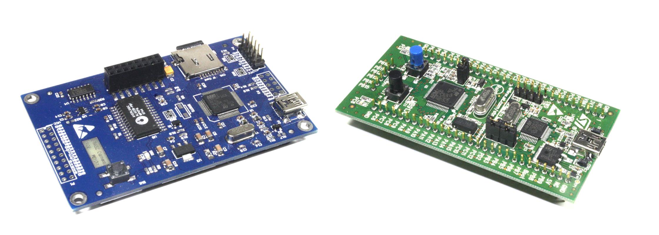
Figure 11-6. Two different STM32 ARM Cortex-M3 single-board computers

If you really need something with PC capabilities, many low-cost motherboards are available that use microprocessors from Intel, AMD, and Via. You can also find single-board PCs that are designed to connect to a common backplane (a so-called passive backplane that usually has just a set of edge connectors for PCBs to plug into), but these are generally intended for industrial applications and can be rather pricey.

Programming a Microcontroller

There are a couple of ways to get a microcontroller to do what you want it to do, and both involve programming. The first is by creating a sequence of instruction codes that the microcontroller can interpret and execute directly. Normally, you do so using a tool called an assembler, and the technique is called programming in assembly language. In the early days of microprocessors and microcontrollers, this was the primary way to program them, because languages such as C didn’t exist when these devices first appeared in the early 1970s.

Assembly language consists of a sequence of human-readable operation codes, or op codes, that an assembler converts into the binary values that the microcontroller will recognize and act upon. Op codes can have one or more associated values (called operands) for things such as a literal data value to load or an address in the program to jump to and resume execution.

Programs written in assembly language tend to be small, fast, memory-efficient, and difficult to read or modify. For example, a snippet of assembly language to read an incoming character from an input port might look something like Example 11-1.

Example 11-1. Example assembly language code snippet

INCHR: LDA A INPORT ; get port status

ASR A ; shift status bit into carry

BCC INCHR ; no input available

LDA A INPORT+1 ; read byte from input port

AND A #$7F ; mask out 8th bit (parity)

JMP OUTCH ; echo character now in A

Now imagine this expanded to hundreds, thousands, or even tens of thousands of lines. Assembly language can be difficult to write and difficult to read, and it doesn’t readily lend itself well to modular programming techniques (although it can be done with some discipline). In other words, assembly language programming can be hard to do well, so it’s no surprise then that this type of programming is now relatively rare. While in some cases it still makes sense to write low-level programs in assembly language, the advent of the C programming language provided for the second primary way to program a microcontroller.

C is an interesting language. It has been called “assembly language in disguise” by some, and one of its creators, Dennis Ritchie, once made the statement that “[C has] the power of assembly language and the convenience of…assembly language.”²

The C language also has the advantage of portability. Assembly language programs will work with only one type of processor, but a C program can often be recompiled to work on many different types of processors. Most modern operating systems are written in C (or another portable language) with only small machine-specific parts written in assembly language for a particular microprocessor.

A good modern C compiler will generate code that, while perhaps not as “tight” and memory-efficient as an equivalent assembly language program written by a skilled programmer, is still respectable. The ability of a compiler to create efficient and compact code depends to a large degree on the microcontroller that will run the resulting program. Some microcontrollers, such as the original 8051 family, can be difficult to use with C because of the limited amount of internal RAM (256 bytes). Others, such as the AVR devices found in Arduino products, are easier to work with and include instructions that allow a C compiler to generate fairly efficient code.

Types of Microcontrollers

These days, most microcontrollers come in 8-, 16-, or 32-bit types. Some, such as the Atmel AT89 series and the Cypress CY8C3xxxx family, are based on the venerable 8051 design created by Intel in the early 1980s. Others incorporate an ARM or MIPS 32-bit core in their design. Still others, such as the Atmel AVR series and Microchip’s PIC processors are unique, and are available in 8-, 16-, and 32-bit variations. Table 11-8, Table 11-9, and Table 11-10 list some common examples of each type.

Selecting a Microcontroller

The type of microcontroller that is most suitable for a particular project depends primarily on processing speed, on-board memory, and the type of I/O functions required. To a lesser extent, the selection decision might also be influenced by ease of programming and the availability of free or open source development tools.

As a general rule of thumb, if all something needs to do is control a motor or two, or perhaps just collect data and pass it along, an 8-bit microcontroller might be more than sufficient. A device like the AVR ATmega168, found on Arduino boards, runs at around 16 MHz and has I/O functions such as analog input and PWM output. The software tools to program the device are open source and freely available.

If, on the other hand, you need to control a color LCD display while capturing image data with a digital camera, a 32-bit microcontroller running at 100 MHz or more would be more appropriate. It could also be more expensive.

Although many of the 32-bit microcontrollers can execute instructions fast enough to run Linux (the Raspberry Pi, for example), speed isn’t everything, and it’s important to bear in mind that many things happen slowly in the real world. If there’s no need for speed, then don’t pay for it. Meeting the I/O requirements for a project is probably more important than worrying about how many instructions per second a microcontroller can execute.

The availability of programming tools is another key consideration. Before settling on a particular microcontroller, check to see what kind of development tools are available. If you’re planning to use something like a Raspberry Pi, Arduino, BeagleBone, or MSP430 Launchpad, see what the board supplier recommends. Also remember that a clone of one of these boards can usually use the same tools and techniques as an “official” board.

For microcontrollers like the AVR familiy, the MSP430, and the ARM-based chips, you can use Linux and the GCC toolchain to compile C or C++ code into binary code these processors can load and execute. There are also other open source compilers, linkers, and programming tools available for 8051-based devices. Microchip offers a free version of its development tools for the PIC microcontrollers.

Finally, unless you are familiar with JTAG and the interfaces used to program a microcontroller using that method, you might want to steer clear of some of the low-cost 32-bit ARM boards from Asia found on eBay and other places. There’s nothing wrong with these boards, but they typically show up in a bag or box with no CD and no documentation. It’s up to you to hunt down the details and fill in the blanks, and if you’re new to all of this, that can be a daunting task.

Working with Logic Components

In many ways, working with logic circuits is easier than with analog systems, if for no other reason than that the digital logic is, for the most part, electrically simpler. That’s not to say that it’s carefree, however, as there are some caveats and cautions that are unique to the world of digital electronics.

Probing and Measuring

Checking a logic circuit is relatively simple, because the various signals will be in only one of two states: on or off. Figure 11-7 shows a tool made specifically for this purpose.

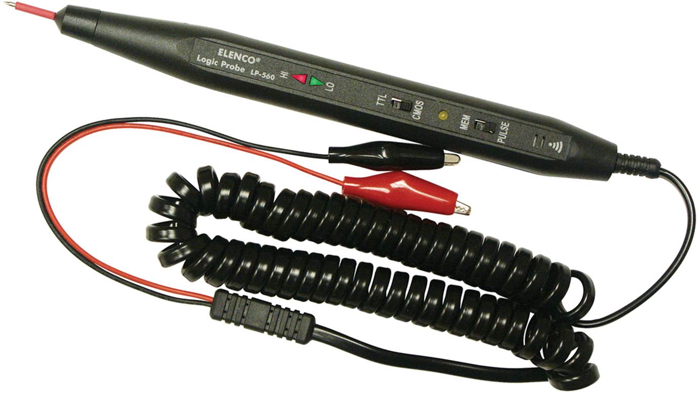
Figure 11-7. Hand-held digital logic probe

Using this tool is straightforward. You first connect it to the DC supply for the circuit using the red and black alligator clips. When you place the probe tip on the pin or lead of one of the circuit components, the lights on the probe will indicate if the signal state is high, low, or pulsing. Switches on the probe allow you to select for TTL or CMOS logic levels and also capture and display the last logic state, or specifically detect a signal that consists of pulses.

When using a DMM to measure signal voltages in a logic circuit, bear in mind that a typical DMM generally won’t show anything reliably except a static (or slowly changing) voltage. If you attempt to measure a signal made up of fast pulses, you might see some small amount of DC voltage, and the AC scale on the meter might show that something is there, but neither measurement mode will be accurate.

To accurately measure a digital signal, you need an oscilloscope, and to observe the behavior of multiple digital signals simultaneously, you really need to use a logic analyzer. Chapter 17 discusses both types of test instruments.

Tips, Hints, and Cautions

The following are some general tips, hints, and cautions to keep in mind when buying logic components and building digital circuits.

Selecting Logic Devices

§ Avoid selecting oddball or discontinued parts, unless you really don’t care about building any more similar gadgets in the future. Fascinating logic devices have come and gone over the years, but once that super-cool combination gate/adder/latch thing you’ve found goes out of production, or the stock at the surplus vendor runs out, you won’t be able to buy any more of them.

§ Purchase only what you are comfortable working with, both in terms of logic functions and physical package types. You can always go back and revise your design later on.

§ When building a circuit that uses devices from different logic families, always check to make sure that they are electrically compatible before actually acquiring them.

Physical Mounting and Handling

§ When using through-hole parts, consider using a socket unless there are space and cost constraints. A socket makes it easy to change out a part if needed, and sockets are particularly useful with EPROM or EEPROM memory devices.

§ Use good electrostatic discharge (ESD) prevention techniques. Work on a grounded mat, and use a grounded wrist strap.

§ Never install or remove an IC while power is applied to the circuit.

Electrical Considerations

§ When connecting multiple logic devices to a single device, take into account the current sink and current source ratings of the parts.

§ Make sure that parts are interface compatible. Older TTL parts cannot be directly connected to older CMOS parts.

§ Avoid connecting a logic IC input directly to Vcc (V+). Making the connection through a low-value resistor (between 220 and 480 ohms) is safer.

§ Never directly connect the output of a logic IC to either ground or Vcc.

§ Ground the inputs of unused gates and flip-flops. If left to float, the internal logic can change states or even go into oscillation, and this can induce spikes on the power supply lines.

§ Use decoupling capacitors at each logic IC. A 0.01 μF part is typical. The decoupling cap should be connected between the Vcc and ground pins on the device, and it should be as close to the device as possible.

Electrostatic Discharge Control

Static charges are the mortal enemy of solid-state components. Devices based on CMOS technology are particularly susceptible, but any solid-state device can be damaged under the right conditions. ESD control includes safe practices for component storage and handling.

The first step is to obtain and wear a grounded wrist strap when working with static-sensitive parts. You can pick up a decent production-line-grade wrist strap from most electronics suppliers, or you can order one (or several) online. Even one of the cheap things sometimes found at computer supply outlets will work in a pinch, but don’t expect it to last very long. Read and follow the instructions for connecting the strap to ground. Some straps have a built-in resistor to limit current, but some don’t. Some have an alligator clip to connect to a metal ground, while others use a banana-type plug.

The second item is a grounded mat for the workbench. These mats are made of a conductive, high-resistance material that is intended to dissipate stray static charges. Like a wrist strap, a mat will have a lead that must be connected to a solid earth ground.

Lastly, if you plan to stock logic ICs, you really should have a supply of high-density anti-static foam sheets on hand. These are made of a black or dark gray material, usually about 1/4-inch thick. The idea is to push the leads of an IC into the foam. The foam contains carbon or some other high-resistance conductive material and prevents a potential difference between the pins of an IC. For this reason, you should pick up a piece of foam containing ICs with your wrist strap securely in place before removing any of the parts. This discharges the foam and any parts on it. Plucking a part from the foam without first making sure that there is no overall charge on it can put an IC in a position where some leads are grounded by your fingers while some are still in contact with the foam. The part is in grave peril at that moment, and it could get damaged by a static discharge through it from the foam to you.

Summary

A digital circuit is essentially the physical implementation of Boolean logic, along with some finite state machine theory and other concepts. It is also one of the fundamental technologies of the modern world, and without digital circuits, we wouldn’t have PCs, the Internet, engine controllers for our cars, or programmable thermostats for our homes.

While it’s not necesary to use solid-state components to build a digital circuit (see Chapter 10 for a couple of examples of relay logic), modern logic ICs are compact, consume very little power, and best of all, are cheap. In this chapter, we’ve looked at the two main families of digital logic ICs: TTL and CMOS. We’ve also examined some of the more recent hybrid devices that straddle the divide between TTL and CMOS by incorporating the ability to connect to either type.

¹ VDD = supply voltage, VCC = 5 V ±10%

² From Wikiquote, quoted in Cade Metz, “Dennis Ritchie: The Shoulders Steve Jobs Stood On,” Wired, 13 October 2011.