Practical Electronics: Components and Techniques (2015)

Chapter 13. Analog Interfaces

In the real world, things happen in more or less continuous ways. When you walk, you don’t take steps in discrete movements, but rather as a flowing series of motions (which has been described as “controlled falling”). When the valve for a garden hose is adjusted, it isn’t set to some discrete amount of water flow in gallons or liters per minute. It just gets set to produce an output that “looks about right,” and it would be very difficult to get it back to that same exact level on the following day. Digital electronics handle changes as discrete steps or values, not as a continuum; this difference in how numbers are handled leads to a need to translate from one domain to another.

Mathematics and computer science define two basic types of numbers: integer and real. An integer is simply a whole number: –5, 0, 1, 2, and so on. The real world is the domain of real numbers, and there are a lot of them out there. Between 0 and 1, for example, there is an infinite set of real numbers.

A real number can represent any value (a point) along a continuous number line from –infinity to +infinity. The set of real numbers can be further divided into rational and irrational numbers. The set of integers is also a subset of the set of real numbers.

Rational numbers can be expressed as the ratio of two whole numbers (such as 12/1, 6/4 or 2/40), which is why they are called rational numbers, not because they make sense. They can also be written in decimal notion (such 12.0, 1.5, and 0.05). Irrational numbers (such as pi or the square root of 2) are also in the domain of real numbers, but they cannot be expressed as fractions. The value of pi, for example, can be approximated with a fraction (22/7), but it is only an approximation.

An important concept to grasp here is that the set of real numbers is infinitely large. For example, consider the possible values between 0 and 1. In that range, you will find 0.0001, 0.45, 0.87, and 0.022, along with every possible value in between. No matter how finely it is divided, there are still more numbers. Such is the nature of the real world, which is why it is a challenge to convert the infinite range of real numbers into a form that a discrete machine like a computer can deal with and why you’ll never be able to get the flow rate on the garden hose exactly the same tomorrow morning as it was yesterday.

Interfacing with an Analog World

Real numbers present a serious challenge for electronic sensors in general, and digital systems in particular. When a sensor measures some physical phenomenon (like, say, the temperature of an oven), it must first convert the physical manifestation of the heat into a voltage or current level that corresponds the physical phenomenon. Hence, the output of an analog sensor is just that: an analog, or close approximation, of the physical event in another form. In this case, it might be a voltage level that serves as an analogy for the original physical phenomenon (heat).

For a sensor, the challenge comes in the form of resolution. Consider the possible temperature values as an oven goes from 432 degrees to 433 degrees. It’s not just 1 degree. Remember that there are an infinite number of real values between these two integers. Sensors are rated according to their measurement resolution, or how small of a degree of change can be reliably and repeatably detected. How much resolution is really necessary will depend on the system using the sensor. For a common kitchen oven, a resolution of +/– 1 degree is probably overkill (a cherry pie will cook just as well at 373.3 degrees as it will at 377 degrees, even if the cookbook does call for 375 degrees). But, for some applications, a more precise degree of measurement is essential.

From Analog to Digital and Back Again

A signal from an analog sensor is a continuously variable voltage or current. While this is fine for an analog electronic circuit, it won’t work with a digital system. The analog signal must somehow be converted into a form that digital electronics can work with, which means binary values. This involves the use of devices called analog-to-digital converters (ADCs). An ADC takes continuous samples of the analog input and generates a stream of digital values, one per sample.

But the act of conversion introduces a new set of problems. Because of the discrete numeric nature of a digital circuit, it is not possible to capture analog data and convert it into a digital form with a level of accuracy that will allow for a 100% faithful representation of the original signal. This effect, called quantization, arises as a consequence of obtaining or generating a sequence of measurements of a continuously variable signal at discrete points in time.

With analog inputs, any changes in the analog signal between sample events are lost forever, and the result is only as faithful to the original as the number of samples per unit of time permits. This is illustrated in Figure 13-1, which shows the difference between a signal sampled once every two seconds and the same signal sampled twice per second. Notice how the reconstructed result of the faster sampling rate is much closer to the original, but it is still not a 100% faithful reproduction.

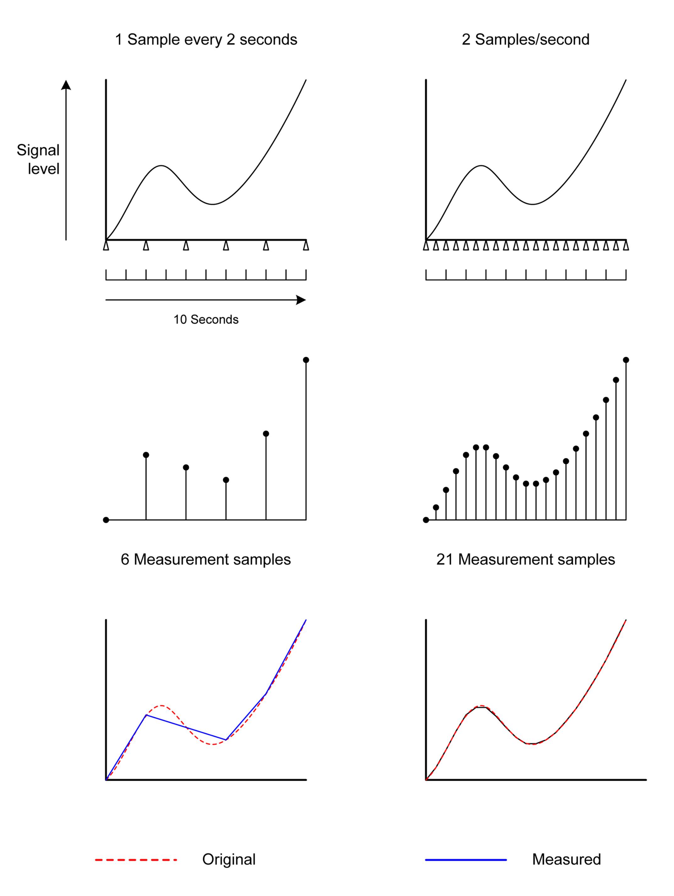
Figure 13-1. Effects of sampling rate on analog data digitization

Of course, not every situation needs a high level of fidelity in order to accomplish its objectives. In many cases, it is perfectly acceptable to take data samples at intervals of several seconds, or even minutes. This is particularly true when the measured input doesn’t change very much within the sample period, such as might be the case with something like the temperature in a greenhouse, the water level in a holding tank, or the temperature inside a house. Other cases, such as the conversion of audio to digital form, require very high sampling rates in order to accurately capture the highest frequencies of interest and maintain a high-fidelity representation of the original input. The sound circuits in modern PCs use a sampling rate of around 44,100 samples per second. Because of something called the Nyquist frequency (or Nyquist limit), the highest input frequency that can be accurately captured is half the sampling rate, or in this case about 22 KHz. We won’t delve too deeply into sampling theory here, but it’s worth looking into if you plan to work with audio or even higher frequencies.

Analog data is typically converted to digital form with a resolution (or data size) ranging from 8 to 24 bits per sample. Resolutions of less than 8 bits or greater than 24 are not readily available, but are possible. With an 8-bit resolution, the data will range in value from 0 to 255 (or from –128 to +127 if negative values are used). Again, not every application requires a high degree of precision, and sometimes less is more than sufficient.

When you are converting from analog to digital (or vice versa), there is an inherent limitation in the conversion referred to as quantization error. In general terms, this is the error between the original signal and the digital values (or codes) resulting from the conversion. As shown inFigure 13-2, the lower the resolution of the ADC, the more pronounced the quantization error becomes. The graph covers only the first eight samples, and the input in this case is linear (it’s a straight line). You can imagine it continuing on upward to the right, if that helps.

According to Figure 13-2 (which is only an approximation for purposes of discussion) a 9-bit ADC, with a range of 512 possible values (or codes), will generate a more accurate conversion than an 8-bit ADC with a range of only 256 possible values. The sampling events (the sample rate) are shown on the time axis as TS0, TS1, and so on. Note that it doesn’t matter if the 8-bit converter is sampled at a fast rate; it cannot do any better than its fundamental 8-bit resolution, although it will be able to detect and convert fast changes in the input that are within its resolution.

Sample resolution can be expressed in terms of volts/step, or, in other words, the measurable voltage difference between each discrete digital value in the converter’s resolution range. These are the codes mentioned earlier. Since ADCs generate binary codes instead of real-number values like 4.5 or 22.73, these codes must be translated into something that represents the original input voltage. This usually occurs in software, not in the ADC or the logic hardware. But in order to do the conversion, we need to know the scale. For example, if we have an 8-bit converter with a maximum full-scale input range of 0 to 10 volts, then each increment, or step, in the digital output code will be the equivalent of 0.039 volts. This can be expressed as:

§ Resolution = V_max/2ⁿ–1

Therefore, a 10-bit converter with a V_max of 10V can resolve 0.00978 volts/step, a 12-bit device can resolve 0.0024 volts/step, and 16-bit ADC can resolve 0.0001526 volts/step.

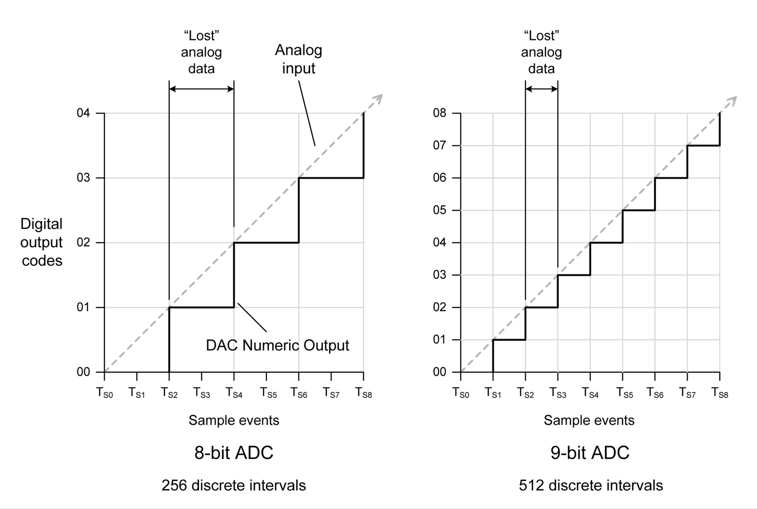
Figure 13-2. Analog input quantization

In Figure 13-1, the reason for the loss of fidelity between the sampling rates is a lack of samples to accurately track the changes in the analog signal in the slower example, not a lack of conversion resolution (the resolution isn’t even mentioned, actually). In Figure 13-2, it is the lack of resolution that results in the loss of fidelity due to quantization error. The sampling rate and the sample resolution together determine how accurately an ADC can convert an analog signal to digital form.

Lastly, there’s the issue of sensor error. If the analog input is noisy, or if the sensor produces an incorrect reading, it doesn’t really matter what the sample rate or resolution might be; the result will still be erroneous. For this reason, many circuit designs take pains to ensure that the analog inputs are as free from extraneous noise as possible. It’s common to use separate DC power inputs for the analog and digital sections of a circuit board so that the switching transients generated by the digital components don’t bleed into the analog sections. Sensor inputs can be shielded (seeChapter 7), employ twisted-pair wiring (discussed in Chapters 7 and 14, and incorporate filtering of some type to suppress high-frequency transients and noise (see Appendix A for information about filters).

Converting digital data into analog data is another challenge for digital electronics. The process basically involves generating a voltage output that corresponds to a digital value, and the more bits used, the better the fidelity of the output. The device for the job is called a digital-to-analog converter (DAC). Just as with an ADC, the DAC has some inherent limitations with regards to resolution, and the devices also exhibit quantization. Figure 13-3 shows the relationship between the resolution and the output update rate (or sample rate).

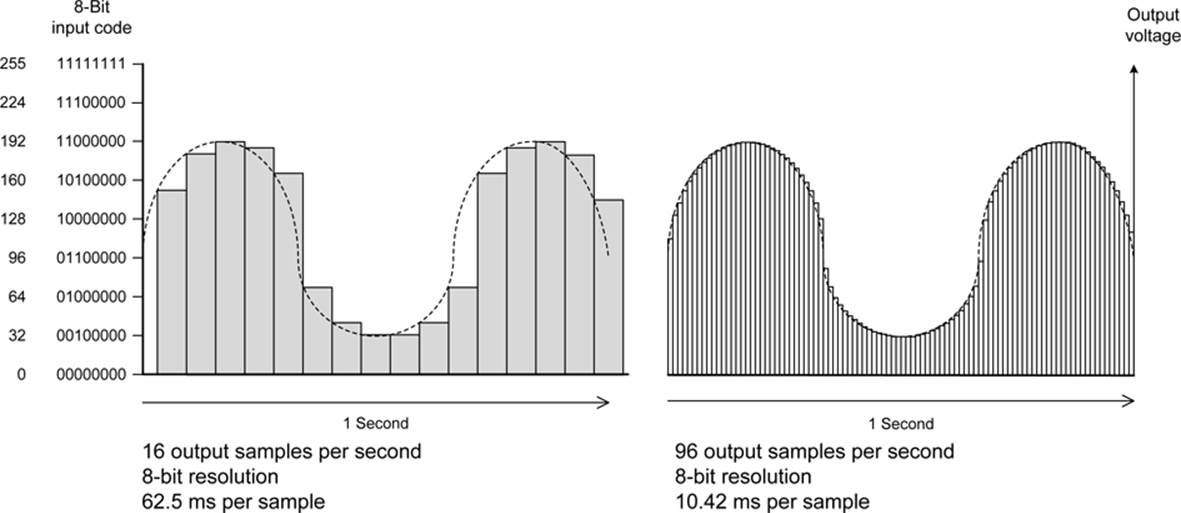
Figure 13-3. DAC output

For many applications, the output sample rate is not a critical parameter, and something on the order of once or twice a second between each output update will suffice. This is assuming, of course, that whatever the DAC is intended to control does not need to change at a faster rate. But, as you can see from Figure 13-3, the faster the output sample conversion rate, the closer the resulting output will come to the original input. Using a DAC with higher resolution (12 bits instead of 8, for example) will also improve the quality of the output. But, due to the effects of quantization, it will never be exact. This is one of the primary complaints of audiophiles who claim that analog media like phonograph records are more true to the original sound than an MP3 digital file. They may well be right, but I can’t hear the difference.

For some DAC devices, the output voltage range is established externally using a reference voltage. In other cases, the reference voltage is built into the DAC device itself. The output resolution is determined by the number of bits used to generate the output value and is just the output voltage range divided by the number of possible digital input values. The actual accuracy of the output is a function of the linearity of the DAC, with some types being more linear than others. Linearity, in this case, can be thought of as how well the DAC will generate a straight line output given a continuously increasing range of numeric values to convert.

It is possible to “smooth” the output of a low-resolution DAC by using a passive filter, but if you really need high fidelity, a high-resolution (16- or 24-bit) DAC is the way to go. If, for example, a 10-bit DAC is used, it will generate 1,024 discrete voltage steps across its output range. A 16-bit DAC is able to output 65,536 discrete steps.

Analog-to-Digital Converters

Many microcontrollers come with a built-in ADC (or two, or three). These might be 8- or 10-bit devices, with sampling rates based on a divisor of the basic clock rate of the microcontroller. In other cases, an external ADC is necessary, such as when you’re connecting to a PC or a microprocessor without a built-in ADC. An external ADC device can offer higher precision than a built-in function, and it can operate at a much higher sampling rate.

ADC devices come in the same packaging used with other types of ICs. Some types use a form of serial interface (I2C or SPI) rather than a parallel bus. This reduces the pin count on the device at the expense of conversion speed. Both through-hole and surface-mount packages are available.Figure 13-4 shows an inexpensive four-channel ADC module using an ADS1115 16-bit converter. This module can be used with any microcontroller or logic circuit that can support the I2C interface, and it can generate up to 860 samples per second. A similar module is available with a 12-bit converter for slightly less money.

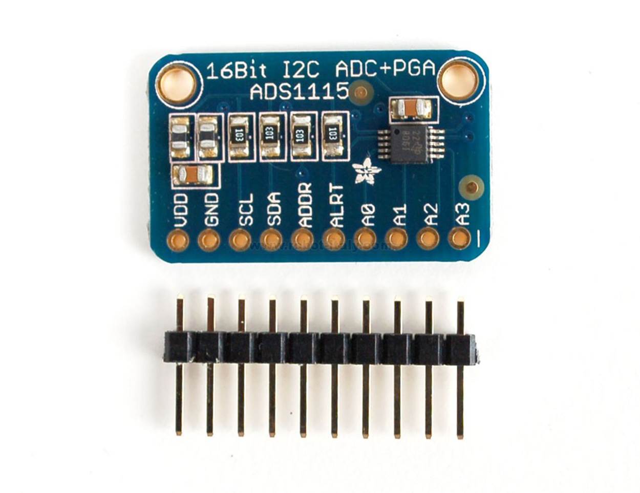
Figure 13-4. Four-channel, 16-bit ADC module (from Adafruit)

Another low-cost ADC is the MCP3008, an 8-channel, 10-bit device that uses an SPI interface and comes in a 16-pin DIP package. In fact, many good ADC ICs are available that require little in the way of control and data interface. They are easy to integrate into a circuit and simple to use.Table 13-1 lists some of the types available that utilize either the SPI or I2C interface.

When considering an ADC, either as a built-in function in a microcontroller or as a standalone part, keep in mind these key points:

§ Will the input voltage exceed the input range of the ADC? In some cases, this might damage the part, so it will need some type of voltage divider or limiter circuit to reduce the input level.

§ Will the ADC sample rate be sufficient for your application? What is the highest frequency you expect the ADC to measure? Or, put another way, what is the least amount of time between significant changes in the input? If the input changes significantly (perhaps 1/10 of a volt) only over the course of several seconds, you probably don’t need a fast ADC.

§ Carefully read and follow the IC manufacturer’s recommendations regarding PCB layout and power supply decoupling. This is particularly important when you are working with high-speed ADC devices, because they can be very sensitive to noise and voltage disturbances.

Digital-to-Analog Converters

Some microcontrollers include one or even two low-resolution DACs as part of their basic design, but many others don’t. DACs come in 8-, 10-, 12-, and 16-bit resolutions (and other resolutions, as well), and most built-in DACs will be in the 10- or 12-bit category.

Figure 13-5 shows a module with a MCP4725 12-bit DAC, suitable for use with any microcontroller capable of supporting an I2C interface.

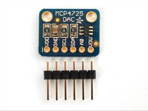
Figure 13-5. Single-channel 12-bit DAC module (from Adafruit)

Conversion speed is another consideration, but most modern DAC ICs are capable of operating up to 40 KHz or more.

With SPI or I2C devices, the two main parameters that effect conversion speed are the data transfer rate into the device over the serial link, and the settling time between discrete output levels.

Here are a few points to keep in mind when using DACs:

§ Don’t exceed the output current capacity of the device. If you need to drive something with a high current draw (e.g., a lamp or motor), use a buffer or driver device. Several high-current linear driver ICs (i.e., op amps) are available for situations like this.

§ If an output filter is needed, a simple resistive-capacitive filter might be sufficient (see Appendix A), but you might also want to consider an active filter of some kind. This has the added advantage of providing some degree of buffering to the DAC output.

Hacking Analog Signals

When confronted with an analog signal of unknown origin, you might be tempted to just toss an ADC on it and start measuring. But, before you do that, you need to make sure of a few key things.

When you are connecting to an unknown analog signal:

§ If you’re using an ADC that will work only with positive input voltages, verify that the signal won’t go negative. In other words, measure the signal while the device is active and observe the behavior.

§ Check the possible range of the analog signal. If you know the Vcc supply voltage for the external circuit, it’s usually a safe bet that it won’t exceed that.

§ Check to make sure the analog output can tolerate additional impedance loading. In other words, will the behavior of the alien device change if you connect your ADC circuit to it? If so, you’ll need to cobble up a high-impedance buffer to prevent unnecessary circuit loading.

If you need to isolate your circuit from the external circuit, you can use a transformer if the external signal is AC in nature. Small 1:1 audio and RF coupling transformers are readily available for applications like this. Another possibility is an active isolation circuit. Analog Devices offers an example in circuit note CN-0185. Note that this approach is not simple, nor is it something suitable for a novice. If you are dealing with a DC voltage that won’t change quickly, the circuit shown in Figure 13-6 might be suitable. Photosensitive resistors are described in Chapter 8.

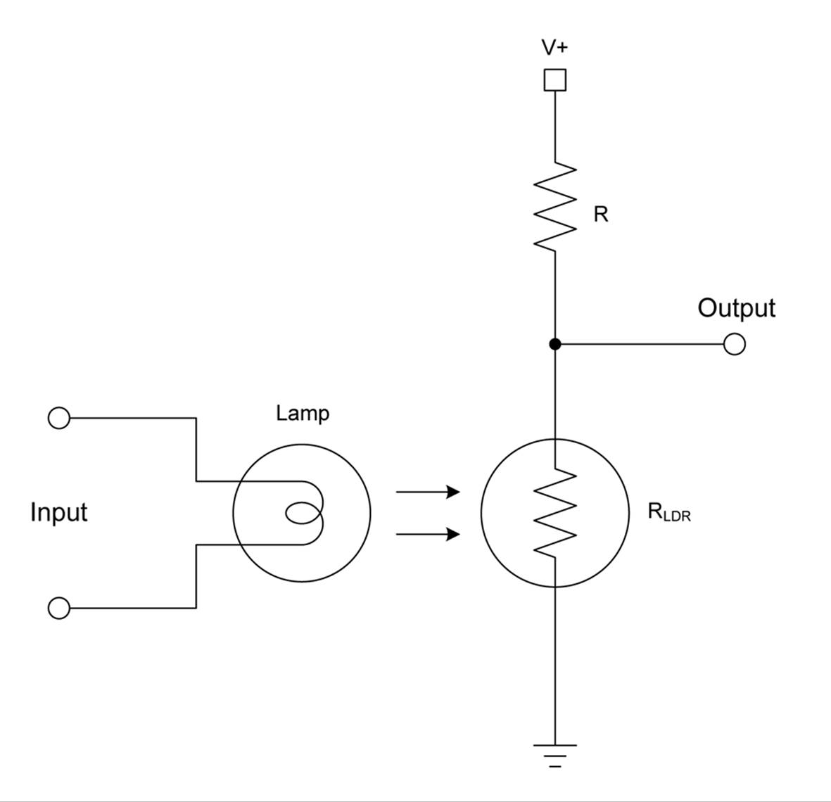
Figure 13-6. Simple low-speed signal isolator using a photoresistor

The circuit in Figure 13-6 employs a conventional miniature incandescent lamp, like a so-called grain-of-wheat type (because that’s about how large it is). The entire assembly can be encased in a short section of heat-shrink tubing, just like the homemade opto-isolator shown in Chapter 12.

Why a light bulb? Because an incandescent lamp has a continuous output response to input voltage. An LED, on the other hand, will start to glow only when the voltage reaches a threshold and it starts to conduct. In other words, the lamp has a continuous response while the LED is discontinuous.

As the amount of light falling on the photoresistor (also called a light-dependent resistor, or LDR) increases, its resistance decreases. In this circuit, the output voltage will fall as the input voltage driving the lamp increases. If that’s not what you want, you can swap the positions of R_LDR and R. Although simple, there are some points to consider with this circuit. First, is the input voltage suitable for the lamp? If it’s too high, you’ll need to add a voltage divider (discussed in Chapter 1) to adjust the input to the lamp. If it’s too low, you might want to consider some kind of amplifier (which is beyond the scope of this chapter but is covered in several of the excellent texts listed in Appendix C). Second, the value of R will depend on the range of R_LDR, and it should be such that the maximum current through the LDR under maximum illumination does not exceed its rating or cause it to self-heat. Check the datasheet for the LDR to see its limits. Lastly, this circuit is not linear, and the dynamic range will depend on the value or R_LDR, R, and how the lamp is driven. Before you attempt to use it, it would be a very good idea to connect the lamp to a battery, a potentiometer, and a DMM and calibrate the output as a function of the input voltage.

Connecting a DAC to an external device is sometimes fraught with peril. If you have the schematic for the device you are trying to hack, it should be possible to figure the optimal means to make the connection. If not, you’ll need to do some detective work to find the best way to gain control of the device.

Here are some final DAC hacking tips:

§ Try to determine the current draw of the external circuit the original analog signal is controlling. You can do this by inserting a DMM in series into the circuit and looking at the current display while the circuit is active. If it’s more than what your DAC is rated for, you might need to try to find another place to tap into the external device. You might be looking at the output of a high-current driver. Alternatively, you can use your own high-current driver to inject your DAC signal.

§ You shouldn’t try to “piggy-back” your signal on top of an existing analog control signal. The reason is that if your DAC is trying to output a high voltage level, and the external circuit is trying to pull the analog signal low, there could be some excessive current flow. You can build a simple DC mixer circuit with an op-amp and a few resistors, but it’s still better to have just one analog voltage source active at a time. See The Art of Electronics (listed in Appendix C) for some circuit ideas.

Summary

This chapter provided a quick tour of the world of analog-to-digital conversion and back again. This is a field that has its own reference books, and what has been presented here is just the top of the waves when it comes to things like quantization, sampling rates, resolution, and other topics. However, the up side is that, for many applications that don’t involve audio, video, or radar systems, you can just pay attention to the voltage range and the conversion resolution.

There are other types of ADC and DAC devices in addition to the ones listed here. The parts highlighted here were chosen because they have a simple interface that is easy to work with when you’re using something like an Arduino, BeagleBone, Raspberry Pi, or similar microcontroller-based board. However, if you want to build your own control logic from the ground up, you might want to consider the ADC and DAC components that provide access via a parallel data bus. These devices offer high resolution and high-speed conversion rates but at the cost of more complicated control and data transfer circuitry.

To learn more about analog-to-digital and digital-to-analog conversion, refer to the excellent texts listed in Appendix C. You can also glean a lot of useful information from the Internet, at the websites of component manufacturers in particular.