Practical Electronics: Components and Techniques (2015)

Chapter 17. Test Equipment

This chapter is a quick tour of what is available in the way of inexpensive test equipment, starting with the ubiquitous digital multimeter (DMM) and moving on to oscilloscopes, signal generators, and logic analyzers. The focus here is on low-cost tools that will help get the job done without costing a small fortune. In the world of test equipment, it’s all too easy to spend a lot of money, with some types of equipment running upward of $30,000 each (or more). For the vast majority of situations you are likely to encounter when working with common electronics components and devices, that sort of precision and processing speed isn’t necessary.

Now would probably be a good time to talk a bit about things like speed, accuracy, and bandwidth. We’ll cover these topics in more detail later on in relation to each type of instrument, but the main point is that, for the vast majority of things you might want to build or modify, you don’t need an oscilloscope with a bandwdith capable of displaying a 1 GHz signal, nor do you need a digital meter with 4 1/2 digits of resolution. You don’t need an RF spectrum analyzer, or a high-precision pulse generator, or even a frequency counter. When you are working with things that interact with the real world in some fashion, the times involved are typically anywhere from 10 to 1,000 ms (0.01 to 1 second). Physical things usually don’t move much faster than that. If you are working with a microcontroller, it will be running at a much faster rate, but you don’t have visibility into the chip itself, just the inputs and outputs, and they are slow by comparison to the microcontroller’s internal clock.

Basic Test Equipment

This section describes the two most fundamental types of test equipment: the digital multimeter and the oscilloscope. With just these two instruments, you can design, test, debug, and hack a wide range of electronic circuits. In fact, even an oscilloscope isn’t absolutely necessary in many cases, but a DMM is essential.

Digital Multimeters

A modern DMM can be used to measure voltage, current, and resistance. Some models also include the ability to measure capacitance, inductance, and frequency, among other things. These devices are available in both portable (hand-held) and bench versions. There are also rack-mount variations for permanent installations.

DMMs are available in a range of prices depending on resolution, accuracy, and any additional features. Some basic models are available from around $10, although they might not offer much in the way of accuracy or functionality. Other models that feature increased accuracy, better measurement resolution, and enhanced features can range in price from about $30 to upwards of $300 or more.

If you have nothing else, the one thing that is essential is a decent DMM. Typically, the low-cost models are hand-held devices, designed for portability and battery operation. Figure 17-1 shows a basic DMM, and Figure 17-2 shows a fancier (and more expensive) model.

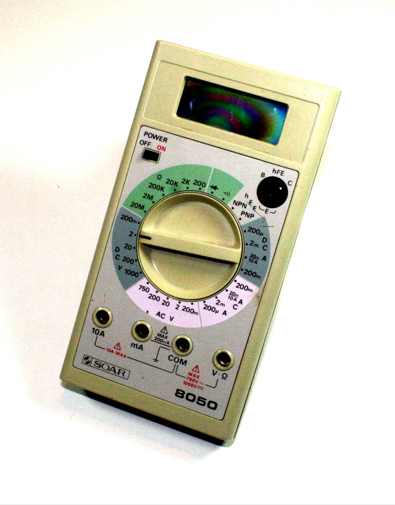
Figure 17-1. Basic low-cost DMM

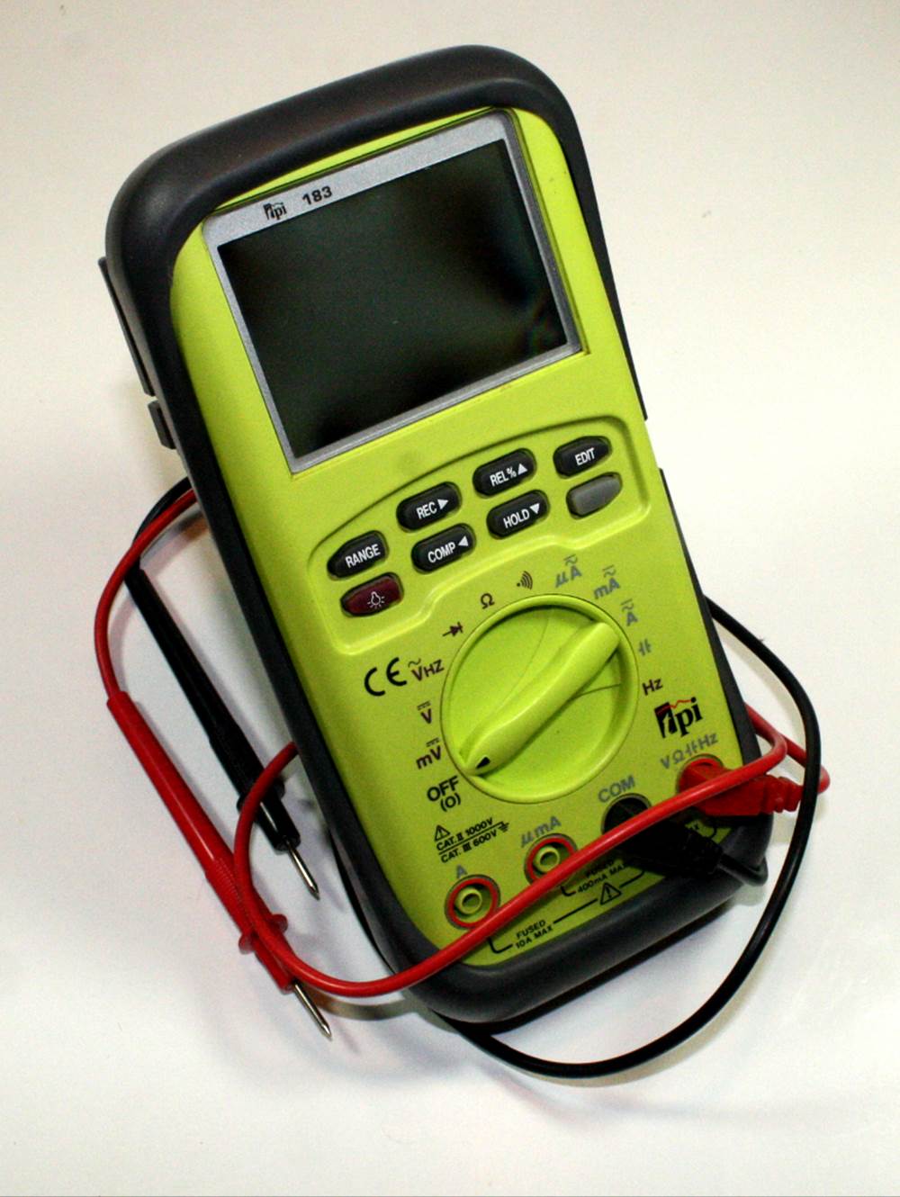
Figure 17-2. DMM with enhanced features

The two main criteria for a DMM are resolution and accuracy. The resolution of a DMM is reflected in how many digits the device is capable of displaying. A meter with a 3 1/2-digit resolution will not show some very small values, but a meter with a 4 1/2-digit resolution will. The 1/2 refers to the most significant digit on the display, which is typically a 1. A meter that can display from 19,999 to 0.0001 is a 4 1/2-digit resolution device, and a 3 1/2-digit DMM can display from 0.001 to 1,999. Low-resolution meters tend to round measured values to fit in their display resolution range. So a voltage of 0.0006 V would show up as 0.001 V on a 3 1/2-digit meter, assuming that it rounds up.

Using a DMM

When poking around in a live circuit with a DMM, you can encounter a range of voltages. The DC supply will, of course, read at or near its design value. At other points in the circuit, the voltage will be less than the supply level. This is due to resistances and semiconductor junctions. Also, looking at an AC signal with a DMM set to the DC input will often show some small amount of voltage. This could be some DC present with the AC. If you think you should be seeing more than the DMM is showing, try switching to an AC input. If the signal is within the DMM’s frequency range, you might see a higher reading for the AC component in the circuit.

Always check the settings on a DMM before touching the probes to a live circuit. Bad things can happen if the probes are placed across a high voltage while the meter is set to measure resistance or current.

Although the negative probe (usually black) of the DMM can be connected to the local ground, with battery-powered meter, it doesn’t have to be. You can measure the voltage drop across a resistor by touching the probes to either end of the part. This technique can be used to determine if any current is actually flowing through the resister: if there is no voltage drop (the voltage across it is zero), then no current is flowing.

Never attempt to measure resistance in a live circuit. The DMM generates a small voltage when measuring a resistance, and this can wreak havoc with an active circuit. The DMM can also be severely damaged if you do this.

Measuring resistance with a DMM is straightforward, but be aware that measuring a part’s resistance while it’s in a circuit might give an erroneous reading, depending on what other parts are in the circuit.

To get a truly accurate measurement of small values of resistance, you should first touch the probe tips to each other and hold them tightly. If the DMM is capable of reading a small resistance, you should be able to measure the resistance of the probe leads. Subtract this from whatever reading the meter shows to get the actual resistance of the item between the probes. Note that some meters have the ability to automatically compensate for probe lead resistance.

Measuring current usually involves changing the connection of the positive (red) lead from the V input jack to the A jack. The meter in Figure 17-1 has two current input jacks: one for low-level readings and the other for up to 10A. Notice on the rotary dial that it can also measure both DC and AC current. The DMM shown in Figure 17-2 is essentially the same.

When using a DMM to measure current, it is important to bear in mind that the meter itself is part of the circuit. With a voltage measurement, it’s more of a passive observer, but with current, it becomes directly involved. The reason is that a DMM uses an internal shunt resistance for current measurement. The shunt is a precision, low-ohm device (often just a piece of metal) that will exhibit a small voltage drop when current flows through it. The meter is actually reading the voltage drop across the shunt. To the external circuit, it appears as a conductor with a very low resistance.

Let’s say, for example, that you wanted to know how much current is being used by a circuit designed to operate from a battery. Figure 17-3 shows one way to do this.

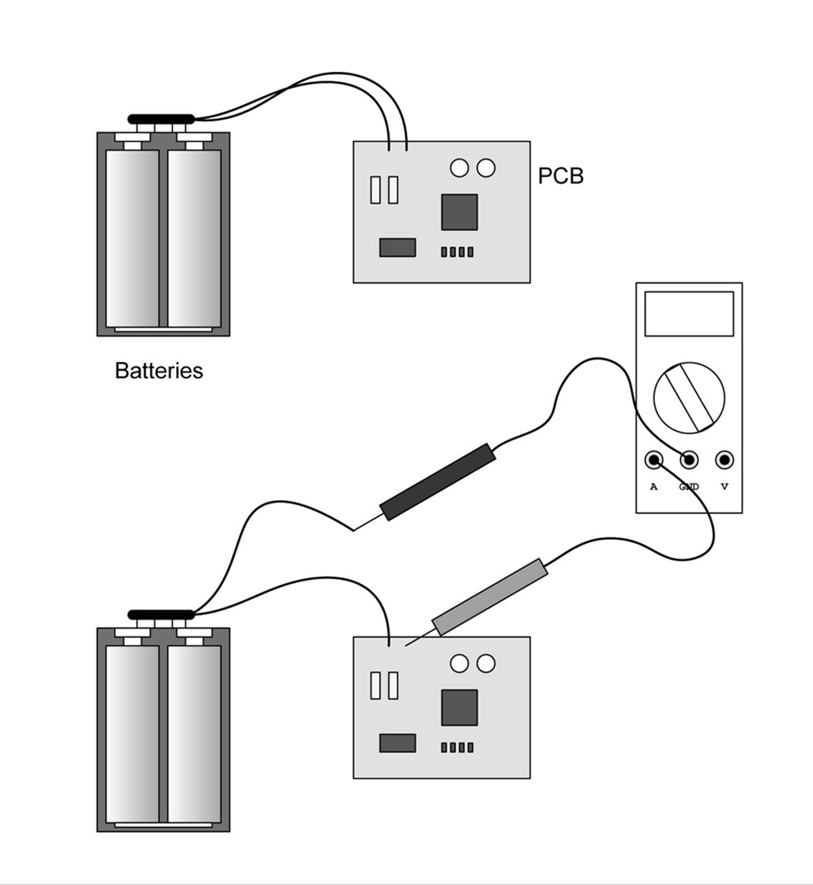
Figure 17-3. Measuring the current consumed by a circuit on a PCB

In order to measure the current used by the PCB, one of the leads from the battery pack will need to be disconnected. The DMM is then inserted between the battery and the PCB. An alternative approach would be to make a special cable with the appropriate connectors to allow it to be inserted between the battery pack and the PCB. It might even have a pair of banana-type plugs already connected to plug directly into the DMM.

When the DMM is configured to measure current, never connect it directly across a power source. Most better models have an internal fuse, but that isn’t always guaranteed to protect the meter from a fast voltage transient. And even if the fuse does sacrifice itself to save the meter, it can be a pain to replace the fuse on some DMMs.

Oscilloscopes

An oscilloscope measures changes in voltage over time. That’s it, but it doesn’t really need to do anything else. By measuring an input signal over time, you can determine the voltage level, the frequency (if it’s a periodic signal), and the rise and fall time of the start and end of a pulse. By using a current shunt (a type of low-value resistor), an oscilloscope can also measure current as a DC voltage across the shunt.

An oscilloscope is a versatile piece of test equipment that allows you to see what is going on inside a circuit. There are some models available that are about the same size as a smartphone. In fact, some are built into cases that look like smartphones, like the one shown in Figure 17-4. They typically won’t work with high-frequency signals, but they’re fine for looking at relatively slow events. The device shown in Figure 17-4 cost about $50 from a Chinese vendor through eBay.

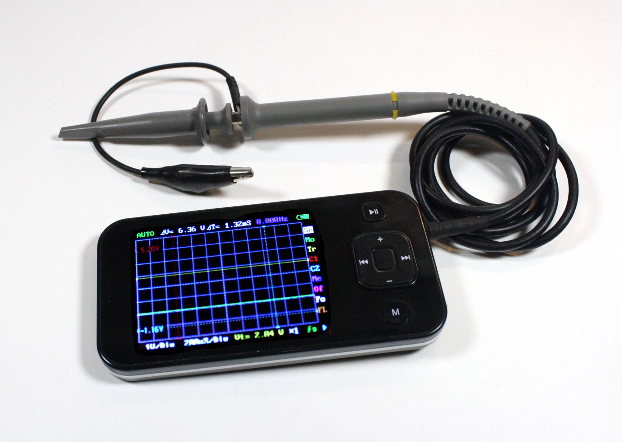
Figure 17-4. Miniature digital oscilloscope

Some oscilloscopes use a PC as the display. These devices plug into a standard USB port and serve as the front end to convert the external signals into a stream of data that a special application running on the PC can display as a waveform. If you elect to purchase a USB oscilloscope, make sure to read the specifications carefully, paying special attention to the sample rate. For example, one unit might sell for the amazing price of $34, but it might measure signals only up to 3 KHz. Another might sell for $70, but it might measure signals up to 20 MHz. Figure 17-5 shows one type of low-cost USB oscilloscope. Generally, these units are all variations on the same theme: small plastic enclosures with two BNC connectors for the probes and a USB connector (usually a type B). Some have additional indicators and controls, and the high-end units might have more memory to store the digitized waveforms.

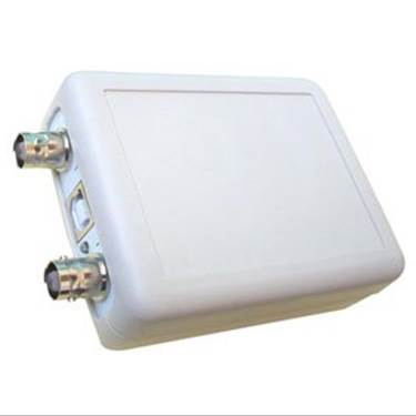
Figure 17-5. USB digital oscilloscope

You can use even the sound system in a PC as a low-speed oscilloscope by applying the signals from a circuit (with some appropriate buffering and protection) directly to the microphone or line inputs. Figure 17-6 shows one such application for Linux (xoscope).

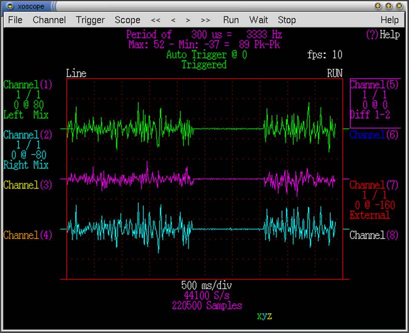
Figure 17-6. xoscope running on Linux (image from http://xoscope.sourceforge.net/)

While something like xoscope might seem like a neat idea, be aware that it usually won’t measure DC voltages (it depends on the type of audio input used in a particular PC). Why? Because a capacitor on each audio input prevents DC from getting in. Also be aware that it won’t measure signals with a frequency greater than 22 KHz, because the audio input will not respond to anything higher than that (it’s limited by the maximum sampling rate of the audio input analog-to-digital convertor in the PC). Check out the official xoscope home page for more details, and if you elect to install it, be sure to read the manpage.

It is also possible to use an Arduino as the hardware frontend for a digital oscilloscope running on Linux. Figure 17-7 shows the display window of the lxardoscope application. lxardoscope isn’t particularly fast; in its basic configuration, its sampling rate limits it to around 1.5 KHz.

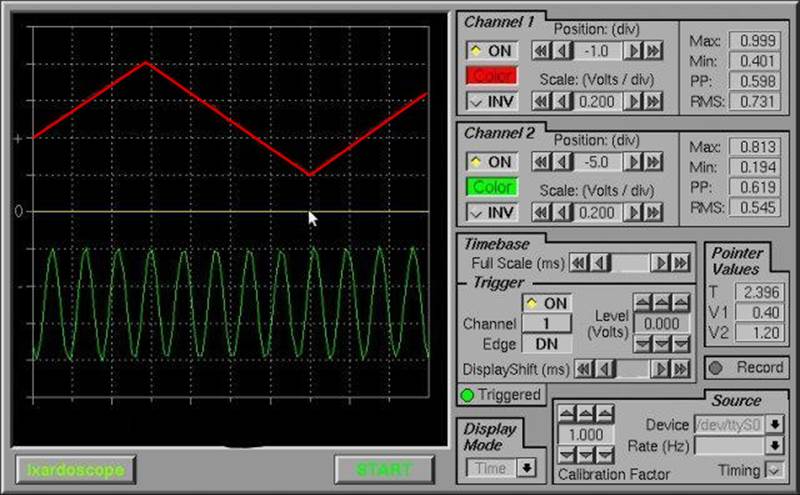
Figure 17-7. lxardoscope running on Linux (image from http://sourceforge.net/projects/lxardoscope/)

Be forewarned that this is something you’ll need to compile yourself, and the Makefile that comes with it is set up for a 32-bit platform. To compile it to run on a 64-bit Linux machine, you will also need to install the libforms2 package. It won’t hurt to install the libforms-dev andlibforms-doc packages as well. Replace the reference to the included libforms.a library in the Makefile with -lforms and add -m64 -march=x86-64 -fPIC to the CC_OPTIONS declaration.

Also note that you’ll need to build a pre-amplifier circuit, so this falls under the catagory of major project. Still, it’s an interesting example of how to integrate different subsystems into a functional whole, and I’ve included it for that reason. The archive from Sourceforge comes with documentation, schematics, and other interesting technical data. If nothing else, it’s worth a look to see how someone else solved a particular problem.

If you would prefer something already built and tested, benchtop portable digital oscilloscopes capable of measuring waveforms up to 25 MHz are available for around $300. But if you really need a faster instrument, be prepared to pay upward of $1,000 for it, and some brands and models can be even more expensive. A web search for “digital oscilloscope” will return over 3.6 million results. That’s a lot of shopping to do. Figure 17-8 shows an example of a compact portable digital storage oscilloscope.

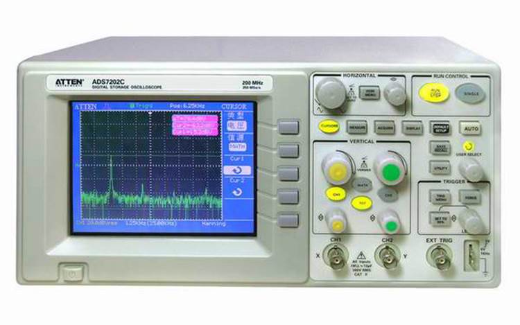
Figure 17-8. ATTEN ADS7202C digital storage oscilloscope

How an Oscilloscope Works

Oscilloscopes were invented early in the 20th century, when radio engineers realized that they really needed to be able to see what their circuits were doing. A voltmeter just didn’t work for some situations. These early tools used a glass tube, similar to an old-style television picture tube, to display a dot that moved across the screen from left to right at a rate determined by a knob on the front of the instrument. Another knob was used to adjust the gain (also called sensitivity) of the input to keep the signal within the vertical limits of the display. Figure 17-9 shows a generic block diagram for an analog oscilloscope.

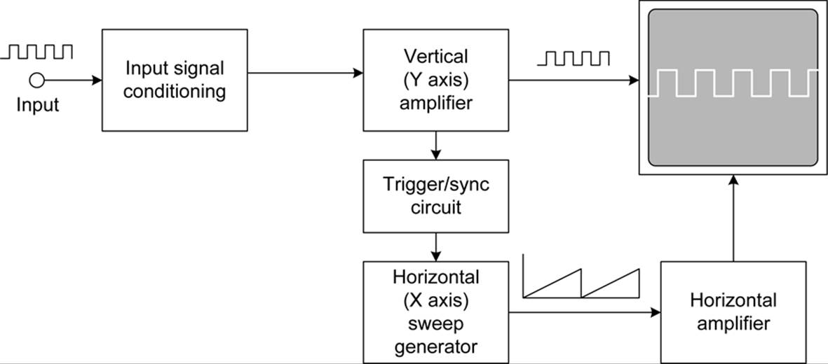
Figure 17-9. Old-style (analog) oscilloscope block diagram

A basic old-style analog oscilloscope consists of a vertical amplifier/converter, a trigger/synchronization circuit, a horizontal sweep oscillator (or timer), and some type of display, typically a cathode-ray tube (CRT, similar to an old-style TV or computer monitor glass display).

The idea is to cause the display to respond to the input signal by moving the display point up or down as it sweeps across the face of the display. In older instruments with a glass CRT, the beam of electrons that creates the spot on the face of the tube is literally steered across the display while being deflected up or down by the vertical input signal. If you get the chance to work with an older CRT type oscilloscope, you should do so. It will help make some of the concepts masked by digital instruments much clearer.

Being able to see an input waveform is good, but if the horizontal timebase isn’t in sync with the signal, it will appear to drift (or wander) across the display. The trigger circuit is used to lock the horizontal timing to the input and create a steady display. A trigger circuit works by sensing when the input signal has reached some threshold. When this occurs, the horizontal timebase is effectively reset to make the input signal appear to stand still in the display. Changing the horizontal sweep rate while the trigger is active has the effect of magnifying the input waveform in the horizontal direction. This allows you to zoom in on an interesting part of the waveform.

With a good trigger and a known hortizontal sweep rate, you can determine not only the peak-to-peak level of the input waveform, but also the frequency. Older instruments had a clear plastic plate over the face of the CRT with a grid machined or molded into it. Lamps along the side of the plate (hidden behind the bezel around the CRT) were used to illuminate the grid lines. Determining the frequency of the input was simply a matter of counting the number of vertical lines between repeating peaks in the waveform and multiplying by the time per division as determined by the horizontal rate.

The early oscilloscopes were all analog. Modern oscilloscopes are digital, meaning they convert the input signal into a stream of binary numbers (Chapter 13 describes analog-to-digital convertors). The binary data is used to generate a waveform on an LCD display. In a digital oscilloscope, the display processing is done virtually by the internal microprocessor after the signal is converted from analog to digital. Figure 17-10 shows a block diagram for a modern digital oscilloscope.

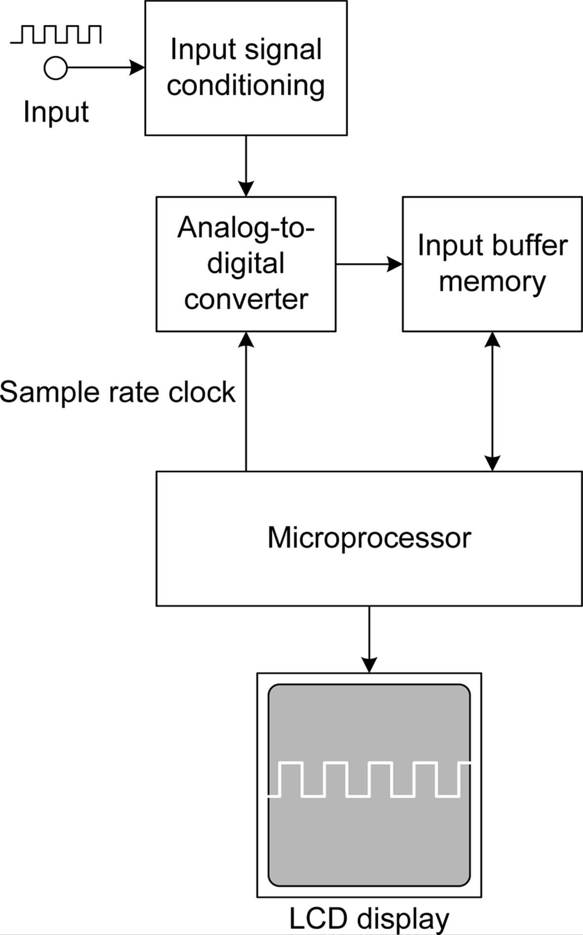
Figure 17-10. Digital oscilloscope block diagram

In modern digital oscilloscopes, measuring the frequency of the input signal is typically one of the functions done automatically by the input conversion and display logic in the instrument. A digital oscilloscope will also display the peak-to-peak level of the input signal, and many digital instruments have the ability to position cursor bars in the display to measure a particular part of a signal, such as the rise time of a pulse or the voltage level of a particular part of a waveform. Figure 17-11 shows the display generated by a digitial oscilloscope. This particular model doesn’t have an LCD display, but it’s otherwise fully solid-state and completely digital.

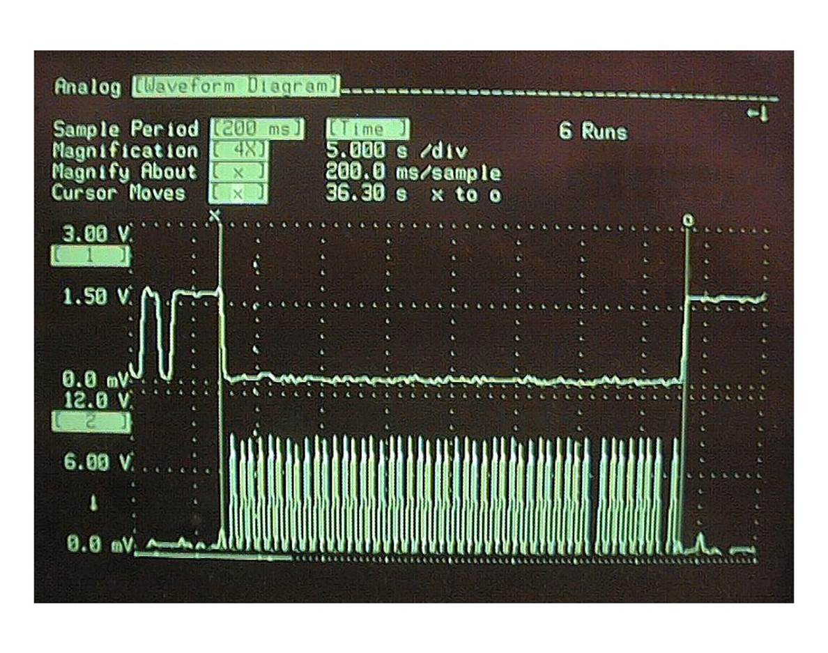
Figure 17-11. Digital oscilloscope display

Using an Oscilloscope

As mentioned earlier, what you will be able to measure with an oscilloscope depends on how fast the instrument can respond to the input. This is largely a function of how fast the horizontial oscillator can run, but it also depends on the frequency response characteristics of the input amplifier section.

I mention this because if you use a low-speed instrument to look at a high-frequency signal, you might not see what you would expect. In an old-style analog oscilloscope, the input will generally fall off as the frequency exceeds the upper limit of the vertical amplifier circuit, and what’s shown on the display will look like a solid bar or a fuzzy blur, if it shows much of anything at all. In a digital oscilloscope, the maximum input frequency is limited by the sampling circuit. A signal that exceeds half of the maximum sampling rate is subject to aliasing, which is a result of the Nyquist limit (a fundamental concept in sampling theory). An aliased signal will appear to be a different frequency than it really is, so other than demonstrating that there is really a signal present, it’s generally useless.

It’s really very simple to actually use an oscilloscope. Figure 17-12 shows a diagram of a generic modern digital oscilloscope.

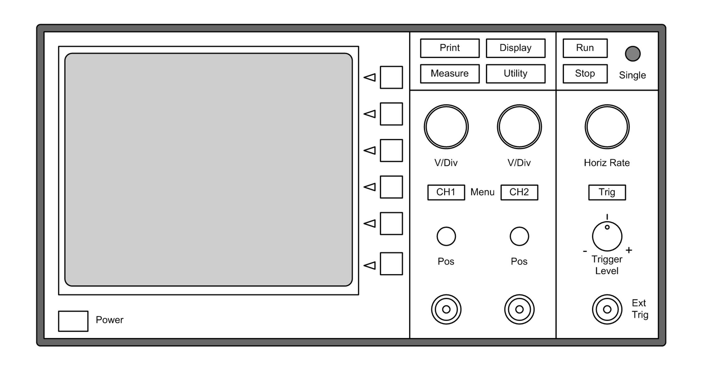
Figure 17-12. Generic digital oscilloscope front panel and controls

Here you can see that the instrument has two inputs, or channels. Each input channel corresponds to the vertical or y-axis input of an older analog oscilloscope, and each has a V/Div knob. This control determines the sensitivity of the input channel. Note that the control knobs operate in units of volts per division, where the division refers to the reference lines that appear on the display. You can see these in Figure 17-11. As you turn the V/Div knobs, the readouts on the display will change to indicate the active display range.

The buttons labeled Pos set the vertical position of the waveform on the display. You can adjust these to move a waveform display to where you want it and even have channel 1 overlap channel 2, which is sometimes useful when you’re comparing two inputs.

The next major section of the front panel is the horizontal control. In an analog oscilloscope, this would be the sweep frequency: the rate at which the beam is driven across the face of the display. In a digital oscilloscope, it is essentially the amount of time from one side of the display to the other. To view a waveform with a frequency of, say, 1 MHz, you could set the horizontal control to around 0.00001 seconds (10 microseconds). That would be 1 microsecond per division if there are 10 divisions on the display. You should then see 10 cycles of the input waveform.

The last primary knob is the trigger level. As mentioned earlier, the horizontal rate of the display can be locked to the input signal. This results in a stable display that doesn’t wander or drift over time. The trigger works by sensing when the input signal has exceeded a particular threshold, either positive or negative. Adjusting the trigger level allows you to select a part of the waveform to use to synchronize the display, and a digital oscilloscope will generally show what the trigger is currently set to by using a moving horizontal line on the display or a numeric readout in the display, or both.

The buttons along the side of the display are used for things like math functions, input mode selection, reference marker selection, instrument setup, and so on. The CH1, CH2, and Trig buttons might call up menus on the display, and the side buttons allow you to make selections from the menus. These button might also have dynamic functions that are available while the instrument is running and acquiring data.

A real digital oscilloscope will have more controls than this simple diagram, but they are all basically the same. Some just have more bells and whistles than others. If you acquire or have access to an oscilloscope, be sure to spend a little time with the user manual (if one is available, of course).

Here are a few tips and cautions for using an oscilloscope:

§ Unless the oscilloscope is battery operated (as some modern digital oscilloscopes are), always use a grounded outlet. Leaving the chassis floating without a ground return can lead to situations where weird noise appears for no reason (it would most likely be a local AM radio station), or the chassis of the instrument can go hot and give a nasty shock, or even worse, cause a short and severely damage something (including you).

§ Always ground the input probe. That’s why it has a ground lead attached to it. With some oscilloscopes, the ground leads on the probes are connected to a common point inside the instrument, so you might get away with connecting one but not the other, but don’t count on this.

§ Never connect the ground lead on an oscilloscope probe to anything that isn’t actually ground. Some instruments are designed to allow this, but some aren’t, and it’s unpleasant to discover that the ground lead really is ground when connected to a DC voltage in a circuit.

§ With a digital instrument, be aware of potential aliasing. If you think you should be seeing a waveform at a particular frequency, but you are seeing something else, you might have exceeded the sampling limit for the instrument.

Advanced Test Equipment

At some point, you might find that you need something more than a DMM and an oscilloscope. When it comes to advanced test equipment, some of the most useful items are pulse generators, signal generators, and digital logic analyzers. These instruments can help wring out the kinks in a troublesome circuit and show what is going on at a specific moment in time.

But don’t rush out and buy them just yet. In order to get the most from test equipment like this, you really need to have a good reason for using it and a good knowledge of how to use it.

Pulse and Signal Generators

Pulse and signal generators are closely related, in that both can generate a repeating waveform. Typically, a signal generator will produce a sine wave, although one variation called a function generator will also output square, pulse, ramp, and triangle waveforms. A pulse generator isn’t designed to output anything other than pulses (as you may have surmised from the name), but it is good at what it does. A quality pulse generator will output a single pulse, a burst of pulses, or a continuous train of pulses, all at a specific duty cycle. Many units can be configured to emit one or more pulses when a trigger signal is detected, and some models have the ability to dynamically vary the duty cycle in response to a control input (pulse-width modulation).

A new bench signal or pulse generator will run $300 and up, depending on the features and the brand. Since these are not items in high demand, they tend to be on the pricey side. Physically, digital signal, pulse, and function generators all look more or less the same. They have controls to set the output frequency, perhaps a knob to adjust the pulse duty cycle (if pulses are provided), and maybe a digital display to show the frequency or time of the output. A function generator will almost always have controls to select the type of output waveform.

Just as there are low-cost versions of oscilloscopes and DMMs, there are low-cost versions of signal and pulse generators. Figure 17-13 shows an Arduino-compatible DDS (direct digital synthesis) module that is capable of generating waveforms from 0 to 40 MHz using a AD9850 DDS IC. The AD9850 chip on the PCB can generate both sine and square waves, and it is relatively easy to interface to an Arduino (or some other single-board microcontroller). Toss in an LCD display, some connectors, and a nice case, and it would make a usable programmable signal generator.

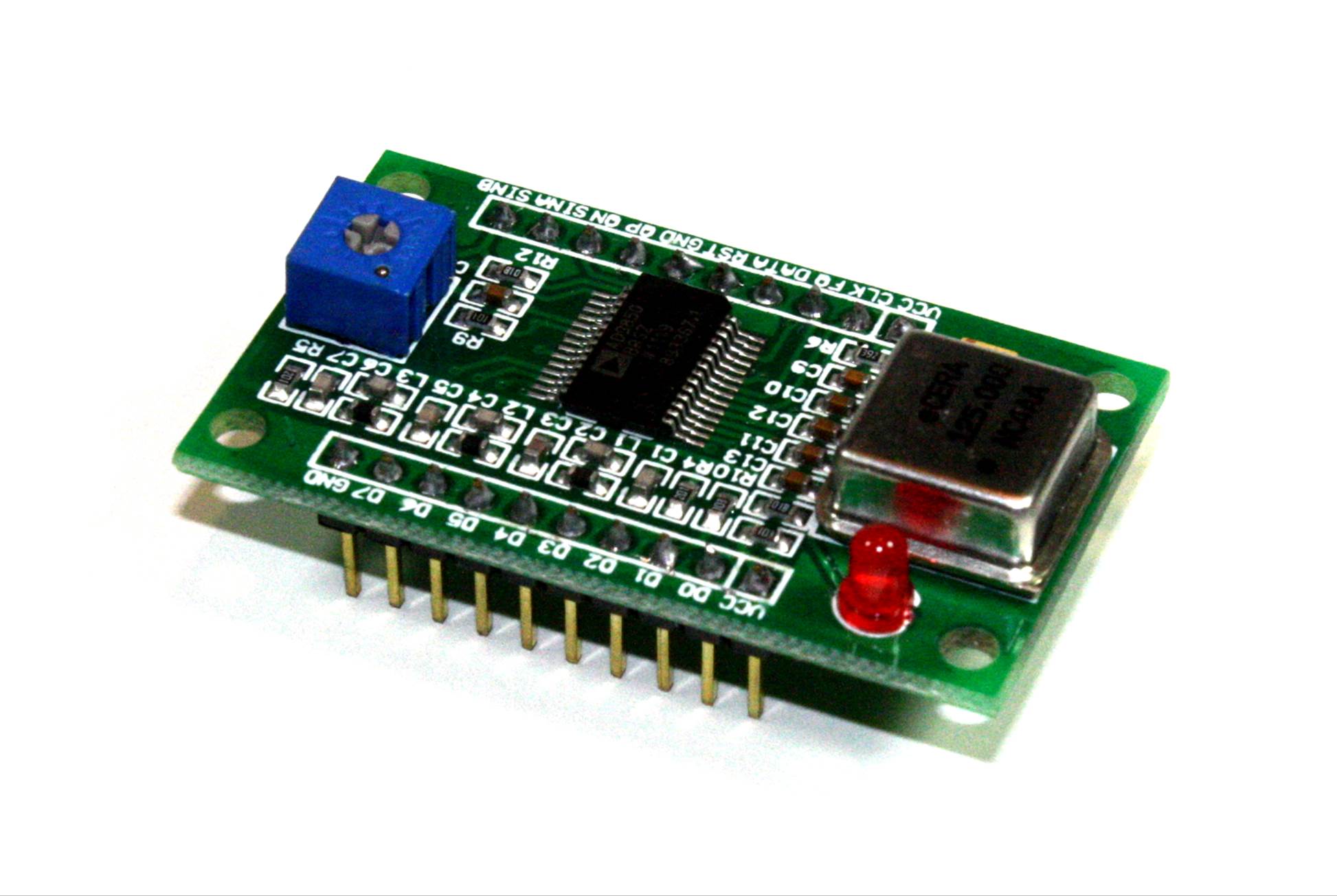
Figure 17-13. An Arduino-compatible AD9850 DDS module

If you’re interested in the AD9850, I would suggest downloading the datasheet from Analog Devices and studying it. It has a serial interface, but it uses a 40-bit internal register to hold a 32-bit frequency control word, a 5-bit phase modulation word, and a power-down function. That means it needs 40 bits of data each time the frequency or phase modulation is changed. This isn’t hard to do in software, but it is beyond the scope of this book. You can usually find example code on the websites where the module shown in Figure 17-13 is sold, and an article on the Instructables website describes how to build a cheap programmable sine wave generator using this module.

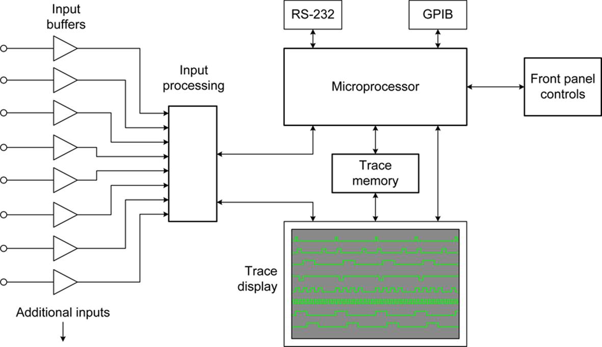
Figure 17-14. Simplified logic analyzer block diagram

Logic Analyzers

The logic analyzer is a useful instrument for measuring and monitoring activity within digital circuits. Logic analyzers capture a set of digital inputs simultaneously and store the binary values in a short-term trace memory. The contents of the trace memory are then read out and displayed in the form of a timing diagram. Figure 17-14 shows a block diagram of a simple logic analyzer. This diagram would be applicable to a self-contained instrument, but there are other ways to achieve a similar result. For example, if the signals are changing relatively slowly, you can use the parallel printer port on a PC as a simple four-channel logic analyzer (the PC parallel port has four input lines available).

So, what does a logic analyzer show you? Figure 17-15 shows an example of the timing diagram generated by a logic analyzer. The idea here is that every input channel has its own line on the display. When a channel input goes high, the trace line goes up, and when it is low, the trace line returns to its zero position. A logic analyzer is particularly useful for visualizing how signals are changing state over time, both independently as a result of the action of other signals in the circuit. Logic analyzers often have 8, 16, or even 32 inputs.

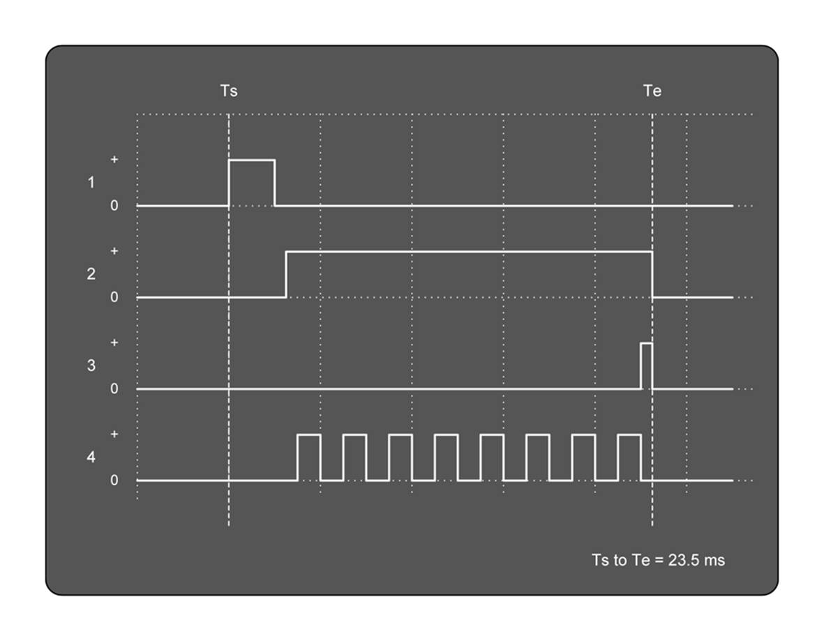
Figure 17-15. Example logic analyzer display

In Figure 17-15, you can see that a trigger (channel 1) causes the state of channel 2 to change to high, and at the same time, 8 pulses are generated (channel 4). After the eighth pulse, another signal (channel 3) occurs, which resets channel 2. What we have here might be a stepper motor controller moving the motor eight steps in response to an input trigger.

Also notice the Ts and Te vertical lines. Most logic analyzers provide some type of time reference markers that can be moved to different parts of the display. By using the reference markers, you can find out how long the trigger pulse on channel 1 was active, or the time between the falling edge of the trigger pulse and the start of the counter that generated the eight pulses. The digital oscilloscope display shown in Figure 17-11 is actually the oscilloscope function of a Hewlett-Packard 1631D logic analyzer, and you can see the X and O time reference markers on the display.

Some logic analyzers have the ability to display the data as a table of hexadecimal values, and still others have a built-in capability to observe and decode the signals used in a serial interface. Some can also be configured to start collecting and displaying data when a particular pattern appears on the inputs. What the instrument can do depends, to a large extent, on how much you are willing to pay for it.

Inexpensive USB logic analyzer modules are available that use the PC’s display rather than provide one of their own. Figure 17-16 shows a diagram of such a device.

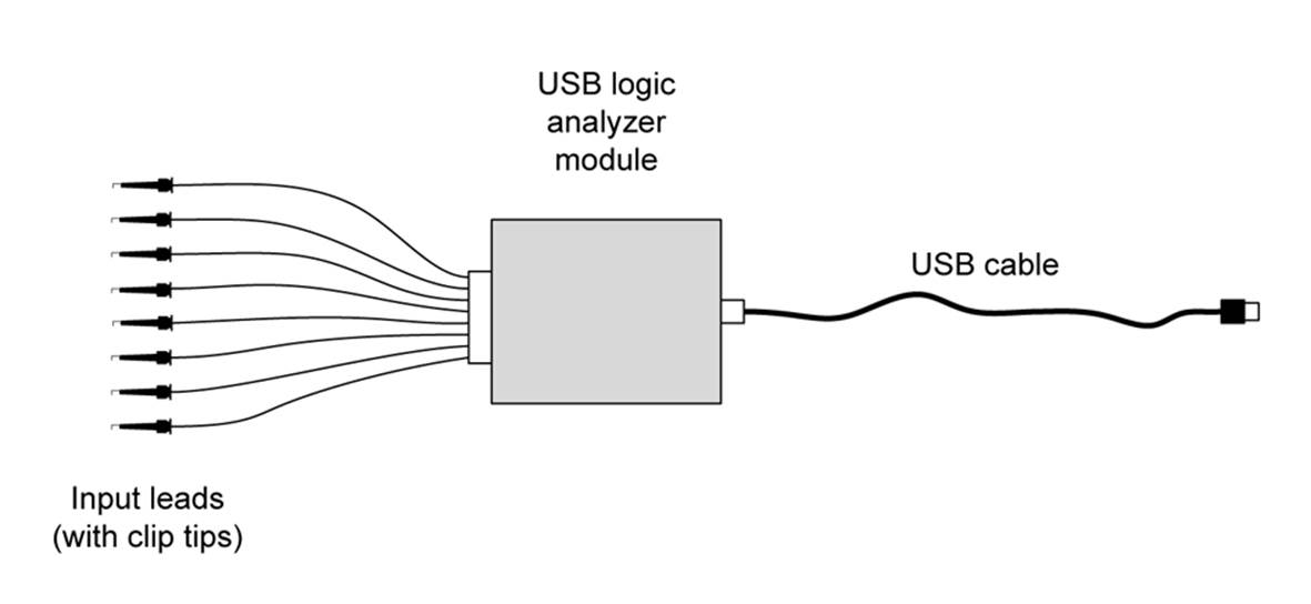
Figure 17-16. A simple USB logic analyzer device

Prices for USB logic analyzers vary, starting at about $150 and going up, depending on the built-in capabilities and number of input channels. The display used with these looks similar to the one shown in Figure 17-15. Keep in mind, however, that for $150 you’ll get something that can sample data at a maximum of about 3 to 5 MHz. If you need to look at faster signals or need more than four or eight inputs, be prepared to pay considerably more.

Buying Used and Surplus Equipment

It is possible to set up a decent electronics lab with only used equipment, if you are careful about what you buy. Used digital meters, oscilloscopes, signal generators, frequency counters, and other items are available from local surplus outlets (if you happen to be lucky enough to have one near you), some electronics supply shops, and, of course, eBay. Ham radio operators occasionally hold swap meets, and you can often find bargains on older gear at one of these events. Flea markets are another possibility, but more often than not, what they are selling is simply junk that might be good for parts, but not much else. If you happen to have an electronic manufacturer or a university in your city that holds surplus sales, you might find something worthwhile there as well.

With used equipment, you also need to be prepared to do some minor repairs and calibration work yourself. All of it works, and every item has a service manual on file, and all of it needed some kind of minor calibration and repair work. Having documentation for your equipment is essential. Without the service manual, it is very difficult, at best, to perform the calibration steps necessary, or hunt down and replace a defective component should one fail.

Yes, the cart looks a little rough, to be sure, but it will get a new paint job at some point in the future. The paint doesn’t make the equipment behave any better or worse, so it’s not really a high priority. If you’re curious, what you’re looking at here, in top-to-bottom order, is a Sony/Tektronix 338 logic analyzer/protocol analyzer, a Tektronix 454 dual channel oscilloscope, a Fluke 8000A DMM, a Fluke 1900A multi-counter, and a HP 3478A DMM. The black box is a passive backplane PC with a GPIB/IEEE-488 interface.

One last comment about this equipment: it’s slow. The oscilloscope is useful to only about 150 MHz, and the logic analyzer tops out at 20 MHz. But slow is OK. As stated earlier, most things, particularly things that interface with the real world, don’t move very fast. Another big advantage of slow equipment is that it is cheap. Those who think they just have to have an oscilloscope capable of looking at GHz signals will pass by the older unit selling for a fraction of the cost of the fancy instrument, even when it can handle 90% of anything they might want to do.

Here are a few more caveats about used test equipment:

§ Don’t buy anything with vacuum tubes in it, no matter how cool it looks. Instrument-grade vacuum tubes are almost impossible to find these days, they use a lot of electricity, and they get hot. Really hot.

§ Unless you are prepared to spend your money for something to use for parts, never buy an instrument that doesn’t work, no matter what the seller says about how easy it would be to fix it. Now, if someone gives it to you for free, that’s a different story, but you will need to be prepared to spend some time working on it. With surplus equipment, it’s often impossible to check the equipment before placing a bid on it, so you are effectively gambling. Never bid more than you are prepared to lose (like gambling in Las Vegas). As a wise man once said, there ain’t no such thing as a free lunch.

§ If ordering from an online seller, be sure to check the shipping cost. It’s a rude shock to discover that the shipping charge for the great deal you found on an instrument is more than what you are paying for the instrument itself. Some of the less honorable sellers will attempt to make up for a low price by dishonestly jacking up the shipping costs.

§ Get a service manual and, if possible, a user manual, for the equipment. There are many sources online for manuals, both free and for money. Sometimes the only way to get a manual is to pay for it, so that’s another cost consideration. Other times you might get lucky and the instrument will come with manuals, but don’t count on it. In Figure 17-17, you might notice the pouch on top of the 338. That’s where the manuals, cables, and probes normally reside when not in use. In this case, I was lucky and the pouch contained everything it was supposed to have when I bought the instrument. That’s more the exception than the rule.

§ Buy only what you need. Something with lots of knobs and buttons might look like an awesome prop from a science-fiction movie, but you aren’t making sci-fi movies, right? The dull, boring instrument with minimal controls will work just fine, because what’s important is what it tells you.

Summary

The most essential instrument you will need for working with electronics is a DMM. A lot can be accomplished with just a good meter that can accurately measure voltage, current, and resistance. Features like data logging, range sensing, and the ability to measure capacitance and inductance are nice, but not essential. A 3 1/2-digit DMM is more than enough for most needs, although more precise instruments with 4 1/2-digit resolution are available if you really need one. Just be prepared to pay for the extra digit.

An oscilloscope should be the second thing to acquire for working with electronics. A decent oscilloscope can allow you to observe and troubleshoot both analog and digital circuits, and it can give you some idea of the peak voltage and frequency of the signal you are examining. A good two-channel digital oscilloscope can do a lot, but even a single-channel unit can be put to good use. One of the primary criteria for an oscilloscope is its frequency limit. Most inexpensive instruments don’t go much beyond a megahertz or two, but then again, that might be sufficient for many projects. As the frequency response goes up, so does the price, with a multi-channel digital oscilloscope capable of gigahertz operation costing many thousands of dollars.

We also looked at some instruments that have very specific applications, including signal and pulse generators and logic analyzers. These are specialized for certain types of electronics, namely logic and signal processing circuits. Unless you have a specific need for them, they are not necessary. A good two-channel oscilloscope will easily display two logic states at the same time.

Throughout this chapter, one recurring theme has been that many electronics test instruments are available in low-cost forms, either as standalone devices or as add-on instruments for a PC. These include oscilloscopes, logic analyzers, signal generators, and even digital meters in the form of data acquisition modules with a USB interface. It all comes down to how much resolution and performance you really need. If you never plan to work with RF electronics. or have no interest in designing your own PC motherboard, there’s really no need for fast, and expensive, instruments.

Finally, we took a quick look at the pros and cons of buying used test equipment. There is nothing wrong with older equipment, so long as it still works and produces accurate results. The main points are to use caution when making a purchase and make sure to obtain the relevant user and service manuals. With older used equipment, the price might be right, but it’s the operation and maintenance that can present a challenge. It can also provide an invaluable learning experience, if you are willing to take advantage of it.