Raspberry Pi Projects (2014)

Part III. Hardware Projects

by Mike Cook

In This Chapter

• Learn how to read serial data on the Raspberry Pi

• See how an Arduino and a Raspberry Pi can work together

• Discover how to measure angles contactlessly

• Find the beauty in harmonics

This project is definitely the hardest in the whole book. It will push your mechanical and electronic building skills possibly to the limit. It will also open up a whole new way of getting data to your Raspberry Pi. It is a unique project, at least in the way it has been realised, and best of all – it provokes the reaction “what the . . .” from people seeing it for the first time.

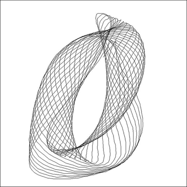
The idea of a harmonograph is not new. It is a mechanical device that started to appear in the mid-nineteenth century and was at the peak of its popularity in the 1890s. It is a mechanical arrangement of pendulums that is used to create complex and detailed patterns by directly drawing them on paper. These things are big, and can be huge, but by using the power of the Raspberry Pi you can make one of a modest size. An example of a pattern produced by this project is shown in Figure 16.1.

Figure 16-1: A harmonograph pattern from the Pendulum Pi.

The Concept

The type of patterns a harmonograph produces are called Lissajous figures, which are much beloved of electronic engineers. In fact the first lab I did as an undergraduate student was to apply two signals from separate signal generators to the X and Y deflection circuits of a cathode ray oscilloscope to obtain them. I sneakily got a third signal generator and applied it to the intensity of the beam, a Z axis modulation, and thoroughly confused the supervising lecturer. However, Lissajous figures are only one simple example of the sort of pattern you can get from a harmonograph. In a harmonograph you can have multiple signals defining each axis, and the slow decay of the amplitude of the swing adds greatly to the complexity of the pattern. So how are you going to computerise this mechanical device? Well the secret lies in being able to measure rapidly the angle of a pendulum. In the last chapter, “Facebook-Enabled Roto-Sketch”, you saw how the rotary shaft encoder could be used to measure the position of a shaft, but the type used there has detents, and requires a relatively large amount of energy to turn. You can get optical shaft encoders with very little friction, but for any great resolution these are horrendously expensive. To the rescue comes a new chip which offers the possibility of a totally friction-free method of measurement – the Hall effect absolute rotary shaft encoder.

The idea is to use four pendulums to create your drawing, and a shaft encoder on each will measure the angle of each pendulum’s swing at any instant of time. Then the Raspberry Pi will plot the information in a window as it comes in, and you will see the picture being plotted in real time. The size of the swing, along with the period of and phase of each pendulum, will alter the picture you produce. You will be able to set the initial swing conditions and alter the length of the pendulums to produce an almost infinite variety of pictures.

The Hall Effect

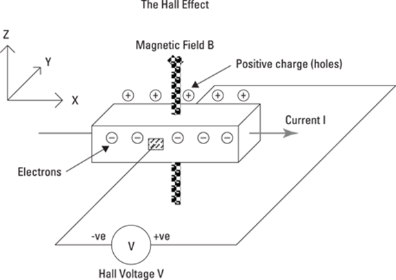
A Hall effect device is one that uses the influence of a magnetic field on a flow of electrons. It was discovered by Edwin Hall in 1879 but has been widely exploited only in the last 30 years or so with the advent of semiconductors. Basically if current is flowing along a conductor, there will be no potential difference on either side of that conductor. However, if a magnetic field is applied upward through the sample perpendicular to the current flow, then the electrons will initially be deflected by the field toward the side of the conductor. They will build up there, with a corresponding number of holes (positive charge) on the other side. This will continue until they build up an electric field that completely balances the force of the magnetic field. Then the electrons can continue traveling in a straight line through the conductor. This is shown in Figure 16.2. So by measuring this voltage across the conductor you can measure the strength of the magnetic field up through the conductor. This is used in all sorts of devices such as contactless switches, contactless current measurement, the electronic compass and angle measurement.

Figure 16-2: How the Hall effect works.

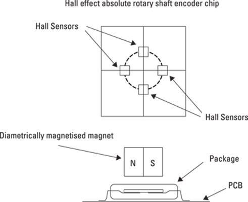
Now an important word in the description “Hall effect absolute rotary shaft encoder” is the word absolute. Many rotary encoders, such as the one used in the last chapter, are only relative encoders – that is, you get a signal only to say something has changed by one notch or increment. With an absolute encoder you get multiple output bits to indicate the actual angle. If you thought optical incremental encoders were expensive, then optical absolute encoders are off the scale of expensive. Fortunately the Hall effect version is relatively cheap. The one I have chosen to use is the AS5040, which will operate over the full 360 degrees and return a 10 bit value. That is, it returns a number between 0 and 1023 for one rotation. This means that it produces a resolution of 0.35 of a degree. It does this by having four Hall effect sensors inside the chip and working out the angle from the relative readings they give. It requires a rather special sort of magnet that is cylindrical and diametrically magnetised. Normally a cylindrical magnet will have a north pole at one end and a south pole at the other. However, when it is diametrically magnetised, there is a north and south pole at each end. Think of this as being two bar magnets glued together and shaped into a cylinder. Fortunately, this type of magnet is easy enough to get.

You have to arrange the magnet on the end of the shaft to be just about 1 mm above the chip. The general arrangement of the chip and magnet are shown in Figure 16.3. This chip is capable of all sorts of outputs, but for this project you are simply going to use the access to the internal registers using the SPI interface pins.

Figure 16-3: The Hall effect sensors in the AS5040.

Enter the Arduino

Now there is one snag with using the Raspberry Pi running Linux with this project, and that is the data from the pendulums is coming out in a constant stream, and, as you know, Linux has a habit of popping out for a cup of tea every now and again. If you were to let this happen, you would have discontinuities in the data, and subsequently, the pattern would look broken up. This is where the Raspberry Pi could do with a little help in reading the data from the sensor, and putting it in a queue or buffer so the Python code can take it out and plot it, without having to worry about when that code is suspended while Linux is doing housekeeping. So here is where the Arduino comes in.

The Arduino is a very popular embedded processor, similar in some respects to the one in the Raspberry Pi. However, it is much, much slower, and has a very small amount of memory – but the Arduino has the advantage of not running an operating system at all. This means that if you program it to do one thing it does it without interruption at a regular rate. What you are going to do is use the Arduino to gather the data from the pendulums, do a bit of processing on it and then send it into the USB serial buffer of the Raspberry Pi. Then this buffer is emptied by the Python program, and the points are plotted on the screen.

The Arduino is programmed in C++, but anyone with any experience in C will be able to write a program for it straight off. It is designed to be used by beginners and nontechnical art users, so it is quite easy to use. It comes with its own integrated development environment (IDE) which is a multiplatform program, and you can run it on the Raspberry Pi, on a laptop or on a desktop machine. There are almost a bewildering variety of Arduinos, but the vanilla one at the time of writing is the Arduino Uno, so that is the one I suggest that you use.

Putting It Together

After you have all the components in place you can start to put them together. The first thing to do is to get the pendulums made. In my version of the harmonograph I have used four pendulums that can be combined in a number of ways to produce the final drawing. In place of the complex arrangement of weights and counterbalances and gimbals used in conventional harmonographs, you just want four simple pendulums of differing lengths. It is the ratio of the pendulum’s periods that gives the fundamental class of the pattern, and integer ratios look best. So with that in mind I calculated some pendulum lengths to produce a fundamental frequency of swing along with twice and three times swing harmonics. These are set out in Table 16.1.

Table 16-1 Length of Pendulum for Various Harmonics

The practical size of the third harmonic pendulum basically governed the size I needed for the fundamental or longest pendulum. You can make the pendulums covering more harmonics if you like, but you will see that they rapidly get quite big. For example, if you want to cover four harmonics, with the shortest pendulum at 100 mm, then the longest pendulum needs to be 3180 mm. The mass of the pendulum does not affect the frequency of swing, but it will affect how long it will swing. In effect it is the damping factor; in other words, the more the mass, the longer it takes for the friction in the bearings to stop the swinging. Getting sufficient mass into short pendulums is tricky; it is easier for longer ones. In fact the equations assume that all the mass of a pendulum is concentrated at the end of the rod or string. What happens in practice with a distributed mass is that the effective length becomes the centre of mass of the pendulum. This means in practice the pendulums have to be slightly longer than the theoretical length.

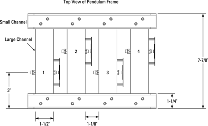
A trip around a national chain of DIY stores brought some rectangular metal tubing and solid bar to my attention, and it looked as if that would do the job for the pendulums. So then I had to design a frame to mount them on. For this I used 1 1/2" by 3/4" by 1/8" and 1 1/14" by 1/2" by 1/8" aluminum channels, referred to as the large channel and small channel, respectively. This has the great advantage that the small channel is a tight fit inside the large one, which makes the design a bit easier. I didn’t find that the DIY stores had this size in stock, so I had to order it online. The idea is to make two U-shaped frames and bolt them together with four lengths of aluminum channel. This is shown in Figures 16-4 and 16-5.

Figure 16-4: The front view of the pendulum frame.

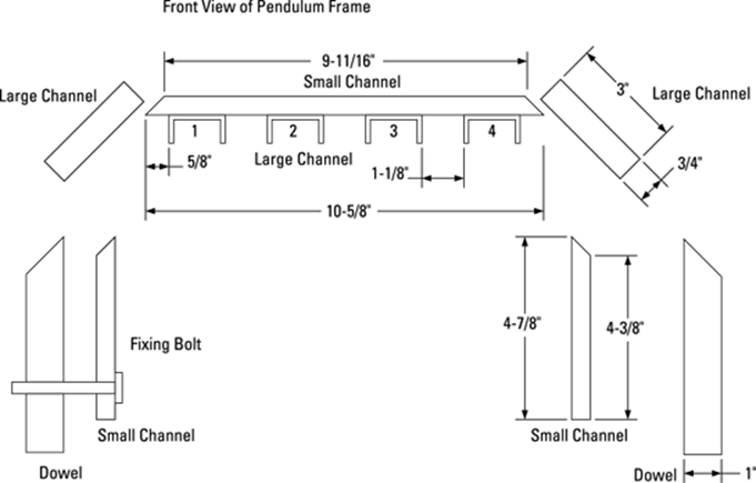
Figure 16-5: The top view of the pendulum frame.

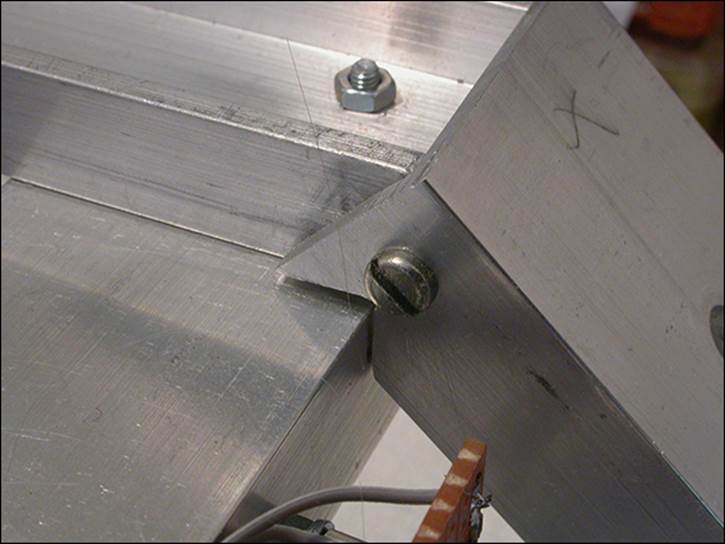
The angled channel fits flush over the far end of the cross channels, but you need to cut out a small notch out of one side of it as shown in Figure 16.6. The fixings for these angled pieces are not nuts and bolts because there is no room for a nut in the cross channel. Therefore, I had to cut a thread into the hole in the cross channel. For the M3 fixings I used, this meant drilling a 2.5 mm hole and running an M3 tap through it. The aluminum is 1/8" thick, so it takes a thread nicely – but remember that it is only aluminum, so don’t tighten it up too much, or you might strip the thread. When cutting thread with a tap, once it is going, always turn it one turn in and then half a turn out. This cuts off the swarf and stops the hole from jamming up. Use a drop of oil when cutting a thread to make the tap last longer. If you are in your local DIY store and ask where the taps are, and are directed to the plumbing section, then find a store that knows what it is selling.

Figure 16-6: The notch needed on one side of each angled channel.

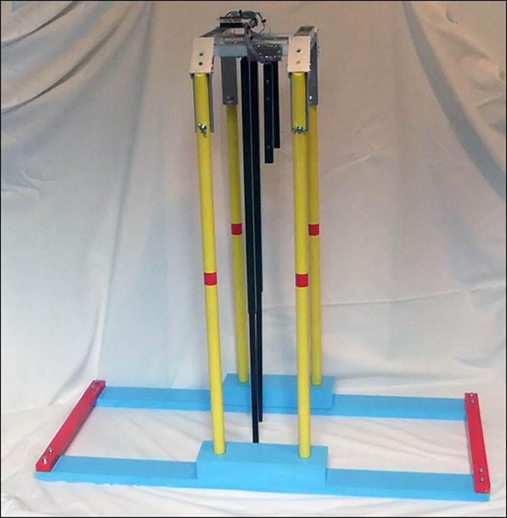
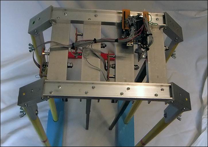
Remember when fixing the aluminum channel together you always need two fixing points per side – one is not enough. The bottom channels of each arm of the frame drop onto four 2' 8" dowel rods, which in turn are set into a floor or bench mounting frame shown in Figure 16.7. I bolted the pieces together with M6 nuts and bolts and fixed a 10" by 3" by 1 1/2" block in the middle of the long side with glue and screws from the underside. I drilled in four 1" holes using a saw drill so that the dowels could be slotted in place. Cut off the dowels at 45 degrees at the top so that they slip under the angled aluminum channel, and a hole through the vertical channel and dowel allows a bolt and wing nut to fasten it into place. Study the finished structure shown in Figure 16.8 to get the idea of what you need to build. The frame on the base is approximately 3' by 1' 4", and contrasting bright colours for the paint can give it more of a fun look.

Figure 16-7: The base frame.

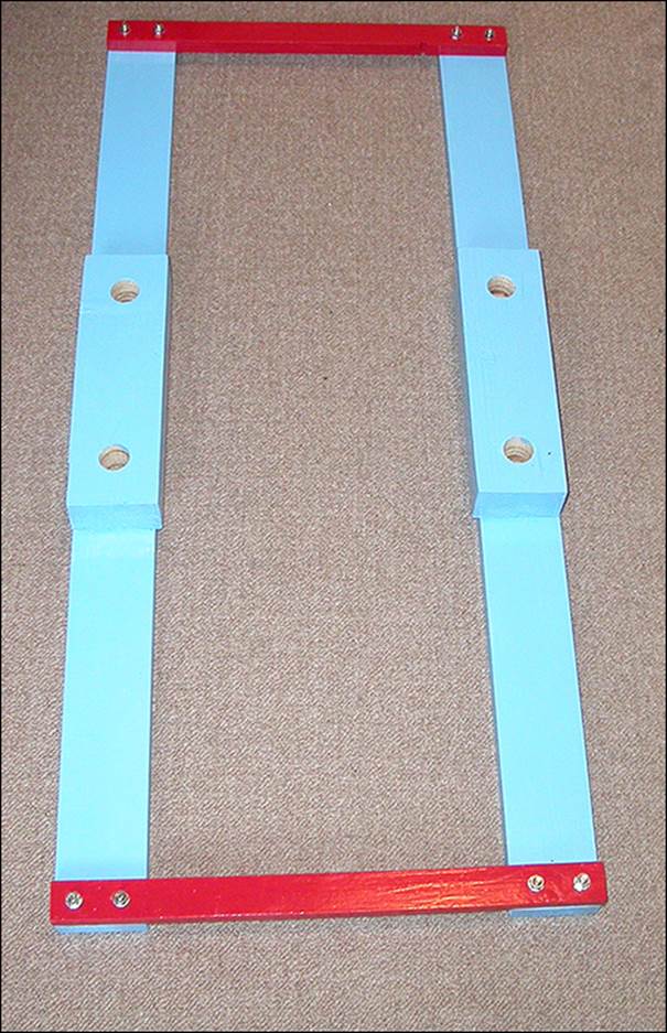
Figure 16-8: The whole pendulum assembly.

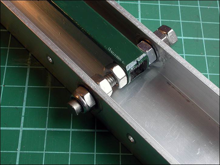
The pendulums themselves are attached to M6 threaded rod, which goes through the sides of the aluminum channel. As shown in Figure 16.9, two lock nuts secure one end; it then passes through a bearing with a nut securing it, and the pendulum is secured to this with another nut. Finally the other end of the channel has a nut on one side of the bearing, with a lock nut on the outside. I drilled out this lock nut’s internal nylon washer and glued in the diametrically magnetised magnet. It is vital that this magnet have its face as square as possible to the rod because this will affect the accuracy of readings that you get.

Figure 16-9: Fixing the pendulum to the threaded rod and channel.

The magnets are extremely powerful and can be prone to damage. Never let them fly together, no matter how tempting it is. This is because they come together with such force that they will shatter and small pieces will chip off them. This can happen the very first time they come together. Another thing is that strong magnets can pick up iron filings in a workshop. You need to remove those to get a uniform magnetic field. I have found the best way is to use blue tack – the sort of putty used for fixing posters to a wall. Use this to mop up a magnet of filings and then throw the piece away. Better still – do not let filings get onto the magnet in the first place.

Smooth Swinging

The bearings I used were the type MR126 sealed, which are quite low cost and are widely used in the construction of 3D printers, inline skates and tools. They have a 6 mm hole for the threaded rod and are 12 mm in diameter. I drilled each side of the channel with a 12 mm drill and used a vice to push the bearings into the hole. This produced a nice interference fit. At first this appeared to work well, but as the threaded rod was tightened up I noticed that there were sections of the rotation that appeared stiff. So in order to exactly align them I filed one hole so that it was slightly larger, allowing a very small amount of slack all around, and then I tightened up the threaded rod and applied epoxy to secure the second bearing (the one not carrying the magnet) in place. In this way I got an exact fit, and the threaded rods would turn on the bearings without any noticeable stiff spots. The pendulum itself is a 12 mm square steel tube, 4" long from the centre of the hole. The area of the tube above the hole needs to be rounded off with a file to prevent it from catching on the top of the aluminum channel. There are two holes at the end of the tube; these should be drilled and tapped with an M3 thread. Although there is not much to thread as the walls of the tube are so thin, this is compensated for by the material being steel; still, overtightening might cause the thread to strip.

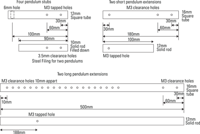
I gave two of the four pendulums, numbers 2 and 4, a solid core of steel by filing down two edges of some 12 mm square steel rod so that it slides inside the tube. Then I marked the position of the tapped holes on the solid rod, drilled out 3.5 mm clearance holes and finally applied some epoxy to hold them in place. You could do that with the other two pendulums as well, but there is little point as these are going to eventually be much longer. The idea is that the basic length of the pendulum is the third harmonic; then there are two sizes of extension rod you can use to get the second harmonic and the fundamental. These are shown in Figure 16.10. The short extensions have a solid square completely contained in the tube, whereas the long extension has the solid rod protruding from the end and the choice of a number of holes along the square tube to attach it, giving you some variability on the length of this largest pendulum. Use positions 1 and 3 for the long pendulum extensions and positions 2 and 4 for the short ones.

Figure 16-10: The pendulum sections.

When sliding the rod up the tube it is a bit hard to spot the tapped hole through the clearance hole. So I painted around the tapped hole with white paint so that it could be easily seen through the clearance hole and lined up correctly.

Electronics

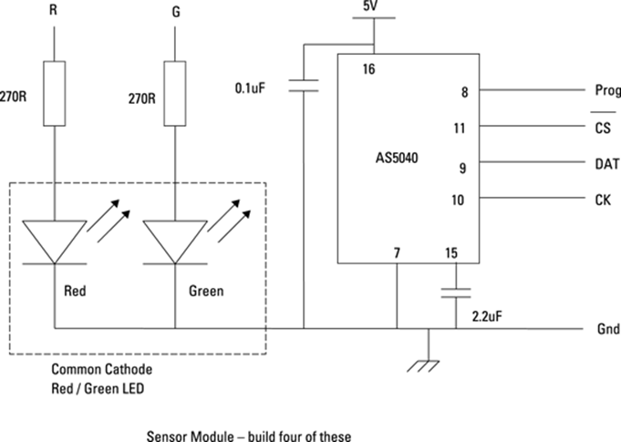
Next, you come to the electronics, which fortunately are not too complex – just the sensor chip, some decoupling capacitors, two resistors and an LED. The AS5040 rotation sensor can be used from either a 3V3 or 5V supply; I used the 5V supply because that gave the correct voltage level of logic signals for the Arduino I used. A schematic of the sensing board is shown in Figure 16.11. You need to build four of these. The capacitors should be of the ceramic type and mounted as close to the chip as possible. The LED is a red/green common cathode, which will allow you to have three colours: red, green and orange. These are used to indicate if the pendulum is being used to gather data and what axis it is controlling.

Figure 16-11: A schematic of one sensor board.

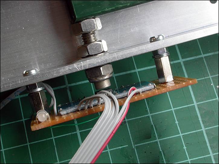
The only difficulty with this circuit is that the AS5040 is in a 16 pin SSOP package, with a 0.65 mm lead pitch. This is impossible to solder directly onto strip board, but fortunately adaptor boards are available quite cheaply. I used a board designed for an SSOP28 chip, and it converts the fine pitch to normal 0.1" pitch used on strip board. (Its full name is an SSOP28 to DIP28 0.65 mm pitch adapter transfer board, and I got it from Hong Kong through eBay.) It covers more chip leads than you need, so just solder it in the centre with three blank connections on each side. This then should be attached to some strip board by soldering solid copper wires through the holes you want connections to. Make sure that the adaptor board is as close as possible to the strip board. Then mount the strip board on the side of each aluminum channel so that the magnet is exactly over the centre of the chip. Separate the pillars by an odd number of strips on the strip board so that the pillar mounting holes are equally spaced from the centre of the bearing/magnet position. To get the distance between the magnet and sensor correct, I used a 10 mm M3 tapped pillar, a nut and two M3 washers and got the spacing between the magnet and chip to be 1 mm. Fortunately there is an electronic way of telling if the magnetic strength is in the correct range; you will see about this later in the chapter when you look at the data that comes from this sensor. The physical arrangement is shown in Figures 16-12 and 16-13.

Figure 16-12: The mounted sensor board showing the chip.

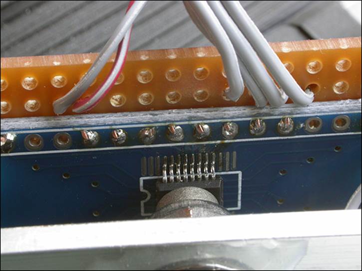
Figure 16-13: The mounting of a sensor board.

Now all that remains is to wire up the sensor modules to the Arduino. The wiring for this is shown in Figure 16.14. The sensors are wired up in a daisy chain configuration with the data from the farthest sensor passing through all the others before it gets to the Arduino. It is common to have multiple sensors wired like this, and it eliminates the need for having a data select line for each chip. I placed a single white LED on the Arduino to indicate if there are any problems with the data from the chips. I drew this module wiring to make the wiring clear; however, in practice I wired it up in a star configuration. That means that the wires are taken directly from each sensor module to the Arduino and not chained, from one sensor board to the next. This ensures that any problems with grounding loops and power distribution are minimised.

Mount the Arduino on pillars on top the pendulum frame as shown in Figure 16.15. Solder the wires to small pieces of copper strip board to which you should solder pin connectors for attaching to the pin headers on the Arduino. Mount the white error LED onto one of these strips close to pin A5. The wiring of the whole thing is shown in Figure 16.16. I used cable ties to make the wiring look neat.

Figure 16-14: A schematic of the sensor modules’ interconnections.

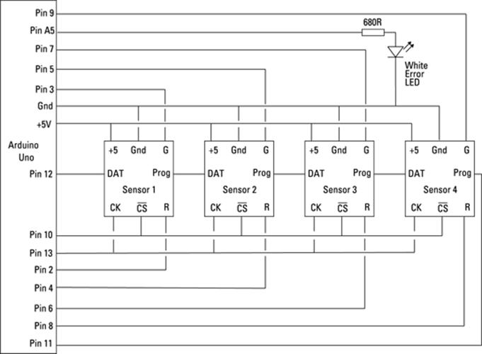
Figure 16-15: The Arduino mounted on top of the frame.

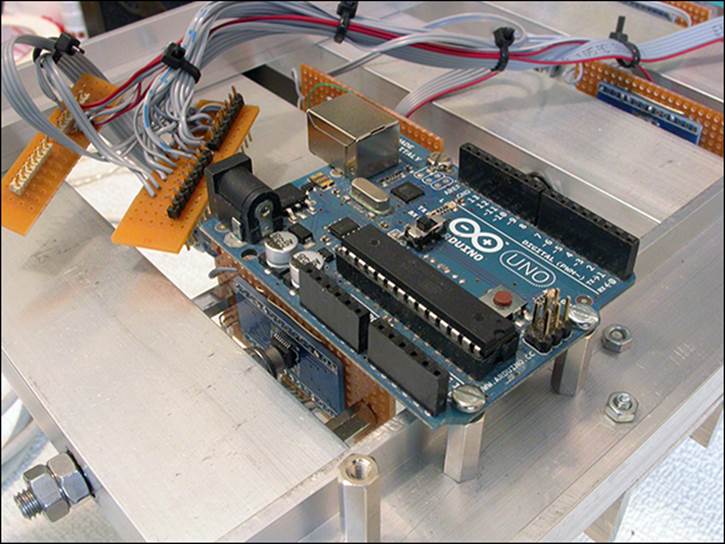
Figure 16-16: The complete system wired up.

Programming the Arduino

Next you have to be able to program the Arduino. To do this you need to use the Arduino IDE. You have a choice of either doing this on your laptop or desktop computer or loading a version into the Raspberry Pi. Using a PC or Mac is much faster than using the Pi, but I have successfully used the Raspberry Pi to program the Arduino. I will show you how to use the Raspberry Pi here.

To install it is simple enough: From a command line just type

$ sudo apt-get update

$ sudo apt-get install arduino

Depending on your Internet access speed this could take 20 minutes or more as you have to download the Java code that supports it. Note that this code might take up more space than you would like; you will be informed of the size before you commit to the download. After it is downloaded start up the desktop and open the File Manager window. Navigate to /usr/bin and double-click the arduino file. A pop-up window will invite you to do various options; click Execute. Plug in your Arduino Uno directly to one of the Raspberry Pi’s USB sockets. I have found that although once programmed the Arduino will work happily through a hub, at the time of writing, the Arduino IDE implementation will not work correctly if it is connected through a hub. Next go to the Tools menu. Choose the Serial Port option and click /dev/ttyACM0. Your Arduino is now connected. Check that the Uno board is selected by clicking Tools → Board.

Now you need to test that everything is working, so type in Listing 16.1.

Listing 16.1 Arduino Blink

// Blink

void setup(){

pinMode(13, OUTPUT);

}

void loop(){

digitalWrite(13, HIGH);

delay(700);

digitalWrite(13, LOW);

delay(700);

}

Now click the right-pointing arrow to upload the blink program into the Arduino. When it has finished uploading the orange LED with a letter L next to it will steadily blink. Click the down-pointing arrow at the top of the IDE window and save your file under the name blink. This will automatically generate a sketchbook folder in your home directory. In the Arduino world the program that runs on an Arduino is known as a sketch.

There are example programs built into the IDE you can look at under File → Examples. After you have the blink sketch in the sketchbook folder you can start the Arduino IDE at any time by double-clicking any of the .ino files in this folder. For now you have only one called blink.ino.

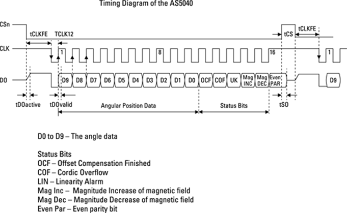
I would encourage you to download and study the data sheet of the AS5040 encoder – it contains a lot more information than you could ever need – but the point is it shows you the full capability of the chip; you are only using a part of its capabilities here. It talks to the outside world using a protocol known as serial protocol interface (SPI), which is a loosely defined protocol that has a lot of subtle differences and variations – so much so that this chip is not quite compatible with the hardware SPI interface of the Arduino, so you will have to write a program to manipulate the SPI lines specifically. This sort of technique is known as bit banging. Figure 16.17 shows the way the interface works. Basically a chip select line is brought low, and then the clock line is made to go up and down – and every time it goes up a new bit of data is placed on the chip’s output. In order for this data to be stable, the Arduino should read the data bit when it places the clock high. As the data appears one bit at a time on the chip’s output the bit banging code must shift it into a variable one bit at a time to make up all 16 bits of the full data. Because you have four of these chips daisy chained together, you must do this four times with a different variable being used to shift the reading each time.

Figure 16-17: The timing diagram for the AS5040 interface.

This is not a book about C or programming the Arduino, so if you are not familiar with them, just treat this section as a black box, the way you treat Python libraries – that is to say you know they work and how to interact with them but you don’t know the details of what they do.

After you install the Arduino IDE and program a flashing LED sketch it is time to test out the sensors and LEDs. It is always good to write something simple to check out the hardware before trying to make it do too much. So type the code in Listing 16.2 into the Arduino IDE.

Listing 16.2 Hardware Test Code

/* Harmonograph reading four rotary encoder

and test out the LEDs

By Mike Cook Feb-April 2013

Bit banging the SPI

*/

// define SPI pins

#define CS_ENC 10

#define CK_ENC 13

#define MISO_ENC 12

#define MOSI_ENC 11

long int time;

byte npRead = 4; // number of detectors to read

float th [] = {0.0, 0.0, 0.0, 0.0 }; // angle reading

int dig1 [] = { 0, 0, 0, 0};

int dig2 [] = { 0, 0, 0, 0};

byte ledRed [] = {2, 4, 6, 8}; // pins controlling red

byte ledGreen [] = {3, 5, 7, 9}; // pins controlling green

int count =1; // LED test pattern

int error = 1; // error LED test count

void setup(){

Serial.begin(9600);

pinMode(CS_ENC, OUTPUT);

digitalWrite(CS_ENC, HIGH);

pinMode(CK_ENC, OUTPUT);

digitalWrite(CK_ENC, HIGH); // set clock high

pinMode(MOSI_ENC, OUTPUT);

digitalWrite(MOSI_ENC, LOW);

pinMode(MISO_ENC, INPUT);

pinMode(A5, OUTPUT);

for(int i=0; i<4; i++){ // set up LEDs

pinMode(ledRed[i], OUTPUT);

digitalWrite(ledRed[i], LOW);

pinMode(ledGreen[i], OUTPUT);

digitalWrite(ledGreen[i], LOW);

}

time = millis() + 2000; // reading every 2 seconds

}

void loop(){

if(millis() > time){ // only take reading every 2 seconds

time = millis() + 1000;

encRead(); // read in all sensors

for(int i =0; i<npRead; i++){ // print them out

Serial.print(th[i]); // angle

Serial.print(" -> ");

Serial.print(dig1[i],HEX); // ready

Serial.print(" -> ");

Serial.println(dig2[i], HEX); // magnetic strength

}

count = count << 1;

if(count > 0xff) count = 1;

upDateLEDs(count);

error++ ;

digitalWrite(A5, error & 1); // flash error LED

Serial.println(" ");

}

}

void upDateLEDs(int n){ // MS nibble red - LS nibble green

ledsOff();

for(int i = 0; i<4; i++){

if( (n & 1) != 0) digitalWrite(ledGreen[i],HIGH);

n = n >> 1;

}

for(int i = 0; i<4; i++){

if( (n & 1) != 0) digitalWrite(ledRed[i],HIGH);

n = n >> 1;

}

}

void ledsOff(){

for(int i=0; i<4; i++){

digitalWrite(ledRed[i], LOW);

digitalWrite(ledGreen[i], LOW);

}

}

void encRead(){ // reads two bytes from each encoder

int hallReading; // to hold 16 bits from sensor

digitalWrite( CS_ENC, LOW); // enable encoders

for(int i = 0; i<npRead; i++){ // read in each sensor

delayMicroseconds(50);

digitalWrite( CK_ENC, LOW); // clock low

delayMicroseconds(50);

for(int i=0;i<16;i++){

// read in all bits for one sensor

hallReading = hallReading << 1;

digitalWrite( CK_ENC, HIGH); // clock high

delayMicroseconds(50);

hallReading = hallReading | digitalRead(MISO_ENC);

digitalWrite( CK_ENC, LOW); // clock low

delayMicroseconds(50);

} // all bits in

digitalWrite( CK_ENC, HIGH); // clock high

delayMicroseconds(50);

th[i] = ((hallReading>> 6) & 0x3ff); // the angle data

dig1[i] = (hallReading & 0x3f) >> 3;

// the magnetic field

dig2[i] = (hallReading & 0x6)>>1;

// ready and error bits

}

digitalWrite( CS_ENC, HIGH); // remove chip enable

}

Now before you run this save it under the name Encoder_read. Then click the tick icon to see if it compiles correctly; any simple mistakes will be highlighted. Correct those and save again. When you can get it to compile without errors click the upload icon to transfer it to the Arduino. This could take up to ten minutes. Only when you have done this should you disconnect the Arduino, plug in the sensor hardware and reconnect the Arduino to the Raspberry Pi.

This sketch reads the sensors and flashes the LEDs in turn at a rate of about two seconds. It prints out the results to the serial port. You can see these results on the serial port terminal program built into the Arduino IDE. Simply click the icon that looks like a magnifying glass in the top-right corner. You will see four groups of numbers, each line being one sensor. The first number is the angle data, followed by the conversion error flags and finally the magnetic indicators. The numbers are separated by an → symbol.

What you are initially looking for is that the second two numbers are 4 and 0, indicating that they are error free, and the first number changes as you move the pendulum. If this is what you see, then it is time to make the adjustments to the pendulums. There is a wraparound point at some place in the rotation where the data goes from 1023 back to zero. You want this point to be outside the permitted swing angle. I adjusted each pendulum’s magnet position by putting the pendulum assembly on its back and just having the short stubs on the pendulums. Then I slackened the nut holding the pendulum to the threaded rod and twisted the rod so that the reading was within 64 of 256 for the pendulum horizontal to one side and within 64 of 768 when moved to the other side. This means that when the pendulums are hanging straight down the reading should be close to 512. The exact value does not matter but write down what it is for each pendulum because you are going to use it in the real sketch so that you get a zero angle reading when the pendulum is hanging straight down.

The Final Arduino Code

Now it is time to program the Arduino for the real job. The Harmo Arduino code is designed to send data to the Raspberry Pi only when it is asked to start. The Pi sends commands to the Arduino that consist of just a single letter. These are Start Sending, Stop Sending and instructions on how to process the pendulum data. So type the code in Listing 16.3 into the Arduino IDE and save it under the name Harmo.

Listing 16.3 The Harmo Arduino Code

/* Harmonograph reading four rotary encoder

By Mike Cook Feb-April 2013

Bit banging the SPI

Sending out to serial port as two 10 bit values split into two

5 bit values with the top two bits used to identify the byte

Serial data flow and configuration control

*/

#define CS_ENC 10

#define CK_ENC 13

#define MISO_ENC 12

#define MOSI_ENC 11

// constants for scaling the output

#define OFFSET 400.0 // centre of the display

#define H_OFFSET 200.0 // half offset

#define RANGE 540.0 // range +/- of co-ordinates

#define H_RANGE 270.0

// half the x range when using two pendulums

long int interval, timeToSample;

float th [] = {0.0, 0.0, 0.0, 0.0 }; // angle reading

// change the line below to your own measurements

int offset[] = {521, 510, 380, 477}; // offsets at zero degrees

int reading[4]; // holding for raw readings

boolean active = false, calabrate = false;

byte np = 2; // number of pendulums to output

byte npRead = 4; // number of detectors to read

byte ledRed [] = {2, 4, 6, 8}; // pins controlling red

byte ledGreen [] = {3, 5, 7, 9}; // pins controlling green

void setup(){

Serial.begin(115200);

pinMode(CS_ENC, OUTPUT);

digitalWrite(CS_ENC, HIGH);

pinMode(CK_ENC, OUTPUT);

digitalWrite(CK_ENC, HIGH); // set clock high

pinMode(MOSI_ENC, OUTPUT);

digitalWrite(MOSI_ENC, LOW);

pinMode(MISO_ENC, INPUT);

interval = 20; // time between samples

timeToSample = millis() + interval;

for(int i = 0; i<4; i++){ // initialise indicator LEDs

pinMode(ledRed[i], OUTPUT);

pinMode(ledGreen[i], OUTPUT);

}

upDateLEDs(np);

delay(100); // allow sensor to power up

pinMode(A5,OUTPUT);

digitalWrite(A5,LOW);

if(calabrate){

encRead(); // get offset

calabrate = false; // calibration done

}

}

void loop(){

if(millis() >= timeToSample && active) {

// send data if we should

digitalWrite(13, HIGH);

timeToSample = millis() + interval;

encRead();

sendData();

digitalWrite(13,LOW);

}

else {

if(Serial.available() != 0) {

// switch on / off sample sending

char rx = Serial.read();

switch (rx) {

case'G': // Go - start sending samples

active = true;

break;

case'S': // Stop - stop sending samples

active = false;

break;

case '2':

// make samples from sensors 1 for X and 3 for Y

upDateLEDs(0x45);

np = 2;

break;

case '3': // samples from sensors 1 & 2 for X and 3 for Y

upDateLEDs(0x47);

np = 3;

break;

case '4':

// samples from sensors 1 & 2 for X and 3 & 4 for Y

upDateLEDs(0xcf);

np = 4;

break;

case '5':

upDateLEDs(0x8a);

np = 5; // make samples from sensors 2 for X and 4 for Y

break;

case '6':

// make samples from sensor 1 for X and 3 & 4 for Y

upDateLEDs(0xCD);

np = 6;

break;

}

}

}

}

void encRead(){ // reads two bytes from each encoder

int hallReading = 0;

digitalWrite( CS_ENC, LOW); // enable encoder

for(int i = 0; i<npRead; i++){

delayMicroseconds(10);

digitalWrite( CK_ENC, LOW); // clock low

delayMicroseconds(10);

hallReading = 0;

for(int i=0;i<16;i++){ // read in all four bits

hallReading = hallReading << 1;

digitalWrite( CK_ENC, HIGH); // clock high

delayMicroseconds(10);

hallReading = hallReading | digitalRead(MISO_ENC);

digitalWrite( CK_ENC, LOW); // clock low

delayMicroseconds(10);

} // all bits in

digitalWrite( CK_ENC, HIGH); // clock high

delayMicroseconds(10);

reading[i] = hallReading;

}

digitalWrite( CS_ENC, HIGH); // remove chip enable

// all data in now process the data

int errorLEDs = 0;

for(int i=0; i<npRead; i++){

th[i] = ((reading[i] >> 6) & 0x3ff) - offset[i];

//angle data

th[i] = th[i] * 0.006135; // convert into radians

if((reading[i] & 0x6) != 0) errorLEDs++;

// shows an error

}

if(errorLEDs != 0) digitalWrite(A5,HIGH);

else digitalWrite(A5,LOW); // drive error LED

}

void upDateLEDs(int n){ // MS nibble red - LS nibble green

ledsOff();

for(int i = 0; i<4; i++){

if( (n & 1) != 0) digitalWrite(ledGreen[i],HIGH);

n = n >> 1;

}

for(int i = 0; i<4; i++){

if( (n & 1) != 0) digitalWrite(ledRed[i],HIGH);

n = n >> 1;

}

}

void ledsOff(){

for(int i=0; i<4; i++){

digitalWrite(ledRed[i], LOW);

digitalWrite(ledGreen[i], LOW);

}

}

void sendData() { // send X Y points to plot

int s1,s2;

byte t;

// pendulums 1 and 3 are short and so have a wider range

switch(np) {

case 2: // from two pendulums

s1 = OFFSET + (RANGE * sin(th[0]));

s2 = OFFSET + (RANGE * sin(th[2]));

break;

case 3: // from three pendulums

s1 = OFFSET + (H_RANGE * sin(th[0])) +

(H_OFFSET * sin(th[1]));

s2 = OFFSET + (RANGE * sin(th[2]));

break;

case 4: // from four pendulums

s1 = OFFSET + (H_RANGE * sin(th[0])) +

(H_OFFSET * sin(th[1]));

s2 = OFFSET + (H_RANGE * sin(th[2])) +

(H_OFFSET * sin(th[3]));

break;

case 5: // from other two pendulums

s1 = OFFSET + (OFFSET * sin(th[1]));

s2 = OFFSET + (OFFSET * sin(th[3]));

case 6: // from three pendulums

s1 = OFFSET + (RANGE * sin(th[0]));

s2 = OFFSET + (H_RANGE * sin(th[2]) +

(H_OFFSET * sin(th[3])));

break;

}

// split up the data into 4 bytes, tag top

// two MS bits and send

t = (s1 >> 5) & 0x1f; // MSB first

Serial.write(t);

t = (s1 & 0x1f) | 0x40; // LSB plus top index bits

Serial.write(t);

t = ((s2 >> 5) & 0x1f)| 0x80; // MSB plus top index bit

Serial.write(t);

t = (s2 & 0x1f) | 0xC0; // LSB plus top index bits

Serial.write(t);

}

The first thing to note is that the line

int offset[] = {521, 510, 380, 477}; // offsets at zero degrees

should be changed to the readings you took with the previous sketch when the pendulums were hanging down. It is impossible that you will have the same readings here for your construction.

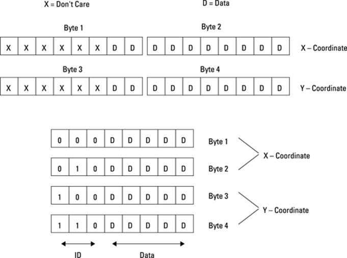
One important thing to note is the way the data is sent to the Raspberry Pi. In order to minimise the number of bytes sent, you send only the X and Y coordinates that need to be plotted. However, you can’t just send the bytes because you then have no way of knowing which was which at the receiving end. If one was missed, then the whole thing would be out of sequence, and the data would be corrupted. There are two ways around this problem: The first is to send data in packets – send the data and add a header to it. The header should be a unique value that does not appear in the data. The receiving side keeps fishing bytes out of its buffer until it sees this header byte; then it has a good chance of knowing that the next few bytes are in the order they are sent. This is fine especially for larger amounts of data, but you have to ensure a unique value for the start of packet indicator, and that often means restricting the data to something like a string representation, which is inefficient. Here, the approach I have used is to tag each individual byte, which works because you are trying to send two 10-bit data values and there are plenty of spare bits if you divide the data up correctly. Figure 16.18 shows what I have done. Basically each coordinate is split up into two 5-bit fields, and the top two bits of each field have a unique bit pattern to identify them. Therefore the receiving side can identify if the bits come in in the right order and verify that none have been dropped. This was important, especially during development, because initially the Raspberry Pi’s buffer was filling up to overflowing and data was being lost. Therefore I knew I had to do something to alleviate the problem; more on that when you see the Python code in the section “Programming the Pi”.

Figure 16-18: Splitting up the data to tag each byte.

The other main point is the code that looks at the serial port to see if the Raspberry Pi has sent any data back. You will see that all that happens is that variables are set, but these variables affect the program flow later on, specifically in the sendData() function. This function converts the angles you measure from each pendulum into the distance to plot on the screen. Using the simple sin rule of geometry shown in Figure 16.19, you can calculate the distance from the centre of the swing.

Figure 16-19: Generating a displacement from an angle.

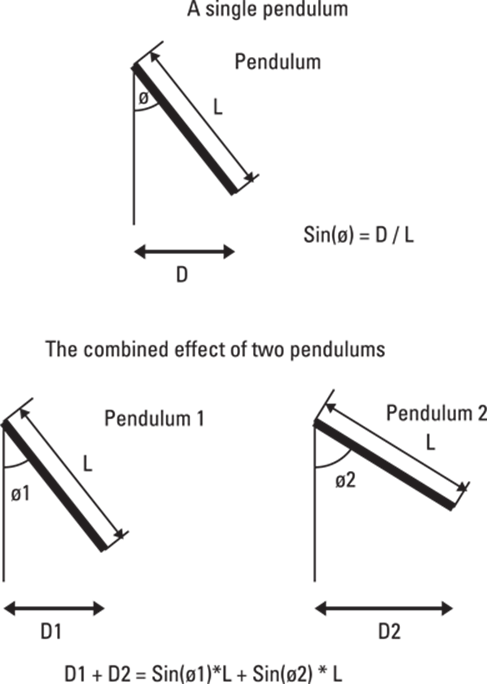
The actual length of the pendulum is substituted by a value of half the number of pixels you want to cover, and when you have two pendulums you use half that value and add them up. In the sketch you will see that this is not quite the case with the values of the constant RANGE; this is because the large pendulums do not swing as much as the small ones, so there is a bit of an amplification factor to make a slightly bigger display. When two pendulums are used, the displacement distance at any time is simply the two pendulum readings added together. As they swing back and forth you need to add a fixed offset so that the swing will be in the centre of the window when you plot it on the Raspberry Pi. You will see in the sendData() function the angle data from each pendulum can be combined in a number of different ways depending on what commands have been received. Then finally the data is split up, tagged and sent out of the serial port to the Raspberry Pi.

Programming the Pi

Finally you have come to the point where you want to take the data streaming in from the pendulums and plot them onto the screen to see what patterns they make. The first thing a program has to do is to establish communication with the Arduino. When you plug an Arduino into the USB port it can potentially appear on one of two ports, so you have to try both of them. You want to send the data as fast as possible, so use the Arduino’s top speed of 115200 baud. Then you have to open a Pygame window and command the Arduino to start sending data by sending it the letter Gfor “go”, down the serial port. The full listing of the Python program to do this is shown in Listing 16.4.

Listing 16.4 The Pendulum Pi Plotting Program

import piface.pfio as pfio # piface library

#!/usr/bin/env python

"""

Harmonograph plotter

Data comes from pendulums attached to an arduino and feeding

into the Pi through the USB serial port

version 2 with reduced byte transfer count

"""

import time # for delays

import os, pygame, sys

from pygame.locals import *

import serial

try:

ser = serial.Serial('/dev/ttyACM0',115200, timeout=2)

except:

ser = serial.Serial('/dev/ttyACM1',115200, timeout=2)

pygame.init() # initialise graphics interface

os.environ['SDL_VIDEO_WINDOW_POS'] = 'center'

pygame.display.set_caption("Harmonograph")

screen = pygame.display.set_mode([800,800],0,32)

background = pygame.Surface((800,800))

cBackground =(255,255,255)

background.fill(cBackground) # make background colour

col = (0,0,0) # drawing colour

reading = [0, 0, 0, 0]

lastX = 0

lastY = 0

picture = 1 # picture number

nextTime = time.time()

timeInc = 0.2 # update screen every half a second

fileName = "harmo"

running = False

def main():

openPort()

getData()

drawData() # to get the starting positions

blank_screen()

while True :

checkForQuit()

getData()

drawData()

def drawData():

global readings, nextTime, lastX, lastY

x = reading[0]

y = reading[1]

pygame.draw.line(screen,col,(lastX,lastY),(x,y),1)

lastX = x

lastY = y

# see if it is time to update the screen

if time.time() > nextTime :

pygame.display.update()

nextTime = time.time() + timeInc

def openPort():

global running

ser.flushInput()

# tell the arduino to start sending

running = True

ser.write('3')

ser.write('G')

def checkInput(b):

# see if the bytes have been received in the correct order

correct = True

for i in range(0,4):

#print i," - " # ,hex(ord(b[i]))

if (ord(b[i]) >> 6) != i :

correct = False

return correct

def getData():

global reading, running

if running :

a = ser.read(4)

if checkInput(a) :

reading[0] = ((ord(a[0]) & 0x1f)<< 5) |

(ord(a[1]) &0x1f)

reading[1] = ((ord(a[2]) & 0x1f)<<5) |

(ord(a[3]) &0x1f)

#print reading[0]," - ",reading[1]

else:

correct = False

while correct == False : # resynchronise

print "lost sync ",ser.inWaiting()

b = ser.read(1)

t = a[1] + a[2] + a[3] + b[0]

a = t

correct = checkInput(a)

def blank_screen():

screen.fill((255,255,255)) # blank screen

pygame.display.update()

def terminate(): # close down the program

print ("Closing down please wait")

# tell the arduino to stop sending

ser.write('S')

ser.close()

pygame.quit()

sys.exit()

def checkForQuit():

global col, picture, fileName, running

event = pygame.event.poll()

if event.type == pygame.QUIT :

terminate()

elif event.type == pygame.KEYDOWN :

# get a key and do something

if event.key == pygame.K_ESCAPE :

terminate()

if event.key == K_SPACE or event.key == K_DELETE:

blank_screen()

if event.key == K_r :

col = (255, 0, 0)

if event.key == K_g :

col = (0, 255, 0)

if event.key == K_b :

col = (0, 0, 255)

if event.key == K_y :

col = (255, 255, 0)

if event.key == K_m :

col = (255, 0, 255)

if event.key == K_c :

col = (0, 255, 255)

if event.key == K_w :

col = (255, 255, 255)

if event.key == K_k :

col = (0, 0, 0)

if event.key == K_s : # see the size of the buffer

print ser.inWaiting()

if event.key == K_2 :

ser.write('2') # data from two pendulums

if event.key == K_3 :

ser.write('3') # data from three pendulums

if event.key == K_4 :

ser.write('4') # data from four pendulums

if event.key == K_5 :

ser.write('5') # data from alternate two pendulums

if event.key == K_6 :

ser.write('6')

# data from alternate three pendulums

if event.key == K_h :

ser.write('S') # stop arduino from sending

running = False

if event.key == K_j :

ser.write('G') # start arduino sending

running = True

if event.key == K_HOME :

ser.write('S') # stop arduino from sending

print "save sketch to file"

if picture == 1 : # first time to save this session

fileName = raw_input("Enter file name

for this session ")

try:

pygame.image.save(screen,'harmo/'+

fileName+str(picture)+'.png')

except:

os.system('mkdir harmo')

pygame.image.save(screen,'harmo/'+

fileName+str(picture)+'.png')

print "saving sketch as ",'harmo/'+

fileName+str(picture)+'.png'

picture +=1;

ser.write('G') # start arduino sending

if __name__ == '__main__':

main()

If you get an error at the line

import serial

Then you will have to install it by typing

sudo apt-get python-serial

The main function is quite simple: It opens the serial port and then gets one point of data, plots it and wipes the screen. This primes the last coordinate positions so that the drawing starts at the current point. Then there is a simple infinite loop that checks for any quit or keyboard inputs, and then gets another pair of points and plots them. The getData() function simply reads four bytes from the serial port, and the checkInput() function is called as part of an if statement. This returns true or false depending whether the input bytes have the correct tag bits on them. If they are okay, the bytes are unpacked into a reading variable; if not then a message is printed out, and bytes are read in one at a time in an attempt to resynchronise the data stream.

Drawing the data on the screen is quite simple and handled by the drawData() function. A line is drawn between this new pair of points and the last set. Now at this point you might expect to update the screen. However, when I tried this it took too long, and the data backed up in the buffer leading it to overflow and thus fail. So I came up with the compromise that the actual screen would only be updated every 0.2 of a second. This is done by using the timer module to see if it is time to update the screen. This results in a slightly jerky drawing, but it is not too disturbing to look at. As a result, in normal circumstances, the buffer is nearly always empty. However, when the operating system times out the program, the buffer is big enough to cope, and the display is not disturbed. You can see the display very rapidly catch up when the program returns.

The other main part of the program is the checkForQuit() function. This checks for the Esc key or the window close click as normal, but it also checks to see if any keyboard key has been pressed. These are used for various functions, as summarised in Table 16.2.

Table 16-2 Keyboard Functions

Using the Pendulum Pi

To finish off, here are a few notes on using the Pendulum Pi. To get a feel of what is going on, start off with a simple two pendulum by pressing the 2 key. Now swing the two long pendulums at positions 1 and 3 exactly together or as we say, “in phase”; you will see a diagonal line at about 45 degrees being drawn. Now make them swing exactly opposed to each other – that is, 180 degrees apart – and you will see the same diagonal line but drawn in the opposite direction. Finally, get them at 90 degrees apart, let one go and release the second when the first is at the bottom of its swing. What you should then see is a circle. Of course you will not get it exactly spot on so what you will actually see is an elongated ellipse instead of a straight line and a fat ellipse instead of a circle. You might want to try some fine adjustment on the pendulums’ length to get them to swing exactly at the same rate. As the two drift out of phase you will see the same shapes being traced slightly shifted. This is where it starts getting interesting as pleasing patterns are built up.

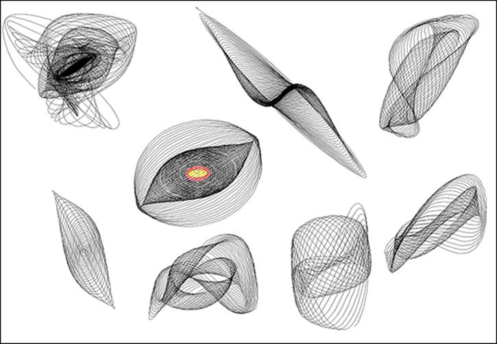
Also as the swing decays, the excursions will get smaller, and the pattern being drawn will slowly get smaller. This also adds interest to the pictures drawn. Now switch to a three pendulum setup, and see how the second pendulum modifies the swing plotted. I have found it best if you release the pendulums from a height rather than pushing them. Also, don’t just swing them the maximum amount they will go; often less is more. You will also find some energy is transferring from one pendulum to another, which also adds to the variety of patterns you can get. There are many patterns you can generate from just one setup. Figure 16.20 shows some of the patterns I have managed to generate in a few sessions. To save a picture, press the Home key on the keyboard. You will then be asked for a session name in the Python console. Odds are you will have to click the console window to give it focus while you type in the base name. After you have done this for the first time any further screen saves use the same filename with an increasing number tacked on. These are stored in a folder called harmo, so make sure that you create one first.

Figure 16-20: Some of the patterns generated with this project.

Over to You

I think the best patterns are achieved when the long and short pendulums are an integer harmonic of each other, so you might want to change the way the long pendulum’s length is adjusted to get a finer degree of control over it. You could write some software to measure the period of the pendulum to allow you to adjust the period even more accurately.

You could make the frame higher so that you could use longer pendulums and get higher ratios of swing. A pendulum of just over three meters might be pushing how much space you have in a domestic environment, however.

You could add the automatic Facebook posting of the pictures as shown in the last chapter.

One enhancement that would involve changing the Arduino software is to use one of the pendulums to send information that changes the colour of the trace in a gradual way. That would produce smoothly changing multicolour traces – although you might want to try that idea purely in the Python software based on the number of samples received. You can explore the difference between RGB colour space and HSV colour space in the colour changing.

One radical change you could do is to generate the swings purely in software using the same algorithm, either in the Arduino or the Raspberry Pi. This will allow you to produce patterns with a high swing ratio that otherwise would require very long pendulums. However, you will have to model the swing decay, and you won’t get the energy transfer effects – so in my opinion, it is not nearly as much fun as swinging them and seeing what you get.