Programming 3D Applications with HTML5 and WebGL (2013)

Part I. Foundations

Chapter 5. 3D Animation

Animation means making changes to the image on the screen over time. With animation, an otherwise static 3D scene comes to life. While there are many techniques for animating, and many ways to model the problem conceptually, at the end of the day, animation is all about one thing: making the pixels move.

WebGL doesn’t have built-in animation capability per se. However, the power and speed of the API allow us to render amazing graphics and change them at up to 60 frames per second, providing us with several options for animating 3D content. Combined with improvements to the runtime architecture of modern browsers, this enables animations that blend seamlessly with the other elements on the page, without tearing or other unwanted artifacts.

Animation can be used to change anything in a WebGL scene: transforms, geometry, textures, materials, lights, and cameras. Objects can move, rotate, and scale, or follow paths; geometry can bend, twist, and change into other shapes; textures can be moved, scaled, rotated, and scrolled, and have their pixels modified every frame; material colors, specular highlights, transparency values, and more can change over time; lights can blink, move, and change color; and cameras can be moved and rotated to create cinematic effects. The possibilities are essentially limitless.

In this chapter, we will look at a variety of animation techniques, and the tools and libraries to implement them. These techniques are grounded in years of film and video game industry practice, backed by rigorous mathematics. Animation with WebGL is an evolving area, so our exploration involves cobbling together various solutions. Three.js comes with animation utilities that handle certain situations well. We will also look at another open source library, Tween.js. Tween.js is a small, easy-to-use library for creating simple transitions. But these are far from complete packages. If your application is sufficiently complex, you may need to create your own animation engine.

Animating WebGL content involves employing one or more of the following concepts, which will be covered in detail in this chapter:

§ Using requestAnimationFrame() to drive the run loop.

§ Programmatically updating properties of visual objects each time through the run loop. This is good for creating simple animations, such as spinning an object about a single axis. This technique can also be useful when an object’s position, orientation, or other property is best expressed as a function of a variable such as time. Overall, this is the simplest animation technique to implement, but it is limited to very specific use cases.

§ Using tweens to transition properties smoothly from one value to another. Tweens are perfect for simple, one-shot effects (e.g., moving an object from one position to another along a straight path).

§ Using key frames, where data structures represent individual values along a timeline, and an engine calculates (interpolates) intermediate values to produce a smooth result. Key frames work well for basic animation of translation, rotation, and scale, and simple properties such as material colors. Unlike tweens, which support a single transition from one value to another, key frames allow us to create a series of transitions within one animation.

§ Animating objects along paths—user-generated curves and line segments—to create complex and organic-looking motion based on formulas or preauthored path data.

§ Using morph targets to deform geometry by blending among a set of distinct shapes. This is an excellent technique for facial expressions and for very simple character animation.

§ Using skinning to deform geometry based on animating an underlying skeleton. This is the preferred way to animate characters and other complex shapes.

§ Using shaders to deform vertices and/or change pixel values over time. Sometimes, a desired animated effect is best calculated on a per-vertex or per-pixel basis, suggesting the use of GLSL to implement it. Shaders can also be used to accelerate the performance of the other techniques—in particular, morphs and skinning, which can be computationally expensive if done on the CPU.

Often an application will make use of more than one, or sometimes all, of these approaches. There are no hard and fast rules about which techniques apply in which situations, though some are better suited for implementing particular effects. Often the choice of technique is driven by production concerns; for example, if you don’t have a needed artist on staff, it may be easier to have a programmer generate the animations in code. Other times, it may simply come down to personal preference. 3D animation is equal parts art and science, a mix of production and engineering.

Driving Animation with requestAnimationFrame()

In previous chapters we saw how to power our application’s run loop using requestAnimationFrame(), a relatively recent arrival to web browser APIs.

requestAnimationFrame() was designed to allow web applications to provide consistent, reliable presentation of visual content driven by JavaScript code. The content might be changing the page DOM, adjusting layouts, modifying styles using CSS, or creating arbitrary graphics with one of the drawing APIs such as WebGL and Canvas. The feature was first introduced in Firefox version 4 and eventually adopted by all the other browsers. Robert O’Callahan of Mozilla was looking for a way to ensure that animations handled by the browser for built-in features like CSS Transitions and SVG could be synchronized with user code written in JavaScript.

Historically, web applications used timers to animate page content, via either setTimeout() or setInterval(). As applications began to incorporate more complex animations and interactivity, it became clear that this approach suffered from several key problems:

§ The timer functions call callbacks at a specific interval (or as close to it as possible), regardless of whether it is a good time to draw or not.

§ JavaScript executed in a timer callback has no reliable way to synchronize with the timing of other browser-generated animation on the page (e.g., SVG or CSS Transitions).

§ Timers execute regardless of whether a page or tab is visible or the browser window has been minimized, potentially resulting in wasted drawing calls.

§ JavaScript application code has no idea of the display’s refresh rate and so has to make an arbitrary choice for the interval value: make it 1/24 of a second, and you deprive the user of resolution on a 60 Hz display; make it 1/60 of a second and on slow-refresh displays, you waste CPU cycles drawing content that is never seen.

requestAnimationFrame() was designed to solve all of the preceding problems. Recalling examples from previous chapters, our run loop takes a form similar to the following:

function run() {

// Request the next animation frame

requestAnimationFrame(run);

// Run animations

animate();

// Render the scene

renderer.render( scene, camera );

Note the absence of a time value in the call to requestAnimationFrame(). We are not asking the browser to call our animation and drawing code at any specific time or interval; rather, we are asking it to call it when it is ready to present the page again. This is a key distinction. With this scheme in place, the browser can call user drawing code during its internal repaint cycle. This has several benefits. First, the browser can do this as frequently—or equally important, as infrequently—as needed. When the browser has sufficient idle cycles, it can try to ensure the highest frame rate possible to match the display refresh rate. Conversely, if a page or tab is hidden, or the entire browser is minimized, it can throttle the amount of times it calls such callbacks, optimizing use of the computer or device’s resources. Second, the browser can invoke batch user drawing, which ultimately results in fewer repaints of the screen, also a resource saver. Third, any user drawing code executed from requestAnimationFrame() will be blended, or composited, with all other drawing calls, including internal ones. The net result of all this is smoother, faster, more efficient page drawing and animation.

Using requestAnimationFrame() in Your Application

Like many recent developments in the HTML5 suite of features, requestAnimationFrame() is not necessarily supported in all versions of all browsers—though that is rapidly changing. Also, given its evolution from an experimental feature in one browser through to W3C recommendations, the function has been implemented with different, prefixed names in each of the browsers. Thankfully, we can make use of a great polyfill created by Paul Irish at Google. The code for it, listed in Example 5-1, can be found in the book example filelibs/requestAnimationFrame/RequestAnimationFrame.js. It attempts to find the correctly named version of the function for the current browser or, failing that, falls back to setTimeout(), going for it with a 60 frames-per-second interval.

Example 5-1. RequestAnimationFrame polyfill by Paul Irish

/**

* Provides requestAnimationFrame in a cross browser way.

* http://paulirish.com/2011/requestanimationframe-for-smart-animating/

*/

if ( !window.requestAnimationFrame ) {

window.requestAnimationFrame = ( function() {

return window.webkitRequestAnimationFrame ||

window.mozRequestAnimationFrame ||

window.oRequestAnimationFrame ||

window.msRequestAnimationFrame ||

function( /* function FrameRequestCallback */ callback,

/* DOMElement Element */ element ) {

window.setTimeout( callback, 1000 / 60 );

};

} )();

}

NOTE

For those not familiar with the term, a polyfill is code (usually JavaScript) that provides facilities not built into a web browser. Polyfills are routinely used with older browser versions that do not support new or experimental features. The term was coined by UK-based engineer Remy Sharp. For more on the background and etymology of the polyfill, consult Sharp’s blog posting.

One key to successful use of requestAnimationFrame() is to make sure you request the next frame before calling any other user code, as was done in the run loop fragment shown earlier. This is important for dealing with exceptions. If you are driving your entire 3D application from the animation callback, and code somewhere generates an exception before requesting the next frame, your application is dead. However, if you request the next frame before doing anything else, at least you are guaranteed to continue running. This allows parts of your application to function and repaint elements, even if something is wrong elsewhere.

requestAnimationFrame() and Performance

While requestAnimationFrame() is a boon for animation performance, it comes with a certain responsibility. If the browser is calling your callback every 60th of a second, the onus is on you to write callbacks that take 16 milliseconds or less. If you don’t, your application may appear unresponsive to the user. Because 16 milliseconds is not a lot of time, you must take care to do the minimum amount of work required to make the necessary drawing changes and no more. Industrial-strength 3D applications might consider using timers, workers, and other animation techniques like CSS Transforms and Transitions in conjunction with requestAnimationFrame() to deliver the most responsive, powerful, resource-efficient experiences possible.

NOTE

requestAnimationFrame() is arguably one of the most important features introduced for HTML5. This section merely scratched the surface on the topic. There are several excellent online resources for learning more about it. Do a web search on the name and you will discover a trove of articles, backgrounders, how-tos, tips and tricks, and explanations of what is under the hood.

Frame-Based Versus Time-Based Animation

Early computer animation systems emulated predecessor film animation techniques by presenting a succession of still images on the display, or, in vector-based graphics, a series of vector-based images generated by the program. Each such image is known as a frame. Historically, film was shot and played back at a rate of 24 images every second, known as a frame rate of 24 frames per second (fps). This speed was adequate for large projection screens in low light settings. However, in the world of computer-generated animation and 3D games, our senses are actually able to perceive and appreciate changes that occur at higher frame rates, upward of 30 and up to 60 or more fps. Despite this, many animation systems, such as Adobe Flash, originally adopted the 24 fps convention due to its familiarity for traditional animators. These days, the frame rates have changed—Flash supports 60 fps if the developer requests it—but the concept of discrete frames remains. This technique of organizing animation into a series of discrete frames is known as frame-based animation.

Frame-based animation has one serious drawback: by tying it to a specific frame rate, the animator has ensured that animation will never be able to be presented at a higher frame rate, even if the computer can support it. This was not an issue for film, where the hardware was fairly uniform throughout the industry. However, in computer animation, performance can vary wildly from device to device. If you create your animations at 24 fps, but your computer can refresh the screen at 60 Hz, you effectively deprive the user of additional detail and smoothness during playback.

A different technique, known as time-based animation, solves this problem. In time-based animation, a series of vector graphics images is connected to particular points in time, not specific frames in a sequence with known frame rates. In this way, the computer can present those images, and the interpolated frames between them, as frequently as possible and deliver the best images and smoothest transitions. In the examples in the previous chapters, we used time-based animation. Each time through the run loop, the animate() function calculated a time delta between the current and previous frame and used that to compute an angular rotation. All of the examples developed for this and subsequent chapters use time-based animation. So, even though the word frame is right in the name requestAnimationFrame(), rest assured that it can be used equally well for time-based animations.

Animating by Programmatically Updating Properties

By far, the simplest way to get started animating a WebGL scene is to write code that updates an object’s properties each time through the run loop. We have seen examples of this already in previous chapters. To rotate the Three.js cube in Chapter 3, we simply updated the cube’srotation.y property—that is, the angle of its rotation about the y-axis, each frame. Here is the code again:

var duration = 5000; // ms

var currentTime = Date.now();

function animate() {

var now = Date.now();

var deltat = now - currentTime;

currentTime = now;

var fract = deltat / duration;

var angle = Math.PI * 2 * fract;

cube.rotation.y += angle;

}

The variables duration, currentTime, now, and deltat are used to compute a time-based animation value for the rotation. In this example, we want a full rotation about the y-axis over the course of five seconds. The computed angle is a fraction of one complete rotation, the amount that must be added to the cube’s current rotation.y property. Recall that rotations are represented in Three.js as radians, the distance around a unit circle; that is, Math.PI * 2 is equal to a full (360 degree) rotation.

This concept can be applied to animate anything in a scene: position, rotation, scale, material colors and transparency, and so on. Moreover, it is completely general: by using JavaScript code to update properties, we can apply arbitrary computation. Animations can be driven by mathematical formulae, Boolean logic, statistical values, data streams, real-time sensor input, and so on. So this is a great technique for scientific illustration and data visualization: depicting solar systems, physical processes, and natural phenomena; or presenting time series information, statistical analyses, geographic data, website traffic, and other dynamic, database-driven information. It is also excellent for creating really lively and entertaining applications like music visualizers.

Figure 5-1 depicts the wild world of Ellie Goulding’s Lights, a WebGL music visualization developed by UK-based interactive agency Hello Enjoy. This piece has been around for a while, but it still packs a punch. Glowing globes blink on and off, comet trails wind a curvy path through the scene, colored balls fade in and out and change color, spotlights twirl madly, and teardrop-shaped balloons blossom out of the multicolored, undulating terrain—all in time to the music of the hit song. This is eye candy at its best, with all effects being generated programmatically.

Example 5-2 shows a portion of the code that animates the visuals. The application’s update() method is called each time through the run loop. It in turn calls update() on all the objects in the scene. The following excerpt is from LIGHTS.StarManager.update(), which animates the background stars. The stars are rendered as Three.js particles belonging to a THREE.ParticleSystem object. The lines highlighted in bold show how the RGB color for each star is updated based on elapsed time, a decay factor, and the mod operator (%) to create a blink effect.

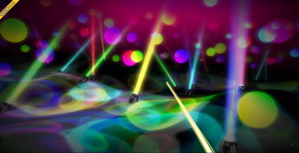
Figure 5-1. Ellie Goulding’s Lights: A music visualizer built with programmatic animation; image courtesy Hello Enjoy, Inc.

Example 5-2. Animating to the beat: Code fragment from Ellie Goulding’s Lights

update: function() {

var stars = this.stars,

deltaTime = LIGHTS.deltaTime,

star, brightness, i, il;

for( i = 0, il = stars.length; i < il; i++ ) {

star = this.stars[ i ];

star.life += deltaTime;

brightness = (star.life * 2) % 2;

if( brightness > 1 )

brightness = 1 - (brightness - 1);

star.color.r =

star.color.g =

star.color.b = (Math.sin( brightness * rad90 - rad90 ) + 1) * 4;

}

this.particles.__dirtyColors = true;

},

As flexible and powerful as programmatic animation is, it has its limitations. It requires handcoding for each effect; as a consequence, it’s hard to scale up to animate many different kinds of objects. It also tends to be more verbose than other data-driven methods such as tweening and key frames, which we will cover shortly. Finally, it puts the programmer at the center of the action, instead of the artist, who may be much better suited to creating the desired visual effect. Still, programmatic animation is an excellent way to quickly and easily add some life to a scene, and the effects can be truly stunning, as in the case of Ellie Goulding’s Lights.

Animating Transitions Using Tweens

Many animation effects are better represented as data structures, rather than values that are programmatically generated each time through the run loop. The application supplies a set of values and a time series, and a general-purpose engine calculates the per-frame values used to update properties. One such data-driven approach is known as tweening.

Tweening is the process of generating values that lie between a pair of other values. With tweening, the animator supplies only the values at the beginning and end points of the animation, and the engine calculates the intermediate values (tweens) for the intervening times. Tweening is perfect for simple one-time transitions from one state to another, such as moving an object in reaction to a mouse click.

Interpolation

Tweening is accomplished through a mathematical technique called interpolation. Interpolation refers to the generation of a value that lies between two values, based on a scalar input such as a time or fraction value. Interpolation is illustrated in Figure 5-2. For any values A and B, and a fraction u between 0 and 1, the interpolated value P can be calculated by the formula A + u * (B − A). For the example depicted in Figure 5-2, we can see the interpolated value P(u) = 0.4. This is the simplest form of interpolation, known as linear interpolation because the mathematical function used to calculate the result could be graphed with a straight line. Other, more complex interpolation functions, such as splines (a type of curve) and polynomials, are also commonly used in animation systems. We will look at spline-based animation shortly.

Interpolation is used to calculate tweens of 3D positions, rotations, colors, scalar values (such as transparency), and more. With a multicomponent value such as a 3D vector, a linearly interpolated tween simply interpolates each component piecewise. For example, the interpolated value P at u= 0.5 for the 3D vector AB from (0, 0, 0) to (1, 2, 3) would be (0.5, 1, 1.5).

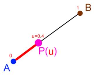
Figure 5-2. Linear interpolation; reproduced with permission

The Tween.js Library

It is pretty straightforward to implement simple tweening on your own. However, if you want to have nonlinear interpolation functions, and other bells and whistles such as ease in/ease out (where the animation appears to accelerate to its main speed and decelerate out of it), then the problem becomes more complex. Rather than build your own tweening system, you may want to use an existing library. Tween.js is a popular open source tweening utility created by Soledad Penadés. It has been used in conjunction with Three.js on popular WebGL projects, including RO.ME, the WebGL Globe, and Mine3D, a web version of the classic single-player game Minesweeper.

The example in the file Chapter 5/tweenjstweens.html contains a sandbox for testing out various Tween.js options. See Figure 5-3 for a screenshot. The sandbox uses Tween.js to apply various transitions to a textured cube: position, rotation, material color, and opacity. There are sliders for adjusting the tween duration and delay time (time before the tween starts), checkboxes to enable and disable the specific tweens, and an option to loop the tween (repeat it continuously). There is also an option to control easing functions, but we will talk about that in the next section. Play with the different options to see how they modify the effect.

Tween.js is very easy to work with. The syntax is simple, and thanks to the polymorphism of JavaScript, we can target any property using the exact same method calls. It also uses chained method syntax similar to jQuery, allowing for a very concise expression. Let’s have a look. Example 5-3shows a portion of the function playAnimations(), called to trigger the tweens each time a property is changed.

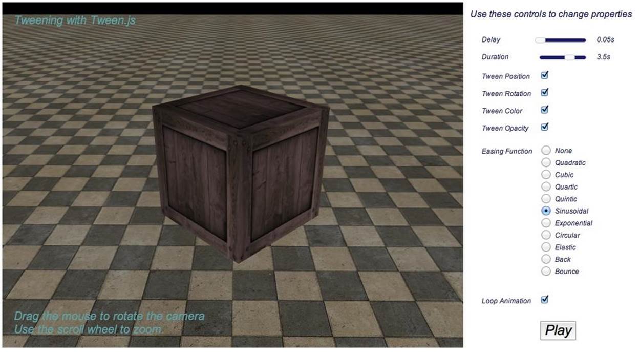
Figure 5-3. Animating transitions with Tween.js

Example 5-3. Tween.js code to animate position

positionTween =

new TWEEN.Tween( group.position )

.to({ x: 2, y: 2, z:-3 }, duration * 1000)

.interpolation(interpolationType)

.delay( delayTime * 1000 )

.easing(easingFunction)

.repeat(repeatCount)

.start();

The position tween is set up with a single chained set of methods:

§ The constructor, new TWEEN.Tween. It takes a single argument, the target object whose properties it will tween.

§ to(), which takes a JavaScript object defining the properties to tween, and a duration in milliseconds.

§ interpolation(), an optional method that specifies the type of interpolation. This can be omitted for linear interpolation, as this is the default (TWEEN.Interpolation.Linear).

§ delay(), an optional method for inserting a delay before the tween starts.

§ easing(), an optional method for applying an easing function (covered in the next section).

§ repeat(), an optional method for specifying the number of times the tween repeats (default is zero).

§ start(), which starts the tween.

Note that these methods can also be called separately. Each of the tweens—position, rotation, material color, and opacity—is set up in a similar fashion. A great thing about Tween.js is that you do not have to supply all values of the object to the to() method, only those that will be changed. For example, the rotation tween changes only the rotation about the y-axis, so it is created as follows:

rotationTween =

new TWEEN.Tween( group.rotation )

.to( { y: Math.PI * 2 }, duration * 1000)

.interpolation(interpolationType)

.delay( delayTime * 1000 )

.easing(easingFunction)

.repeat(repeatCount)

.start();

Once the tween is set up and started, it is now a matter of making sure that Tween.js updates it every animation frame. It is up to the application to do this, so we add the following line to our run() function:

TWEEN.update();

Under the hood, Tween.js keeps a list of all its running tween objects and calls their update() methods in turn. update() calculates how much time has elapsed, applies easing functions and delay and repeat options, and ultimately sets the properties of the target object as specified in theto() method. This is a beautifully elegant yet simple scheme for making object properties change over time without having to handcode the changes each frame.

Easing

Basic tweens with linear interpolation can result in a stiff, unnatural effect, because the objects change at a constant rate. This is unlike objects in the real world, which behave with inertia, momentum, acceleration, and so on. With Tween.js, we can create more natural-feeling tweens by incorporating easing—nonlinear functions applied to the start and end of the tween. Easing is a great tool for adding more realism to your tweens. It can even do a fair job approximating physics without requiring the hard work of integrating a physics engine into your application.

Try out the various easing functions in the tweening sandbox and note their effects. Some simply create a gradual speedup and slowdown of the tween; others provide bouncy and springy effects. The polynomial easing functions Quadratic, Cubic, Quartic, and Quintic ease the tween just as their names imply: via second-, third-, fourth-, and fifth-degree functions. Other easing functions provide sine wave, bounce, and spring effects. Each easing function can be used to ease in (at the beginning of the tween), ease out (at the end of the tween), or do both.

What the easing functions are actually doing is modifying time. Example 5-4 shows the code for the easing function TWEEN.Easing.Cubic. Inputs to the easing functions are in the range [0..1] (i.e., a fraction of the tween’s full duration). The input, k, is cubed by the easing function; therefore, small input values of k return even smaller output values; however, as k approaches 1, so does the return value.

Example 5-4. The Tween.js cubic easing function

Cubic: {

In: function ( k ) {

return k * k * k;

},

Out: function ( k ) {

return --k * k * k + 1;

},

InOut: function ( k ) {

if ( ( k *= 2 ) < 1 ) return 0.5 * k * k * k;

return 0.5 * ( ( k -= 2 ) * k * k + 2 );

}

},

NOTE

The Tween.js easing functions are based on the seminal animation work of Robert Penner. They offer a wide range of powerful easing equations, including linear, quadratic, quartic, sinusoidal, and exponential. Penner’s work has been ported from the original ActionScript to several languages, including JavaScript, Java, CSS, C++, and C#, and has been incorporated into jQuery’s animation utilities.

As we have just seen, tweens are great for easily creating simple, natural-looking effects. Tween.js even lets you chain animations together into a sequence so that you can compose simple effects into more powerful ones. However, as you begin building complex animation sequences you are going to want a more general solution. That’s where key frames come in.

Using Key Frames for Complex Animations

Tweens are perfect for simple transition effects. More complex animations take the tween concept to the next level by using key frames. Rather than specifying a single pair of values to tween, a key frame animation consists of a list of values, with potentially different durations in between each successive value. Note that the term key frame animation is used in both frame-based and time-based systems—a holdover from frame-based nomenclature.

Key frame data consists of two components: a list of time values (keys) and a list of values. The listed values represent the property values to be applied at the time of the corresponding key; the animation system computes tweens for time values lying between any pair of keys.

The following code fragment (from a hypothetical animation engine) shows sample key frame values for an animation that moves an object from the origin up and away from the camera. Over the course of a second, the object moves upward in the first quarter of a second, then up some more and away from the camera in the remaining three-quarters of a second. The animation system will calculate tweens for the points (0, 0, 0) to (0, 1, 0) over the first quarter-second, then tweens for (0, 1, 0) to (0, 2, 5) over the remaining three-quarters of a second.

var keys = [0, 0.25, 1];

var values = [[0, 0, 0],

[0, 1, 0),

[0, 2, 5]

];

Key frame animations can work with linear interpolation, or more complex interpolation such as spline-based; in other words, the data points representing the keys can be thought of as points in a line graph or as the graph of a more complicated function such as a cubic spline. While both tweening and key framing employ interpolation, there are two main aspects that differentiate key frame animations from simple tweens: 1) key frame animations can contain more than two values, and 2) the time interval can vary between successive keys. This enables more powerful effects and gives the animator more control.

Keyframe.js—A Simple Key Frame Animation Utility

Before we can look at a key-framing example, we need to identify an animation library that supports the technique. Tween.js has taken baby steps toward supporting key framing, by allowing lists of property values instead of just pairs. However, in my opinion the syntax for these is a bit cumbersome. Also, there is no way to vary the interval between successive keys. Three.js actually provides built-in animation classes for animating with key frames, but these are not easy to use for handcoding quick and dirty effects; they were built primarily to support the file loading utilities for loading JSON, COLLADA, and other formats. Fair enough: in general, key frame content is meant to be generated by authoring tools such as 3ds Max, Maya, or Blender, not written by hand. Still, it would nice to have an easy way for programmers to put together simple key frames. My frustration with the lack of an easy key framing solution for WebGL led me to write my own utility, Keyframe.js.

Keyframe.js is very simple. It implements two classes, a KeyFrameAnimator class that controls the animation state (start, stop, looping logic, and so on), and an Interpolator class that calculates the tweens for each key pair. At the moment, the library supports only linear interpolation. However, Keyframe.js does allow the programmer to supply easing functions, and for those we can borrow the excellent Penner equations implemented in Tween.js—no need to reinvent the wheel. To see Keyframe.js in action, open the file Chapter 5/keyframeanimation.html. You will see a page that looks like the screenshot in Figure 5-4. Here we see a high seas adventure in progress: a wooden crate bobs in turbulent water, while the sky occasionally brightens and darkens, signaling an impending storm. The controls on the right allow you to play with the duration, turn individual animations on and off, and toggle looping.

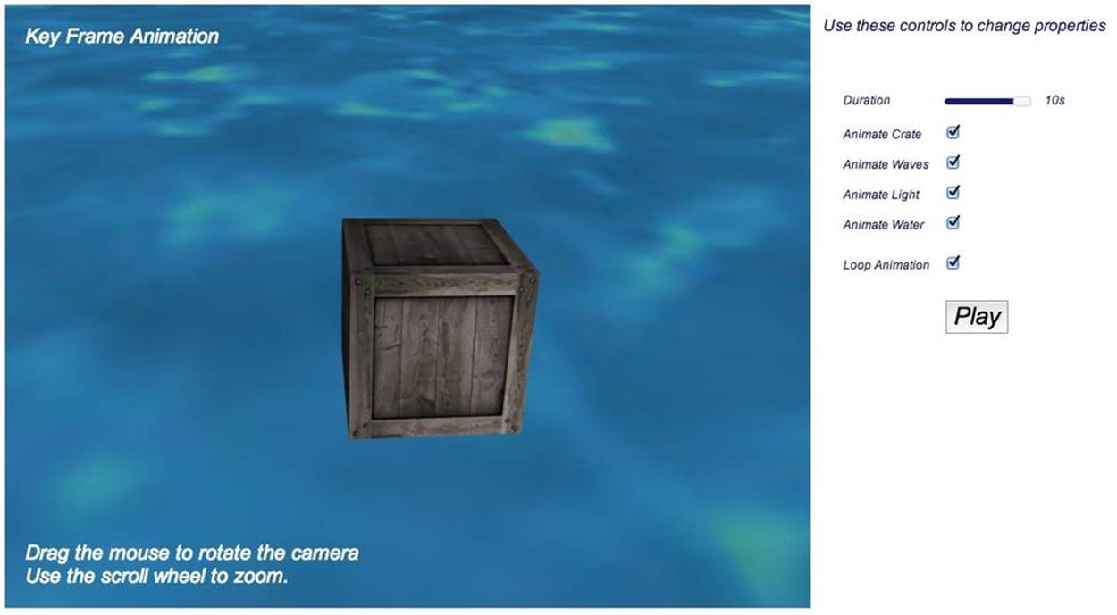
Figure 5-4. Complex animations using key frames

Example 5-5 shows the code to animate the wooden crate. First, we create a new KF.KeyFrameAnimator and initialize it with parameters: looping, a time duration (in milliseconds), an easing function (borrowed from Tween.js), and a set of key frame interpolation data in the parameterinterps. Most notably in contrast with Tween.js, the keys and values are lists, not just pairs; moreover, the intervals between successive keys are different. Following the details of the position interpolator (target:group.position), the crate moves left and forward from time t = 0 to t= 0.2, then back to the origin quickly (t = 0.2 to 0.25), after which it quickly dips into the water (t = 0.25 to 0.375). It then moves back up to the surface at t = 0.5, slowly sinks (t = 0.5 to 0.9), and finally bobs back up at t = 1.0. Note that in Keyframe.js, keys are specified as a fraction of the duration; that is, they always range from 0 to 1, so the actual time of a frame is equal to:

There is a second interpolator for rotation, to tilt the crate about the x-axis. Note that this interpolator has a different number of keys; that is valid, and in fact a feature. The position and rotation animations were created intentionally to be a little out of sync, to make the effect more chaotic. The final flourish is the incorporation of the easing function TWEEN.Easing.Bounce.InOut. The combination of independent, uncoordinated translation and rotation with the bouncy math of the easing function does the trick: the crate does a fair job of appearing to bounce around in the water. The only thing left to do is play the animation, by calling its start() method.

Example 5-5. Key frame animation for the crate

if (animateCrate)

{

crateAnimator = new KF.KeyFrameAnimator;

crateAnimator.init({

interps:

[

{

keys:[0, .2, .25, .375, .5, .9, 1],

values:[

{ x : 0, y:0, z: 0 },

{ x : .5, y:0, z: .5 },

{ x : 0, y:0, z: 0 },

{ x : .5, y:-.25, z: .5 },

{ x : 0, y:0, z: 0 },

{ x : .5, y:-.25, z: .5 },

{ x : 0, y:0, z: 0 },

],

target:group.position

},

{

keys:[0, .25, .5, .75, 1],

values:[

{ x : 0, z : 0 },

{ x : Math.PI / 12, z : Math.PI / 12 },

{ x : 0, z : Math.PI / 12 },

{ x : -Math.PI / 12, z : -Math.PI / 12 },

{ x : 0, z : 0 },

],

target:group.rotation

},

],

loop: loopAnimation,

duration:duration * 1000,

easing:TWEEN.Easing.Bounce.InOut,

});

crateAnimator.start();

}

The animations for the water and storm are handled similarly, though none of the other animations use an easing function. There is an animation to make the water surface move up and down (simple rotation of the water plane about the x-axis); one for creating the appearance of waves, essentially “scrolling” the texture map by interpolating its offset property; and one to make the light flash by interpolating its RGB color values.

This example is a simple illustration of how key frames can create more interesting effects than the basic transitions supported in Tween.js. Key frames can be expressed easily as arrays of keys and values, allowing the animator to sequence tweens of different durations. In practice, programmers rarely create these kinds of animations by hand; rather, artists do it using professional tools. This is the preferred way to go for developing complex effects, especially those involving multiple objects—the subject of the next section.

Articulated Animation with Key Frames

The animation strategies we have discussed so far can be used to move single objects in place (i.e., with rotation) or around and within the scene, but they can also be used to create complex motions in composite objects using a transform hierarchy.

Let’s say we want to create a robot that walks and waves its arms. We would model the robot as a hierarchical structure: the robot body contains an upper body and lower body, the upper body contains arms and a torso, the arms contain upper arms and lower arms, and so on. By properly constructing the hierarchy and animating the right parts, we can get the robot to move its arms and legs. The technique of constructing bodies by combining a hierarchy of discrete parts and animating them in combinations is known as articulated animation.

The Three.js examples come with a nice demonstration of articulated animation. Load the Three.js example file examples/webgl_loader_collada_keyframe.html. You will see an animated model of a pump that shows its inner workings. As the pump rotates, it opens up to assemble and disassemble itself, exposing various parts such as valves, gaskets, gears, housings, and the bolts that hold the pump together. Each of the parts animates individually; however, thanks to the Three.js transform hierarchy, each part also moves with its ancestors as they go through their paces, opening and closing, inserting one part into another, and so on. Figure 5-5 depicts the pump in action.

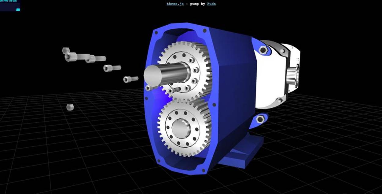
Figure 5-5. Articulated animation: the inner workings of a pump using key frames with a transform hierarchy (COLLADA model created with the Kuda open source authoring system)

This pump model is loaded via the COLLADA file format (.dae file extension), an XML-based text format for describing 3D content. COLLADA can represent individual models or entire scenes, and supports materials, lights, cameras, and animations. We won’t get too deep into the details, but key frame data in COLLADA looks similar to the following excerpt from the pump model (file examples/models/collada/pump/pump.dae):

<animation id="camTrick_G.translate_camTrick_G">

<source id="camTrick_G..." name="camTrick_G...">

<float_array id="camTrick_G..." count="3">0.04166662 ... </float_array>

<source id="camTrick_G..." name="camTrick_G...">

<float_array id="camTrick_G..." count="3">8.637086 ... </float_array>

The COLLADA <animation> element defines an animation. The two <float_array> child elements shown here define the keys and values, respectively, required to animate the x component of the transform for an object named camTrick_G. The keys are specified in seconds. Over the course of 7.08333 seconds, camTrick_G will translate in x from 8.637086 to 0. There is an additional key in between at 6.5 seconds that specifies an x translation of 7.794443. So, for this animation, there is a rather slow x translation over the first 6.5 seconds, followed by a rapid one over the remaining 0.58333 seconds. There are dozens of such animation elements defined in this COLLADA file (74 in all) for the various objects that compose the pump model.

Example 5-6 shows an excerpt from the code that sets up the animations for this example. The example makes use of the built-in Three.js classes THREE.KeyFrameAnimation and THREE.AnimationHandler. THREE.KeyFrameAnimation implements general-purpose key frame animation for use with COLLADA and other animation-capable formats. THREE.AnimationHandler is a singleton that manages a list of the animations in the scene and maintains responsibility for updating them each time through the application’s run loop. (The code for these classes can be found in the Three.js project in the folder src/extras/animation.)

Example 5-6. Initializing Three.js key frame animations

var animHandler = THREE.AnimationHandler;

for ( var i = 0; i < kfAnimationsLength; ++i ) {

var animation = animations[ i ];

animHandler.add( animation );

var kfAnimation = new THREE.KeyFrameAnimation(

animation.node, animation.name );

kfAnimation.timeScale = 1;

kfAnimations.push( kfAnimation );

}

The example does a little more setup before eventually calling each animation’s play() method to get it running. play() takes two arguments: a loop flag and an optional start time (with zero, the default, meaning play immediately):

animation.play( false, 0 );

This example shows how key frame animation can combine with a transform hierarchy to create complex, articulated effects. Articulated animation is typically used as the basis for animating mechanical objects; however, as we will see later in this chapter, it is also essential for driving the skeletons underlying skinned animation.

NOTE

As is the case with many of the file format loaders that come with Three.js, the COLLADA loader is not part of the core package but rather included with the samples. The source code for the Three.js COLLADA loader can be found in examples/js/loaders/ColladaLoader.js. The COLLADA format will be discussed in detail in Chapter 8.

Using Curves and Path Following to Create Smooth, Natural Motion

Key frames are the perfect way to specify a sequence of transitions with varying time intervals. By combining articulated animation with hierarchy, we can create complex interactions. However, the samples we have looked at so far look mechanical and artificial because they use linear functions to interpolate. The real world has curves: cars hug curved roads, planes travel in curved paths, projectiles fall in an arc, and so on. Attempting to simulate those effects using linear interpolation produces unsettling, unnatural results. We could use a physics engine, but for many uses that is overkill. Sometimes we just want to create a predefined animation that looks natural, without having to pay the costs of computing a physics simulation.

Key frame data is not just limited to describing linear animations. It can be treated as points on a curve, too. The most common type of curve used in animation is a spline curve—a smooth, continuous curve. Certain types of splines, called B-splines, are common in computer graphics because they are relatively fast to compute. We define a B-spline using a set of data points to define the basic shape of the curve, plus additional control points that modulate the shape of the curve. The simple B-spline depicted in Figure 5-6 shows the control points in black. If you have ever used a professional drawing program such as Adobe Illustrator, you will be familiar with control points used to modify the shape of a spline curve.

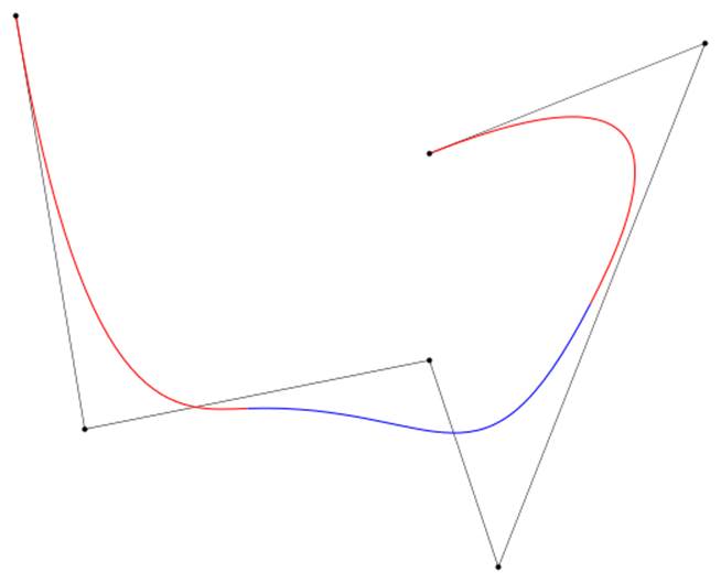
Figure 5-6. A B-spline curve, by Wojciech mula (licensed under Creative Commons CC0 1.0 Universal Public Domain Dedication)

Spline interpolation is more complex than simple linear interpolation, incorporating polynomial formulas akin to those found in the Tween.js easing functions, and an additional value on either side of the key values to compute the smooth curve. A full explanation of spline interpolation mathematics is beyond the scope of this book. However, Figure 5-7 shows an intuitive view of how it works: to compute an interpolated value along the curve between points P1 and P2, we also use control points P0 and P3 in order to generate a value that lies on the spline curve.

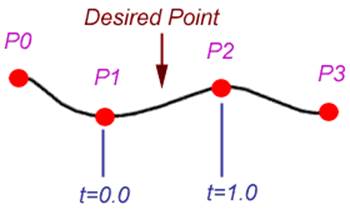
Figure 5-7. Spline interpolation; reproduced with permission

NOTE

Splines come in several varieties, including B-splines, cubic Bézier splines, and Catmull-Rom splines, named after animation genius and Pixar founder Ed Catmull. Catmull-Rom has become popular because it is easier to construct and compute than Bézier curves. Three.js comes with a built-in animation class that uses Catmull-Rom interpolation. See the Three.js source filesrc/extras/animations/animation.js.

There are several good online Catmull-Rom tutorials, including http://flashcove.net/795/cubic-spline-generation-in-as3-catmull-rom-curves/ and http://www.mvps.org/directx/articles/catmull/.

Spline animation often needs to take into account orientation as well as position. If, for example, you want to animate an object following a curved path, you need to have it turn, tilt, and roll in order to make it appear natural. That involves computing a new orientation at each point. Figure 5-8 depicts that process. At each point on the curve, a tangent, normal, and binormal are computed. Informally, the tangent is the straight line following the direction of the curve, intersecting it at one point only. The normal is the line perpendicular to the direction of the curve (and to the tangent). The binormal is the cross product of the other two lines. Together, these three vectors define a frame of reference known as the TNB frame, which defines the orientation for an object following the path.

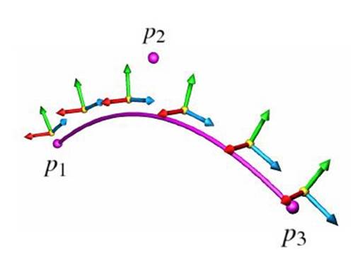
Figure 5-8. Coordinate frames for spline animation; tangents, normals, and binormals are represented by blue (forward), green (up), and red (right) arrows, respectively; image courtesy Cedric Bazillou, reproduced with permission

There is a nice example of path-following animation in the Three.js samples. Open the file examples/webgl_geometry_extrude_splines.html. Be sure to press the button labeled Camera Spline Animation View to see the animation depicted in Figure 5-9. The camera follows the spline curve from a short distance away, continually adjusting its position and orientation. This particular example was animated programmatically, computing the spline interpolation and TNB frame in code. But it could conceivably be packaged into a reusable path-following animation class.

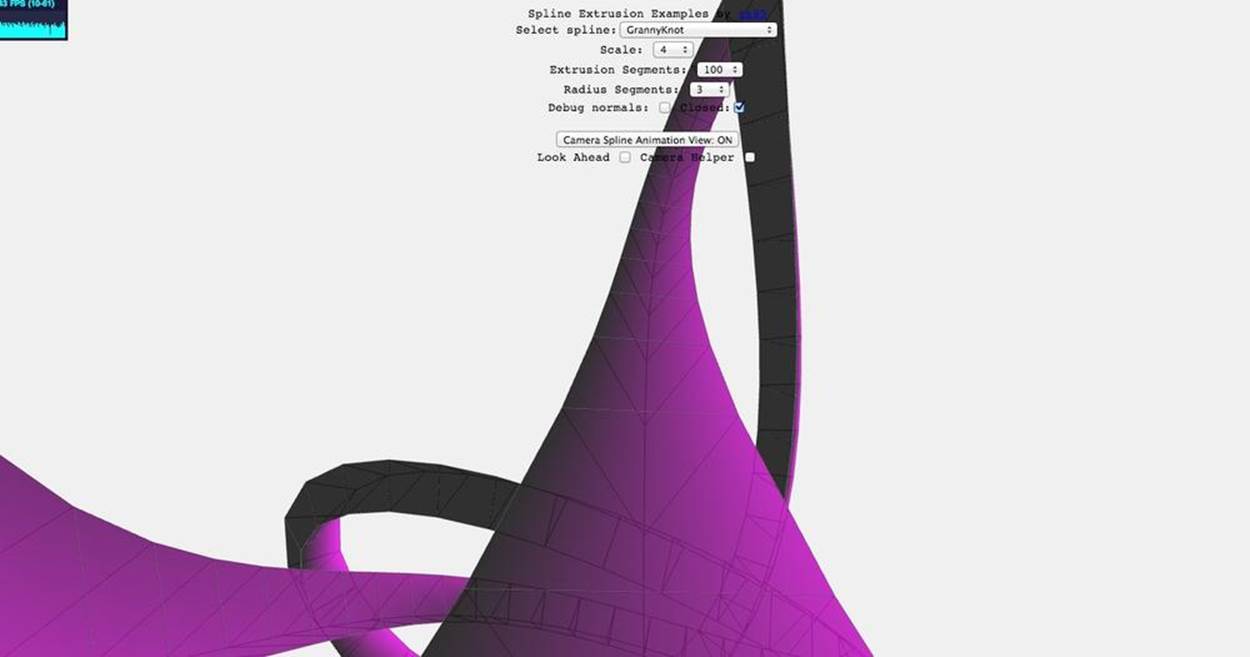
Figure 5-9. A camera animating along a path

Using Morph Targets for Character and Facial Animation

Key frames and articulated animation are great for moving objects around within the scene, but many animation effects require changing the geometry of the object itself. A common way to do this is via morph target animation, or simply, morphing. Morphing uses vertex-based interpolations to change the vertices of a mesh. Typically, a subset of the vertices of a mesh is stored, along with their indices, as a set of morph targets to be used in a tween. The tween interpolates between each of the vertex values in the morph targets, and the animation uses the interpolated values to deform the vertices in the mesh.

Morph targets are excellent for facial expressions and other fine details that are not so easy to implement in a skinned animation (see next section); they are compact and don’t require a highly detailed skeleton with numerous facial bones. In addition, they allow the animator to create very specific expressions by tweaking the mesh right down the vertex level. Figure 5-10 illustrates the use of morphing to create facial expressions. Each different expression, such as the pursed lips or the smile, is represented by a set of vertices including the mouth and surrounding areas.

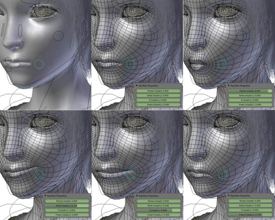
Figure 5-10. Facial morphs; Creative Commons Attribution-Share Alike 3.0 unported license

Morphs can be used for more than just faces. Several examples in the Three.js project use morph targets to animate entire characters. Figure 5-11 depicts characters animated using morphs. These characters were originally modeled in the id Software MD2 file format, a popular morph-based format used for animating player characters in id games such as Quake II. The MD2 file was then converted to the Three.js JSON file format (see Chapter 8).

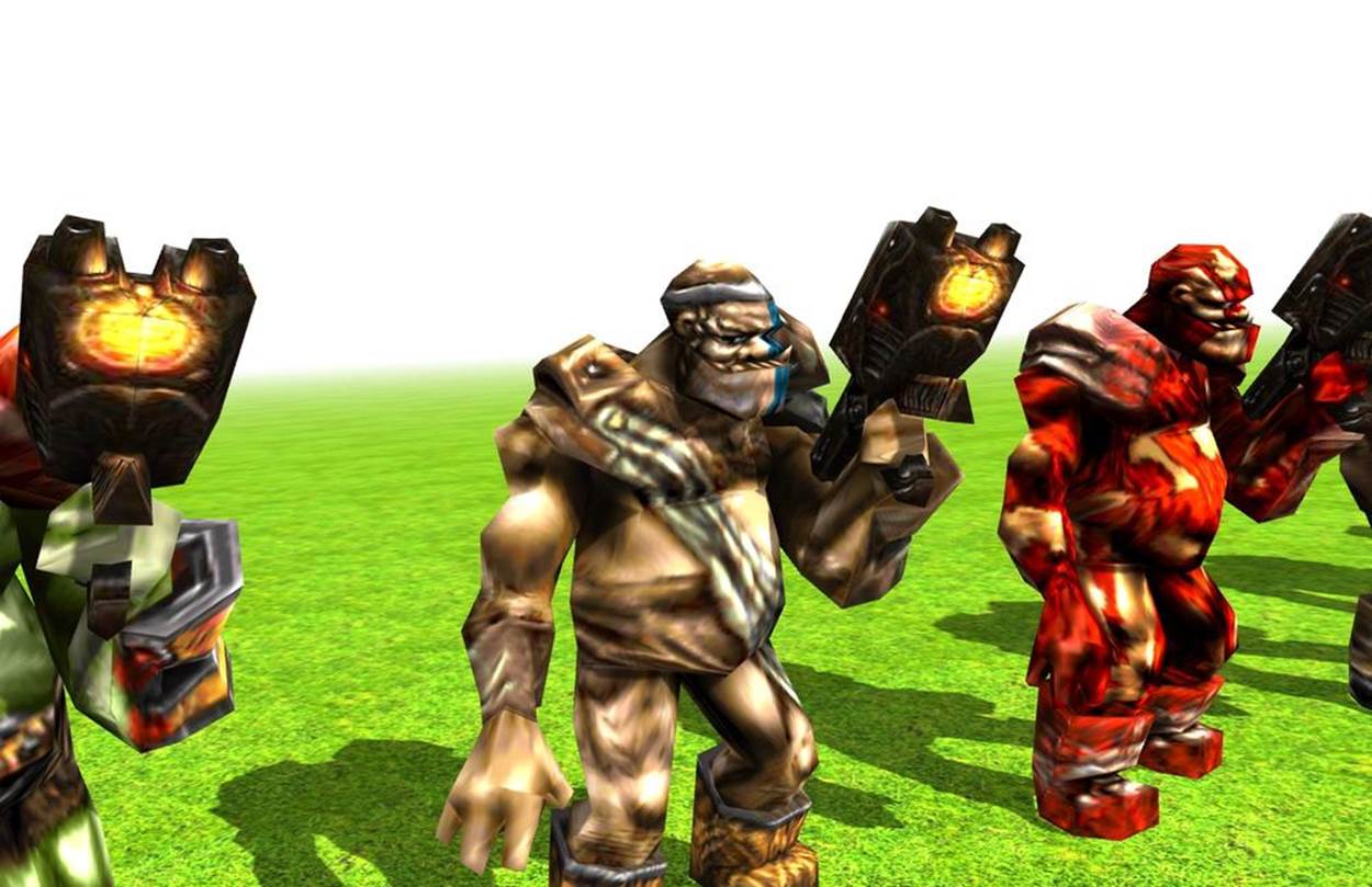
Figure 5-11. Animating characters with morph targets; models converted from MD2 format to Three.js JSON (“Ogro” character by Magarnigal)

To see these animations, load the file examples/webgl_morphtargets_md2_control.htm. You will see several ogre characters lumbering, turning, and looking over their shoulders. The arrow and WASD keys on the keyboard will make the characters move around the scene, transitioning from their idle animations to walking and turning animation sequences. The effect is quite convincing.

To get a feel for what morph target data looks like, open the converted MD2 file located in examples/models/animated/ogro/ogro-light.js. At around line 18, you will see a JSON property that begins as follows:

"morphTargets": [

{ "name": "stand001", "vertices": [0.6,-2.7,1.5,-5.5,-3.3,-0.6 ...

This continues for several lines. Each element of the morphTargets array is a single morph target; each morph target contains the complete set of vertices for the ogre mesh, but with different position values. Three.js animates the morph by cycling through the set of targets for the model, interpolating vertex values to blend from one target to the next. You can find the code for loading, setting up, and animating MD2 characters implemented in the class THREE.MD2CharacterComplex, in the Three.js example source file examples/js/MD2CharacterComplex.js.

NOTE

The MD2 file for this example was converted to the Three.js JSON file format using a wonderful online utility written by Klas, aka OutsideOfSociety, a team member at Swedish-based interactive developer North Kingdom. For details on how to use the converter, see Klas’s blog entry.

Animating Characters with Skinning

Articulated animation works very well for inorganic objects—robots, cars, machines, and so on. It breaks down badly for organic objects. Plants swaying in the breeze, animals bounding, and people dancing all involve changes to the geometry of a mesh: branches twist, skin ripples, muscles bulge. It is nearly impossible to do this well with the tinker-toy approach that is articulated animation. So we turn to another technique called skinned animation, also known as skinning, skeletal animation, or single mesh animation.

Skinned animation involves deforming the actual vertices of a mesh, or skin, over time. Animation is driven by an articulated object hierarchy known as a skeleton (sometimes called a rig). The skeleton is used only as the underlying mechanism for animating; we don’t see it on the screen. Changes to the skeleton, combined with additional data describing how the skeleton influences changes to the skin in various regions of the mesh, drive the skinned animation. Figure 5-12 depicts a simple skeleton and its associated skin.

A skeleton is composed, not surprisingly, of bones. Bones are organized in a hierarchy, in the intuitive way you would expect. Like the old song goes: foot bone connected to the leg bone, leg bone connected to the knee bone…and so on. Just as with articulated animation, transforming a bone moves all its child bones. However, unlike with articulated animation, the skeleton is not visible.

Each bone in the skeleton is associated with a set of vertices of the mesh, along with a blend weight (also known as a vertex weight) for each associated vertex. The blend weight specifies how much that particular bone influences its associated vertices. Vertices can be associated with multiple bones, so the ultimate position and orientation of a vertex is determined by the combined transformations of all associated bones, scaled by the respective weights. If this sounds complicated, it is. Skinned animations are almost always produced by authoring tools rather than created by hand. They are also algorithmically complex; these days, most runtime engines animate skins using the GPU if possible. This includes Three.js.

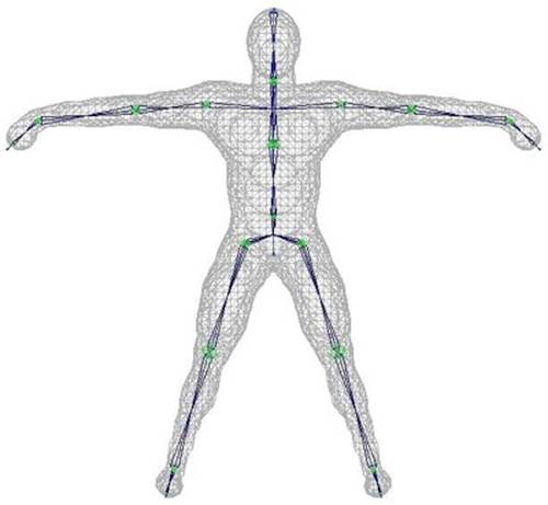
Figure 5-12. A character mesh with underlying skeleton, suitable for skinned animation—from a tutorial on skinning by Frank A. Rivera

To see an example of skinned animation in action, open the file under the Three.js project located in examples/webgl_animation_skinning.html. You will see many instances of a buffalo model. Click to start the animation; the buffalo will run in place with natural-looking movement. SeeFigure 5-13.

Let’s walk through a portion of the code for this sample to see how Three.js implements skinning. First, we load the buffalo model by creating a new THREE.JSONLoader object and calling its load() method. This class loads files in the Three.js JSON file format. The format contains skinning information as well as the geometry.

var loader = new THREE.JSONLoader();

loader.load( "obj/buffalo/buffalo.js", createScene );

load() takes as its second argument a callback function that will be invoked once the file has been downloaded and parsed. Example 5-7 shows an excerpt from the callback function createScene(), with the relevant lines highlighted in bold.

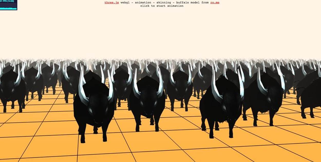
Figure 5-13. Meshes animated using skinning in Three.js; buffalo model from RO.ME

Example 5-7. Callback to set up skinned animation after file load

function createScene( geometry, materials ) {

buffalos = [];

animations = [];

var x, y,

buffalo, animation,

gridx = 25, gridz = 15,

sepx = 150, sepz = 300;

var material = new THREE.MeshFaceMaterial( materials );

var originalMaterial = materials[ 0 ];

originalMaterial.skinning = true;

originalMaterial.transparent = true;

originalMaterial.alphaTest = 0.75;

THREE.AnimationHandler.add( geometry.animation );

for( x = 0; x < gridx; x ++ ) {

for( z = 0; z < gridz; z ++ ) {

buffalo = new THREE.SkinnedMesh( geometry,

material, false );

buffalo.position.x = - ( gridx - 1 ) * sepx * 0.5 +

x * sepx + Math.random() * 0.5 * sepx;

buffalo.position.z = - ( gridz - 1 ) * sepz * 0.5 +

z * sepz + Math.random() * 0.5 * sepz - 500;

buffalo.position.y =

buffalo.geometry.boundingSphere.radius * 0.5;

buffalo.rotation.y = 0.2 - Math.random() * 0.4;

scene.add( buffalo );

buffalos.push( buffalo );

animation = new THREE.Animation( buffalo, "take_001" );

animations.push( animation );

offset.push( Math.random() );

}

createScene() runs a loop to create many instances of a buffalo mesh from the one loaded geometry. Note the type of mesh created: instead of the THREE.Mesh type we are familiar with from previous examples, this uses a different kind of mesh: THREE.SkinnedMesh. This particular Three.js type will be rendered via a special vertex shader that performs skinned animation on the GPU for performance.

createScene() also uses the built-in Three.js animation classes THREE.Animation and THREE.AnimationHandler. THREE.Animation is a class that implements general-purpose key frame animation, which in the case of skinning, is used to drive the skeleton animation.THREE.AnimationHandler is a singleton object that stores all animations for a scene, and maintains responsibility for updating them each time through the application’s run loop. Our callback first adds the animation data to the animation handler’s list by callingTHREE.AnimationHandler.add(), passing it the geometry’s animation data, which was loaded automatically by the Three.js JSON loader. A little later, the code creates a new THREE.Animation for each buffalo instance, associating the instance stored in variable buffalo with the animation named "take_001" from the JSON file.

After the animations are set up, we are ready to play them. The application does this by calling the function startAnimation() when the mouse is clicked. See Example 5-8. startAnimation() loops through the array of animations, calling play() on each. Each animation is also given a different, random time offset, to keep the animals from being perfectly synchronized.

Example 5-8. Playing the skinned animations

function startAnimation() {

for( var i = 0; i < animations.length; i ++ ) {

animations[ i ].offset = 0.05 * Math.random();

animations[ i ].play();

}

dz = dstep;

playback = true;

}

If you are interested in the details of the JSON animation format, look at the file examples/obj/buffalo.js. Search through the file for the properties bones, skinWeights, and skinIndices to see how the skeleton data is laid out; also look for the property animation, which contains the hierarchy of key frames used to animate the skeleton. There is a lot going on under the covers, and Three.js adds a lot of value, not the least of which is a shader-based implementation of skinning that relies on the GPU for computation.

Animating Using Shaders

The techniques we have explored thus far in this chapter, such as key frames, tweens, and skinning, can be implemented in JavaScript, but you can also develop them using GLSL programmable shaders to obtain hardware-accelerated performance. The animation support in the Three.js library uses both strategies: the key frame system is pure JavaScript, while the morphing and skinning are implemented as part of the built-in shader code for Three.js built-in material types such as Phong and Lambert. If skinning or morphing data is present in the mesh (usingTHREE.SkinnedMesh, described earlier, or THREE.MorphAnimMesh), then the Three.js shader will use that information to calculate new vertex positions.

NOTE

If you are interested in the details of Three.js’s GLSL skinning and morphing code, open the Three.js source file src/renderers/WebGLShaders.js and search for “skin” and “morph”—but be advised that this gets deep into both the GLSL language and the specifics of the Three.js implementation. If you do manage to get around in there, it will be worth it, as there is a wealth of information.

Beyond using the GPU to optimize performance of common techniques like skinning, we can also write GLSL code to create arbitrary effects. Perhaps we want make the surface of an ocean shimmer, to simulate light reflecting and refracting as the waves undulate; or maybe we want to create grass that sways in the breeze. We could code these effects purely in JavaScript, but GLSL is much better suited to manipulating the large amounts of vertex and image data involved. The Three.js project comes with an excellent example of shader-based animation. Open the example fileexamples/webgl_shader_lava.html. You will see a torus shape, slowly rotating, with a flowing lava surface. See Figure 5-14.

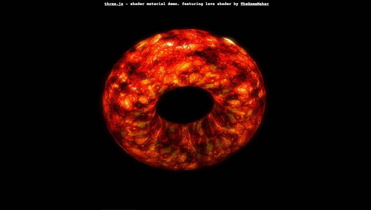
Figure 5-14. Animated lava effect using a GLSL shader; shader code by TheGameMaker

The lava flow is animated via a THREE.ShaderMaterial with custom GLSL code. Let’s have a look. Example 5-9 shows the code to set up the ShaderMaterial. There are several uniform values passed to the shader. The important ones for our purposes are time and the two texture maps, texture1 and texture2. As we will see momentarily, those three parameters, plus a little magic with numbers, are all we need to create realistic-looking, flowing lava.

Example 5-9. Creating the torus mesh and ShaderMaterial

uniforms = {

fogDensity: { type: "f", value: 0.45 },

fogColor: { type: "v3",

value: new THREE.Vector3( 0, 0, 0 ) },

time: { type: "f", value: 1.0 },

resolution: { type: "v2",

value: new THREE.Vector2() },

uvScale: { type: "v2",

value: new THREE.Vector2( 3.0, 1.0 ) },

texture1: { type: "t",

value: THREE.ImageUtils.loadTexture(

"textures/lava/cloud.png" ) },

texture2: { type: "t",

value: THREE.ImageUtils.loadTexture(

"textures/lava/lavatile.jpg" ) }

};

uniforms.texture1.value.wrapS =

uniforms.texture1.value.wrapT = THREE.RepeatWrapping;

uniforms.texture2.value.wrapS =

uniforms.texture2.value.wrapT = THREE.RepeatWrapping;

Now that the uniforms are set up, we can create the shader material. We need to supply vertex and fragment shader GLSL code to the constructor. Note the following technique for doing this: we use <script> elements in the HTML to hold the GLSL source code, and retrieve thetextContent property of the script to get the GLSL text. Contrast this with previous shader examples we have seen. Rather than having to construct multiline text strings with escaped newlines, we can write the shader code in a straightforward manner. We will look at the GLSL source code in a moment.

var size = 0.65;

material = new THREE.ShaderMaterial( {

uniforms: uniforms,

vertexShader: document.getElementById(

'vertexShader' ).textContent,

fragmentShader: document.getElementById(

'fragmentShader' ).textContent

} );

We then create the torus mesh with the new THREE.ShaderMaterial and add it to the scene:

mesh = new THREE.Mesh(

new THREE.TorusGeometry( size, 0.3, 30, 30 ),

material );

mesh.rotation.x = 0.3;

scene.add( mesh );

The shader algorithm is quite clever. It combines two texture maps, one for the base lava color and visual pattern, and a cloud texture as a source of “noise” that perturbs the base texture over time to create the flowing effect. The two textures are depicted in Figure 5-15.

The GLSL code for the vertex shader is simple; see Example 5-10. As with most shaders, it does the transformation math to multiply vertices by the model, view, and projection matrices to get them into screen space and outputs this value in the built-in GLSL variable gl_Position. Beyond that, we declare a varying parameter, vUv. This is the texture coordinate at each vertex, which the vertex shader outputs for use in the fragment shader, as we will see shortly. This particular shader also allows a scale parameter to be passed in, which it uses to scale the texture coordinates.

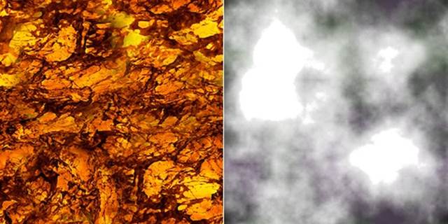
Figure 5-15. Texture maps for lava and noise

As noted, the GLSL source is embedded in a <script> element, so we can easily read the code without all the clutter of quotation marks, newline characters, and the like. The trick here is to use a different script type property, in this case x-shader/x-vertex. The browser has no idea what this type is; we just use it to indicate that this is not a JavaScript language script.

Example 5-10. Vertex shader code embedded in an HTML <script> element

<script id="vertexShader" type="x-shader/x-vertex">

uniform vec2 uvScale;

varying vec2 vUv;

void main()

{

vUv = uvScale * uv;

vec4 mvPosition = modelViewMatrix * vec4( position, 1.0 );

gl_Position = projectionMatrix * mvPosition;

}

</script>

The GLSL code for the fragment shader does most of the work. Example 5-11 shows the code. After declaring uniform parameters to match those in the JavaScript, we declare a varying parameter, vUv, to match the output of the vertex shader.

Example 5-11. Fragment shader code for the shader-based animation

<script id="fragmentShader" type="x-shader/x-fragment">

uniform float time;

uniform vec2 resolution;

uniform float fogDensity;

uniform vec3 fogColor;

uniform sampler2D texture1;

uniform sampler2D texture2;

varying vec2 vUv;

Now for the main fragment shader program. The gist of it is that texture1, the cloud texture, is used as a source of noise to slightly displace the texture coordinate value used to get color values from texture2, the lava texture. (The GLSL function texture2D() fetches color data from a texture, given a 2D texture coordinate.) By multiplying the noise texture coordinate by the current time value, and adding some empirically determined offsets (e.g., 1.5, −1.5), we get the flowing effect. The color value for the pixel is then saved to the built-in GLSL variable gl_FragColor.

void main( void ) {

vec2 position = −1.0 + 2.0 * vUv;

vec4 noise = texture2D( texture1, vUv );

vec2 T1 = vUv + vec2( 1.5, −1.5 ) * time *0.02;

vec2 T2 = vUv + vec2( −0.5, 2.0 ) * time * 0.01;

T1.x += noise.x * 2.0;

T1.y += noise.y * 2.0;

T2.x −= noise.y * 0.2;

T2.y += noise.z * 0.2;

float p = texture2D( texture1, T1 * 2.0 ).a;

vec4 color = texture2D( texture2, T2 * 2.0 );

vec4 temp = color * ( vec4( p, p, p, p ) * 2.0 ) +

( color * color - 0.1 );

if( temp.r > 1.0 ){ temp.bg += clamp( temp.r - 2.0, 0.0, 100.0 ); }

if( temp.g > 1.0 ){ temp.rb += temp.g - 1.0; }

if( temp.b > 1.0 ){ temp.rg += temp.b - 1.0; }

gl_FragColor = temp;

At this point, the flowing lava effect is complete. However, this shader also adds a fog effect. The value stored in gl_FragColor is then mixed with a fog value calculated from fog parameters passed to the shader. The final color value for the pixel is output in the built-in GLSL variablegl_FragColor, and we are finished.

float depth = gl_FragCoord.z / gl_FragCoord.w;

const float LOG2 = 1.442695;

float fogFactor = exp2( - fogDensity * fogDensity * depth *

depth * LOG2 );

fogFactor = 1.0 - clamp( fogFactor, 0.0, 1.0 );

gl_FragColor = mix( gl_FragColor,

vec4( fogColor, gl_FragColor.w ), fogFactor );

}

</script>

The only piece remaining is to drive the animation during our run loop by updating the value of time each time through. Three.js makes this trivial; it automatically passes all uniform values to the GLSL shaders each time the renderer updates. All we need to do is set a property in the JavaScript. In this example, the function render() is called each animation frame. See the line of code in bold.

function render() {

var delta = 5 * clock.getDelta();

uniforms.time.value += 0.2 * delta;

mesh.rotation.y += 0.0125 * delta;

mesh.rotation.x += 0.05 * delta;

renderer.clear();

composer.render( 0.01 );

}

Admittedly, coding an animation like this requires a certain level of artistry. Not only must we learn the details of GLSL syntax and built-in functions, but we must also master some esoteric computer graphics algorithms. But if you have the appetite, it can be really rewarding. And the Internet is full of information and readily usable code examples to get started.

Chapter Summary

As we have seen, there are many ways to animate 3D content in WebGL. At its core, animation is driven by the new browser function requestAnimationFrame(), the workhorse that ensures user drawing happens in a timely and consistent manner throughout the page. Beyond that, we have several choices for animating, ranging from simple to complex, depending on the desired effect. Content can be animated programmatically each frame, or we can use data-driven methods that include tweening, key framing, morphs, and skinning. We can achieve naturalistic motion by combining key frames with path following. We can also use shaders to animate content in the GPU, enabling even more possibilities. The tools and libraries for animating WebGL are still evolving, with no one clear choice. But there are many possibilities and, thanks to JavaScript and open source, few barriers to getting going.