Mastering Structured Data on the Semantic Web From HTML5 Microdata to Linked Open Data(2015)
CHAPTER 6
Graph Databases
Graph models and algorithms are ubiquitous, due to their suitability for knowledge representation in e-commerce, social media networks, research, computer networks, electronics, as well as for maximum flow problems, route problems, and web searches. Graph databases are databases with Create, Read, Update, and Delete (CRUD) methods exposing a graph data model, such as property graphs (containing nodes and relationships), hypergraphs (a relationship can connect any number of nodes), RDF triples (subject-predicate-object), or quads (named graph-subject-predicate-object). Graph databases are usually designed for online transactional processing (OLTP) systems and optimized for transactional performance, integrity, and availability. Unlike relational and NoSQL databases, purpose-build graph databases, including triplestores and quadstores, do not rely on indices, because graphs naturally provide an adjacency index, and relationships attached to a node provide a direct connection to other related nodes. Graph queries are performed using this locality to traverse through the graph, which can be carried out with several orders of magnitude higher efficiency than that of relational databases joining data through a global index. In fact, most graph databases are so powerful that they are suitable even for Big Data applications.
Graph Databases
To leverage the power of the Resource Description Framework (RDF), data on the Semantic Web can be stored in graph databases rather than relational databases. A graph database is a database that stores RDF statements and implements graph structures for semantic queries, using nodes, edges, and properties to represent and retrieve data. A few graph databases are based on relational databases, while most are purpose-built from the ground up for storing and retrieving RDF statements.
There are two important properties of graph databases that determine efficiency and implementation potential. The first one is the storage, which can be native graph storage or a database engine that transforms an RDF graph to relational, object-oriented, or general-purpose database structures. The other main property is the processing engine. True graph databases implement so-called index-free adjacency, whereby connected nodes are physically linked to each other in the database. Because every element contains a direct pointer to its adjacent element, no index lookups are necessary. Graph databases store arbitrarily complex RDF graphs by simple abstraction of the graph nodes and relationships. Unlike other database management systems, graph databases do not use inferred connections between entities using foreign keys, as in relational databases, or other data, such as the ones used in MapReduce. The computational algorithms are implemented as graph compute engines, which identify clusters and answer queries.
One of the main advantages of graph databases over relational databases and NoSQL stores is performance [1]. Graph databases are typically thousands of times more powerful than conventional databases in terms of indexing, computing power, storage, and querying. In contrast to relational databases, where the query performance on data relations decreases as the dataset grows, the performance of graph databases remains relatively constant.
While relational databases require a comprehensive data model about the knowledge domain up front, graph databases are inherently flexible, because graphs can be extended with new nodes and new relationship types effortlessly, while subgraphs merge naturally to their supergraph.
Because graph databases implement freely available standards such as RDF for data modeling and SPARQL for querying, the storage is usually free of proprietary formats and third-party dependencies. Another big advantage of graph databases is the option to use arbitrary external vocabularies and schemas, while the data is available programmatically through Application Programming Interfaces (APIs) and powerful queries.
![]() Note Some graph databases have limitations when it comes to storing and retrieving RDF triples or quads, because the underlying model not always covers the features of RDF well, as for example, using URIs as identifiers is not the default scenario, and the naming convention often differs from that of RDF. Most graph databases do not support SPARQL out of the box, although many provide a SPARQL add-on. The proprietary query languages introduced by graph database vendors are not standardized like SPARQL.
Note Some graph databases have limitations when it comes to storing and retrieving RDF triples or quads, because the underlying model not always covers the features of RDF well, as for example, using URIs as identifiers is not the default scenario, and the naming convention often differs from that of RDF. Most graph databases do not support SPARQL out of the box, although many provide a SPARQL add-on. The proprietary query languages introduced by graph database vendors are not standardized like SPARQL.
The widely adopted relational databases were originally designed to store data such as tabular structures in an organized manner. The irony of relational databases is that their performance is rather poor when handling ad hoc relationships. For example, the foreign keys of relational databases mean development and maintenance overhead, while they are vital for the database to work. Joining two tables in a relational database might increase complexity by mixing the foreign key metadata with business data. Even simple queries might be computationally complex. The handling of sparse tables in relational databases is poor. Regarding NoSQL databases, including key-value-, document-, and column-oriented databases, the relationship handling is not perfect either. Because NoSQL databases typically store sets of disconnected documents, values, or columns (depending on the type), they are not ideal for storing data interconnections and graphs.
The main parameters of graph databases are the load rate in triples/second or quads/second (sometimes combined with the indexing time) and the query execution time. Further features that can be used for comparing graph databases are licensing, source availability (open source, binary distribution, or both), scalability, graph model, schema model, API, proprietary query language and query method, supported platforms, consistency, support for distributed processing, partitioning, extensibility, visualizing tools, storage back end (persistency), language, and backup/restore options. The comparison of the most commonly used graph databases is summarized in Table 6-1.
Table 6-1. Comparison of Common Graph Databases [2]
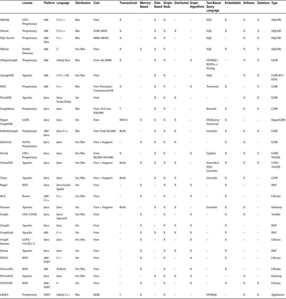
While graph database vendors often compare their products to other graph databases, the de facto industry standard for benchmarking RDF databases is the Lehigh University Benchmark (LUBM), which is suitable for performance comparisons [3].
Triplestores
All graph databases designed for storing RDF triples are called triplestores or subject-predicate-object databases, however, the triplestores that have been built on top of existing commercial relational database engines (such as SQL-based databases) are typically not as efficient as the native triplestores with a database engine built from scratch for storing and retrieving RDF triples. The performance of native triplestores is usually better, due to the difficulty of mapping the graph-based RDF model to SQL or NoSQL queries.
The advantages of graph databases are derived from the advantageous features of RDF, OWL, and SPARQL. RDF data elements are globally unique and linked, leveraging the advantages of the graph structure. Adding a new schema element is as easy as inserting a triple with a new predicate. Graph databases also support ad hoc SPARQL queries. Unlike the column headers, foreign keys, or constraints of relational databases, the entities of graph databases are categorized with classes; predicates are properties or relationships; and they are all part of the data. Due to the RDF implementation, graph databases support automatic inferencing for knowledge discovery. The data stored in these databases can unify vocabularies, dictionaries, and taxonomies through machine-readable ontologies. Graph databases are commonly used in semantic data integration, social network analysis, and Linked Open Data applications.
Quadstores
It is not always possible to interpret RDF statements without a graph identifier. For example, if a given name is used as a subject, it is out of context if we do not state the person we want to describe. If, however, we add the web site address of the same person to each triple that describes the same person, all components become globally unique and dereferenceable. A quad is a subject-predicate-object triple coupled with a graph identifier. The identified graph is called a named graph.
For example, consider an LOD dataset description in a Turtle file registered on datahub.io, such as http://www.lesliesikos.com/datasets/sikos-void.ttl. To make RDF statements about the dataset graph, the subject is set to the file name and extension of the RDF file representing the graph (http://www.lesliesikos.com/datasets/sikos.rdf). This makes it possible to write RDF statements about the file, describing it as an LOD dataset (void:Dataset), adding a human-readable title to it using Dublin Core (dc:title), declaring its creator (dc:creator), and so on, as shown in Figure 6-1.
![]() Caution Notice the difference between http://www.lesliesikos.com/datasets/sikos.rdf and http://www.lesliesikos.com/datasets/sikos.rdf#sikos. The first example refers to a file; the second refers to a person described in the file.
Caution Notice the difference between http://www.lesliesikos.com/datasets/sikos.rdf and http://www.lesliesikos.com/datasets/sikos.rdf#sikos. The first example refers to a file; the second refers to a person described in the file.
If a graph database stores the graph name (representing the graph context or provenance information) for each triple, the database is called a quadstore.
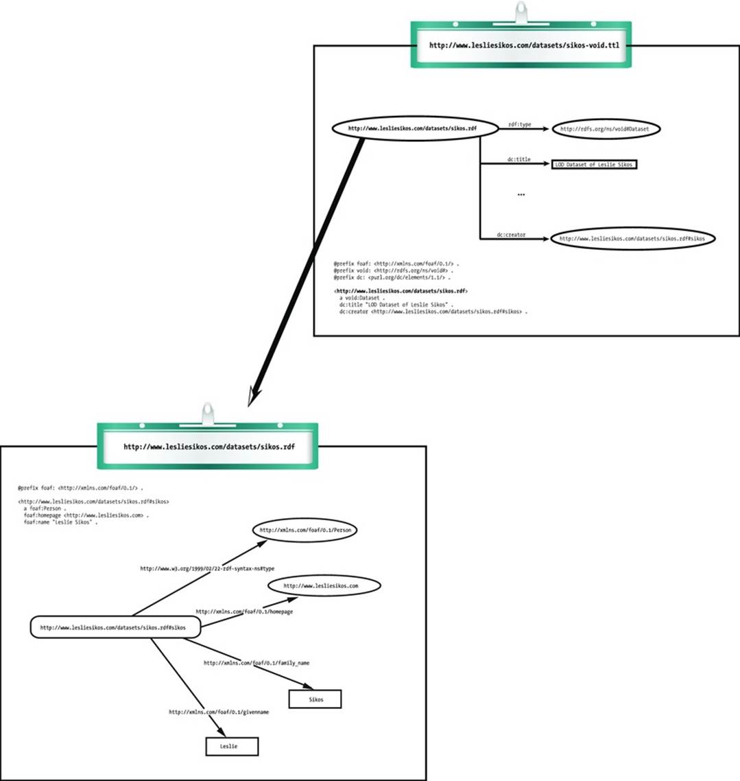
Figure 6-1. Referencing from a named graph to another named graph
The Most Popular Graph Databases
Some of the most widely deployed, high-performance graph databases are AllegroGraph, Neo4j, Blazegraph (formerly Big Data), OpenLink Virtuoso, Clark & Parsia’s Stardog, BigOWLIM, 4Store, YARS2, Jena TDB, RDFox, Jena SDB, Mulgara, RDF Gateway, Kowari, and Sesame. However, not everyone uses a native graph database engine to store triples or quads. Some examples are Oracle Spatial and Graph with Oracle Database, Jena with PostgreSQL, and 3Store with MySQL 3.
AllegroGraph
AllegroGraph is an industry-leading graph database platform [4]. It can combine geospatial, temporal, and social network queries into a single query. It supports online backups, point-in-time recovery, replication, and warm standby. AllegroGraph supports automatic triple indexing, user-defined indices, as well as text indexing at the predicate level. Similar to other databases, AllegroGraph implements the ACID (Atomicity, Consistency, Isolation, and Durability) properties of transaction processing. Atomicity means that a transaction either completely fails or completely succeeds. Consistency means that every transaction takes the database as a whole from one consistent state to another, so the database can never be inconsistent. Isolation refers to the feature that all the transactions can handle data of other completed transactions and cannot rely on partial results of transactions running concurrently. Durability means that once the database system signals the successful completion of a transaction to the application, the changes made by the transaction will persist, even in the presence of hardware and software failures, except when a hard disk failure destroys the data.
All AllegroGraph clients (Java, Python, JavaScript, Lisp) are based on the REST protocol. AllegroGraph works with multiple programming languages and environments, such as Java in Sesame or Jena (through a command line or in an IDE such as Eclipse), Python, Ruby, C#, Clojure, JRuby, Scala, Perl, Lisp, and PHP. The graph database supports cloud hosting on Amazon EC2 for distributed computing. General graph traversal can be performed through JIG, a JavaScript-based interface. AllegroGraph also supports dedicated and public sessions. AllegroGraph works as an advanced graph database to store RDF triples and query the stored triples through various query APIs like SPARQL and Prolog. It supports RDFS++ reasoning with its built-in reasoner. AllegroGraph includes support for federation, social network analysis, geospatial capabilities, and temporal reasoning. AllegroGraph is available in three editions: the Free Version (the number of triples is limited to 5 million), the Developer Version (the number of triples is limited to 50 million), and the Enterprise Version (unlimited triples).
AllegroGraph can store not only triples or quads but also additional information, including the named graph (context) and the model (including a unique triple identifier and a transaction number), which makes it a quintuplestore. AllegroGraph is particularly efficient in representing and indexing geospatial and temporal data. It has 7 standard indices and 24 user-controlled indices. The standard indices are sets of sorted indices used to quickly identify a contiguous block of triples that are likely to match a specific query pattern. These indices are identified by names referring to their arrangement. The default set of indices are called spogi, posgi, ospgi, gspoi, gposi, gospi, and i, where
· s stands for the subject URI
· p stands for the predicate URI
· o stands for the object URI or literal
· g stands for the graph URI
· i stands for the triple identifier (unique within the triplestore)
Custom index arrangements are used to eliminate indices that are not needed for your application or to implement custom indices to match unusual triple patterns.
AllegroGraph supports full text indexing, free text indexing, and range indexing. Full text indexing makes it possible to search for Boolean expressions, expressions with wild cards, and phrases. Free text indexing powers free text searches, by which you can combine keyphrase searches with queries.
AllegroGraph has full RDF, SPARQL 1.0, and partial SPARQL 1.1 support, and includes an RDFS++ reasoner. Querying can be performed not only through SPARQL but also programmatically using Lisp, Prolog, or JavaScript. Prolog is implemented for rules with a usability layer called CLIF+, which makes it easy to combine rules and queries. AllegroGraph is very efficient in storing property graphs as well. AllegroGraph supports node typing, edge typing, node and edge attributes, as well as directed, undirected, restricted, and loop edges, attribute indexing, and ontologies. It supports traversals through adjacency lists and special indices.
AllegroGraph implements a variety of graph algorithms. For social network analysis, for example, it uses generators with a first-class function that processes a one-node input and returns all children, while the speed is guaranteed by neighborhood matrices or adjacency hash tables. AllegroGraph considers a variety of graph features, such as separation degrees (the distance between two nodes) and connection strength (the number of shortest paths between two nodes through predicates and rules).
All functionalities of AllegroGraph are available via the Lisp shell, and many from cshell, wget, and curl. Franz Inc. provides JavaScript, Prolog, and Lisp algorithms, Lisp and JavaScript scripting, REST/JSON protocol support, IDE integration, and admin tools for developers. You can import data from a variety of formats and export data by creating triple dumps from an AllegroGraph client.
WebView
WebView, AllegroGraph’s HTTP-based graphical user interface (GUI) for user and repository management, is included in the AllegroGraph server distribution packages. To connect to WebView, browse to the AllegroGraph port of your server in your web browser. If you have a local installation of AllegroGraph, use localhost with the port number. The default port number is 10035. With WebView, you can browse the catalogs, repositories, and federations, manage repositories, apply Prolog rules and functions to repositories, perform RDFS++ reasoning on a repository, and import RDF data into a repository or a particular graph in a repository. WebView can display used namespaces and provides the option to add new namespaces. Telnet connections can be opened to AllegroGraph processes, which can be used for debugging. Local and remote repositories can be federated into a single point of access.
WebView supports triple index configuration and free text indexing setup for repositories. SPARQL and Prolog queries can be executed, saved, and reused, and queries can be captured as a URL for embedding in applications. WebView can visualize construct and describeSPARQL query results as graphs. The query results are connected to triples and resources, making it easy to discover connections. WebView can also be used to manage AllegroGraph users and user roles and repository access, as well as open sessions for commit and rollback.
Installing the AllegroGraph Server
There are two options to install the AllegroGraph server natively. The first option is to install AllegroGraph from the RPM (Red Hat Package Manager) package as an administrator on Red Hat, Fedora, or CentOS. The second option is to install the server by extracting files from a .tar.gzarchive, which does not require administrative privileges. The third option is to deploy a VMware appliance, which is not recommended for performance reasons.
Installing the RPM Package
To install the AllegroGraph server from the RPM package, the following steps are required:
1. Download the .rpm file from the Franz web site at http://franz.com/agraph/downloads/server.
2. Install the RPM (see Listing 6-1)
Listing 6-1. Installing the AllegroGraph Server from the RPM Package
# rpm -i agraph-version_number.x86_64.rpm
where version_number is the latest version you are about to install.
3. Run the configuration script as shown in Listing 6-2.
Listing 6-2. Run the Configuration
# /usr/bin/configure-agraph
The script will ask for directories to be used for storing the configuration file, the log files, data, settings, and server process identifiers, as well as the port number (see Listing 6-3).
Listing 6-3. Directory and Port Settings
Welcome to the AllegroGraph configuration program. This script will ![]()
help you establish a baseline AllegroGraph configuration.
You will be prompted for a few settings. In most cases, you can hit ![]()
return to accept the default value.
Location of configuration file to create:
[/home/leslie/tmp/ag5.0/lib/agraph.cfg]:
Directory to store data and settings:
[/home/leslie/tmp/ag5.0/data]:
Directory to store log files:
[/home/leslie/tmp/ag5.0/log]:
Location of file to write server process id:
[/home/leslie/tmp/ag5.0/data/agraph.pid]:
Port:
[10035]:
![]() Tip The default answers are usually adequate and can be reconfigured later, if necessary.
Tip The default answers are usually adequate and can be reconfigured later, if necessary.
4. If you are logged on as the root operator when running the script, you will be asked to create a non-root user account (see Listing 6-4).
Listing 6-4. Creating a Restricted User Account
User to run as:
[agraph]:
User 'agraph' doesn't exist on this system.
Create agraph user:
[y]:
5. Add a user name and password for the AllegroGraph super-user (see Listing 6-5). This user is internal and not identical to the server logon account.
Listing 6-5. Creating the SuperUser Account
SuperUser account name:
[super]:
SuperUser account password:
You have to confirm the password by repeating it.
6. Set the instance timeout in seconds, i.e., the length of time a database will stay open without being accessed (see Listing 6-6). The default value is 604800 (one week in seconds).
Listing 6-6. Set Instance Timeout
Instance timeout seconds:
[604800]:
7. The configuration file is saved to the folder you specified in step 3 (see Listing 6-7).
Listing 6-7. The Configuration File Is Saved
/home/leslie/tmp/ag5.0/lib/agraph.cfg has been created.
If desired, you may modify the configuration.
8. The start and stop commands specific to your installation are displayed (see Listing 6-8).
Listing 6-8. Commands to Start and Stop the Server with Your Installation
You can start AllegroGraph by running:
/home/leslie/tmp/ag5.0/bin/agraph-control --config /home/leslie/tmp/ag5.0/lib/agraph.cfg start
You can stop AllegroGraph by running:
/home/leslie/tmp/ag5.0/bin/agraph-control --config /home/leslie/tmp/ag5.0/lib/agraph.cfg stop
9. If you use a commercial version, you have to install the license key purchased from Franz Inc. The license key includes the client name, defines the maximum number of triples that can be used, the expiration date, and a license code. To install your license key, copy the whole key content you received via e-mail, and paste it into the agraph.cfg configuration file.
![]() Note The configuration script can also be run non-interactively by specifying --non-interactive on the configure-agraph command, along with additional arguments that provide answers to the questions the script would have asked. The arguments that require a path as their value are --config-file, --data-dir, --log-dir, and --pid-file. --runas-user expects a user, while --create-runas-user tells the script to create the user named in --runas-user, if it does not exist yet. The internal user that received super-user privileges can be declared using --super-user, which requires the user name as its value. The password for this user can be set as --super-password, followed by the password. If you don’t want the password to be shown in the command line, you can specify a file that contains the super-user password with --super-password-file, followed by the path.
Note The configuration script can also be run non-interactively by specifying --non-interactive on the configure-agraph command, along with additional arguments that provide answers to the questions the script would have asked. The arguments that require a path as their value are --config-file, --data-dir, --log-dir, and --pid-file. --runas-user expects a user, while --create-runas-user tells the script to create the user named in --runas-user, if it does not exist yet. The internal user that received super-user privileges can be declared using --super-user, which requires the user name as its value. The password for this user can be set as --super-password, followed by the password. If you don’t want the password to be shown in the command line, you can specify a file that contains the super-user password with --super-password-file, followed by the path.
To verify the installation, open a browser and load the AllegroGraph WebView URL, which is the IP address of the server, followed by a semicolon (:) and the port number. For local installations, the IP address is substituted by localhost.
If you want to uninstall the server anytime later, you can use the erase argument on the rpm command, as shown in Listing 6-9, which won’t remove other directories created by AllegroGraph.
Listing 6-9. Uninstalling AllegroGraph
# rpm --erase agraph
Installing the TAR Archive
The other option to install the AllegroGraph server is to extract the gzipped TAR (Tape Archive). This is a good choice for Ubuntu and other Linux users and does not require administrative privileges.
1. Download the .tar.gz file from http://franz.com/agraph/downloads/server.
2. Extract the archive using the tar command, as shown in Listing 6-10.
Listing 6-10. Extracting the TAR Archive
$ tar zxf agraph-version_number-linuxamd64.64.tar.gz
3. The command creates the agraph-version_number subdirectory, which includes install-agraph, the installation script. You must provide the path to a writable directory on which you want to install AllegroGraph, as shown in Listing 6-11.
Listing 6-11. Run the Installation Script
$ agraph-5.0/install-agraph /home/leslie/tmp/ag5.0
Installation complete.
Now running configure-agraph.
4. Answer the questions to configure your installation (similar to steps 3–6 for configuring the RPM installation). The last step reveals how you can start and stop your server.
5. Verify your installation by opening a browser and directing it to your server IP or localhost with the port number you specified during installation.
To uninstall an older .tar.gz installation, delete the AllegroGraph installation directory, as shown in Listing 6-12.
Listing 6-12. Removing the AllegroGraph Directory
% rm -rf obsolete-allegrograph-directory/
Deploying the Virtual Machine
If you use a virtual 64-bit Linux to evaluate or use AllegroGraph, you need a virtual environment, and you have to deploy the virtual machine image file.
![]() Note Franz Inc. encourages native installations, rather than a virtual environment, even for evaluation.
Note Franz Inc. encourages native installations, rather than a virtual environment, even for evaluation.
1. Download the virtual environment you want to use, such as VMware Player for Windows or VMware Fusion for Mac OS, from https://my.vmware.com/web/vmware/downloads.
2. Download the virtual machine image file from http://franz.com/agraph/downloads/.
3. Unzip the image.
4. Run the VMware Player.
5. Click Open a Virtual Machine.
6. Browse to the directory where you unzipped the image file and open AllegroGraph vx Virtual Machine.vmx file, where x is the version of AllegroGraph.
7. Take ownership, if prompted.
8. Play Virtual Machine.
9. When prompted for Moved or Copied, select Copied.
10.Log in to the Linux Virtual Machine as the user franz, with the password allegrograph.
11.To start AllegroGraph, double-click the agstart shortcut on the Desktop and select Run in Terminal Window when prompted, or open a Terminal window and run the agstart command.
12.Launch FireFox and click AGWebView in the taskbar, or visit http://localhost:10035.
13.Log in to AllegroGraph as the test user, with the password xyzzy.
To stop AllegroGraph, double-click the agstop shortcut on the Desktop and select Run in Terminal Window when prompted, or open a Terminal window and run the agstop command.
Installing the AllegroGraph Client
AllegroGraph has clients for Java, Python, Clojure, Ruby, Perl, C#, and Scala [5]. One of the options for the Java client, for example, is to run it as an Eclipse project. The Jena client is a variant of the Java client. The Python client requires the cjson and pycurl libraries of Python on top of the core Python installation. You can check whether these packages are installed on your system, using the q parameter on the rpm command, as shown in Listing 6-13.
Listing 6-13. Checking Python Dependencies for AllegroGraph
rpm -q python python-cjson python-pycurl
If they are not installed, on most Linux systems you have to use yum (see Listing 6-14).
Listing 6-14. Installing Dependencies
sudo yum install python python-cjson python-pycurl
For Ubuntu systems, you need apt-get to install the required libraries (see Listing 6-15).
Listing 6-15. Installing Dependencies on Ubuntu
sudo apt-get install python python-cjson python-pycurl
Java API
After starting the server, you can use new AllegroGraphConnection(); from Java to connect to the default running server (see Listing 6-16). If you are using a port number other than the default 10035 port, you have to set the port number using setPort(port_number).
Listing 6-16. Connecting to the AllegroGraph Server Through the Java API
import com.franz.agbase.*;
public class AGConnecting {
public static void main(String[] args) throws AllegroGraphException {
AllegroGraphConnection ags = new AllegroGraphConnection();
try {
System.out.println("Attempting to connect to the server on port" + ags.getPort());
ags.enable();
} catch (Exception e) {
throw new AllegroGraphException("Server connection problem.", e);
}
System.out.println("Connected.");
}
}
A triplestore can be created using the create method and closed with the closeTripleStore method, as shown in Listing 6-17. You can disconnect from an AllegroGraph server with ags.disable().
Listing 6-17. Creating an AllegroGraph Triplestore with the Java API
import com.franz.agbase.*;
public class AGCreateTripleStore {
public static void main(String[] args) throws AllegroGraphException {
AllegroGraphConnection ags = new AllegroGraphConnection();
try {
ags.enable();
} catch (Exception e) {
throw new AllegroGraphException("Server connection problem.", e);
}
try {
AllegroGraph ts = ags.create("newstore", AGPaths.TRIPLE_STORES);
System.out.println("Triplestore created.");
System.out.println("Closing triplestore…");
ts.closeTripleStore();
} catch (Exception e) {
System.out.println(e.getMessage());
}
System.out.println("Disconnecting from the server…");
ags.disable();
}
}
There are two ways to open an AllegroGraph triplestore from Java: using the access method, which opens the store and, if it does not exist, it will be created, or the open method, which opens an existing store but gives an error if the triplestore does not exist. Let’s open a triplestore and index all triples, as demonstrated in Listing 6-18.
Listing 6-18. Indexing all Triples of an AllegroGraph Triplestore
import com.franz.agbase.*;
import com.franz.agbase.AllegroGraph.StoreAttribute;
public class AGOpenTripleStore {
public static void main(String[] args) throws AllegroGraphException {
AllegroGraphConnection ags = new AllegroGraphConnection();
try {
ags.enable();
} catch (Exception e) {
throw new AllegroGraphException("Server connection problem.", e);
}
System.out.println("Opening triplestore…");
ts = ags.open("existingstore", AGPaths.TRIPLE_STORES);
System.out.println("Triple store opened with " + ts.numberOfTriples() + " triples.");
try {
System.out.println("Indexing triplestore…");
ts.indexAllTriples();
} catch (Exception e) {
System.out.println(e.getLocalizedMessage());
}
ts.closeTripleStore(true);
System.out.println("Disconnecting from the server.");
ags.disable();
}
The default access mode is read+write. To open a triplestore in read-only mode, set the StoreAttribute to READ_ONLY (see Listing 6-19).
Listing 6-19. Open a Triplestore in Read-Only Mode
ts = new AllegroGraph(AGPaths.TRIPLE_STORES + "yourstore");
ts.setAttribute(StoreAttribute.READ_ONLY, true);
ags.open(ts);
Let’s add a triple to our triplestore in N-triples. Once com.franz.agbase.* is imported and the connection to the server established, you can add a statement to the triplestore using addStatement (see Listing 6-20).
Listing 6-20. Adding an RDF Statement to the Triplestore
ts.addStatement("<http://www.lesliesikos.com/datasets/sikos.rdf#sikos>", ![]()
"<http://xmlns.com/foaf/0.1/homepage>", ![]()
"<http://www.lesliesikos.com>");
All triples of the default graph can be retrieved and displayed using the showTriples method (see Listing 6-21).
Listing 6-21. Listing All Triples
TriplesIterator cc = ts.getStatements(null, null, null);
AGUtils.showTriples(cc);
Triplestore information such as the number of triples or the list of namespaces used in a triplestore can be retrieved using showTripleStoreInfo (see Listing 6-22).
Listing 6-22. Displaying Triplestore Information
import com.franz.agbase.*;
public class AGTripleStoreInfo {
public static void showTripleStoreInfo(AllegroGraph mystore) throws AllegroGraphException
{
System.out.println("NumberOfTriples: " + ts.numberOfTriples());
AGUtils.printStringArray("Namespace Registry: ", ts.getNamespaces());
}
}
To run a simple SPARQL SELECT query to retrieve all subject-predicate-object triples (SELECT * {?s ?p ?o}), we create a SPARQLQuery object (sq) and display the results of the query using doSparqlSelect (see Listing 6-23).
Listing 6-23. Querying the Triplestore Through the Java API
import com.franz.agbase.*;
public class AGSparqlSelect {
public static void main(String[] args) throws AllegroGraphException {
AllegroGraphConnection ags = new AllegroGraphConnection();
try {
ags.enable();
} catch (Exception e) {
throw new AllegroGraphException("Server connection problem", e);
}
AllegroGraph ts = ags.renew("sparqlselect", AGPaths.TRIPLE_STORES);
ts.addStatement("<http://www.lesliesikos.com/datasets/sikos.rdf#sikos>",![]()
"<http://xmlns.com/foaf/0.1/homepage>", ![]()
"<http://www.lesliesikos.com>");
ts.addStatement("<http://www.lesliesikos.com/datasets/sikos.rdf#sikos>", ![]()
"<http://xmlns.com/foaf/0.1/interest>", ![]()
"<http://dbpedia.org/resource/Electronic_organ>");
String query = "SELECT * {?s ?p ?o}";
SPARQLQuery sq = new SPARQLQuery();
sq.setTripleStore(ts);
sq.setQuery(query);
doSparqlSelect(sq);
}
public static void doSparqlSelect(SPARQLQuery sq) throws AllegroGraphException {
if (sq.isIncludeInferred()) {
System.out.println("\nQuery (with RDFS++ inference):");
} else {
System.out.println("\nQuery:");
}
System.out.println(" " + sq.getQuery());
ValueSetIterator it = sq.select();
AGUtils.showResults(it);
}
}
Gruff
Gruff is a grapher-based triplestore browser, query manager, and editor for AllegroGraph [6]. Gruff provides a variety of tools for displaying cyclical graphs, creating property tables, and managing queries as SPARQL or Prolog code. In graph view, the nodes and relationships stored in AllegroGraph graphs can be visualized and manipulated using Gruff, as shown in Figure 6-2.
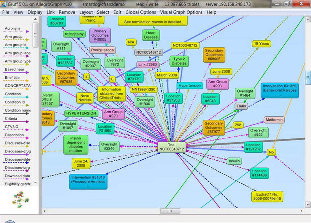
Figure 6-2. Visualizing a graph stored in AllegroGraph using Gruff [7]
The query view displays a view on which you can run a SPARQL or Prolog query and see the results in a table. The graphical query view makes it possible to plan a query visually as a diagram, by arranging the node boxes and link lines that represent triple patterns in the query. The triples patterns can contain variables as well as graph objects. The graphical query view supports hierarchies and filters and the automatic generation of SPARQL or Prolog queries. The table view displays a property table for a single node. Related nodes can be explored using hyperlinks, and property values can be edited directly. Each table row represents an RDF triple from the store.
Neo4j
Neo4j is one of the world’s leading graph databases, which queries connected data a thousand times faster than relational databases [8]. Neo4j has a free “Community Edition” and a commercial “Enterprise Edition,” both supporting property graphs; native graph storage and processing; ACID, a high-performance native API; its own graph query language, Cypher; and HTTPS (via plug-in). The advanced performance and scalability features that are available only in the Enterprise Edition are the Enterprise Lock Manager, a high-performance cache; clustering; hot backup; and advanced monitoring. Neo4j can be used as a triplestore or quadstore by installing an add-on called neo-rdf.
Installation
The Neo4j server is available in two formats under Windows: .exe and .zip. Neo4j can be installed using the .exe installer, as follows:
1. Download the latest Neo4j Server executable installation file from www.neo4j.org/download.
2. Double-click the .exe file.
3. Click Next and accept the agreement.
4. Start the Neo4j Server by clicking Neo4j Community under Start button ![]() All Programs
All Programs ![]() Neo4j Community
Neo4j Community ![]() Neo4j Community
Neo4j Community
By default, the C:\Users\username\Documents\Neo4j\default.graphdb database will be selected, which can be changed (see Figure 6-3).
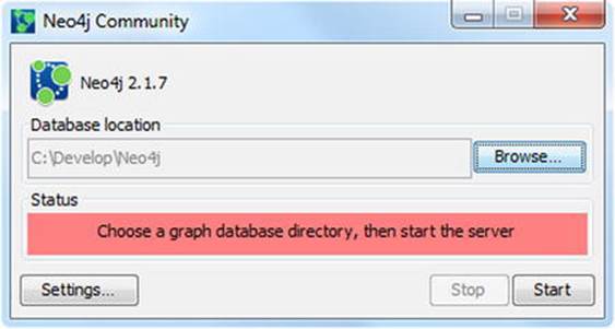
Figure 6-3. Neo4j ready to be started
5. Click the Start button, which creates the necessary files in the background in the specified directory.
6. Access Neo4j by visiting http://localhost:7474 in your browser (see Figure 6-4).
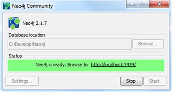
Figure 6-4. Neo4j started
The sidebar of the Neo4j web interface on the left provides convenient clickable access to information about the current Neo4j database (node labels, relationship types, and database location and size), saved scripts (see Figure 6-5), and information such as documentation, guides, a sample graph application, reference, as well as the Neo4j community resources.
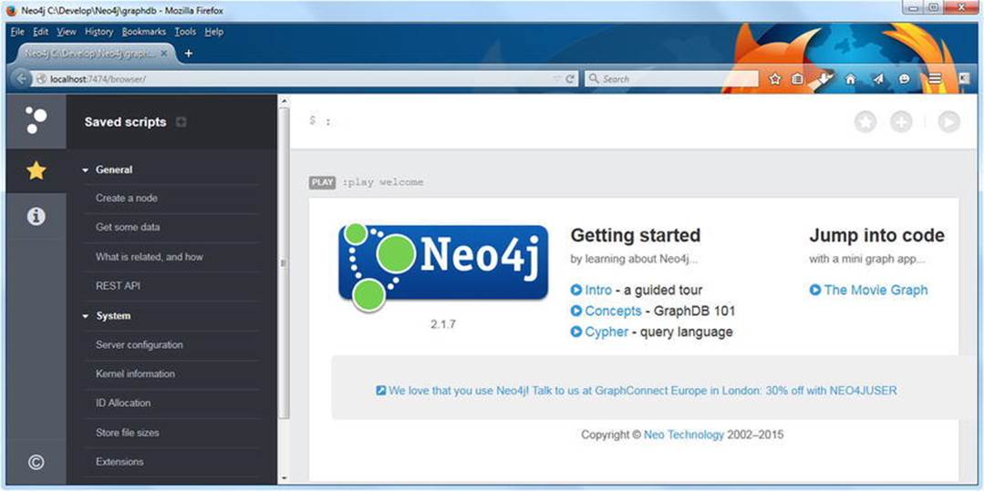
Figure 6-5. The web interface of Neo4j
The Neo4j web interface provides command editing and execution on the top (starting with $ :), including querying with Neo4j’s query language, Cypher. If you write complex queries or commands, or commands you want to use frequently, you can save them for future use. By default, the command editor is a single-line editor suitable for short queries or commands only. If you need more space, you can switch to multiline editing with Shift+Enter, so that you can write commands spanning on multiple lines or write multiple commands without executing them one by one (see Figure 6-6).
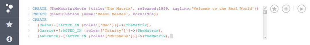
Figure 6-6. Writing Cypher commands
In multiline editing, you can run queries with Ctrl+Enter. Previously used commands can easily be retrieved using the command history. In the command line editor, you can use client-side commands as well, such as :help, which opens the Neo4j Help. The main part of the browser window displays the content, query answers, etc., depending on the commands you use. Each command execution results in a result frame (subwindow), which is added to the top of a stream to create a scrollable collection in reverse chronological order. Each subwindow can be maximized to full screen or closed with the two icons on the top right of the subwindow you hover your mouse over. Similar subwindows are used for data visualization as well. The stream can be cleared with the :clear command.
The web interface of Neo4j provides advanced visualization options. The nodes and relationships can be displayed with identifiers or labels in the color of your choice. The colors, line width, font size, and bubble size of graph visualizations can be changed arbitrarily through CSS style sheets, as shown in Figure 6-7.
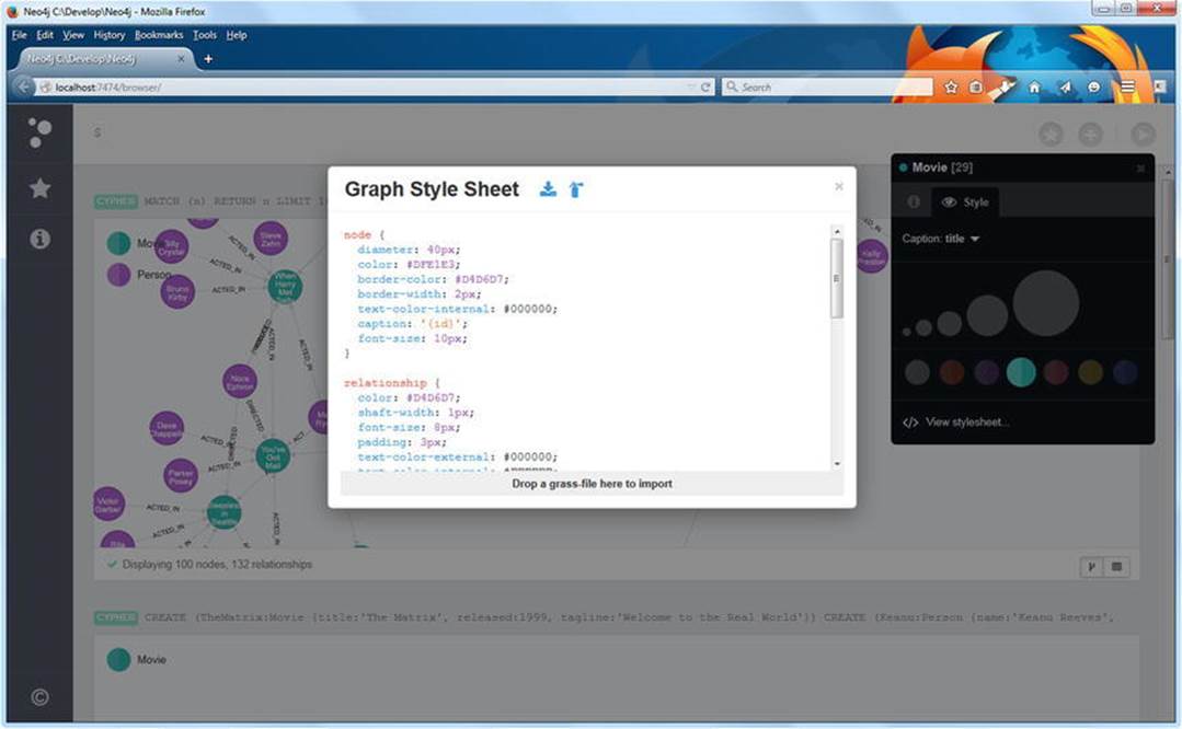
Figure 6-7. Graph visualization options in Neo4j
Java API
Neo4j has a Native Java API and a Cypher Java API. To demonstrate the native Java API of Neo4j, let’s develop a Java application in Eclipse.
1. If you don’t have Eclipse installed, follow the instructions discussed in Chapter 4.
2. Visit http://www.neo4j.org/download and under the Download Community Edition button, select Other Releases.
3. Under the latest release, select the binary of your choice for Linux or Windows.
4. Extract the archive.
5. In Eclipse, create a Java project by selecting File ![]() New
New ![]() Java Project.
Java Project.
6. Right-click the name of the newly created project and select Properties (or select File ![]() Properties).
Properties).
7. Select Java Build Path and click the Libraries tab.
8. Click Add Library… on the right.
9. Select User Library as the library type.
10.Click the Next ![]() button on the bottom.
button on the bottom.
11.Click User Libraries… on the right.
12.Click the New… button.
13.Add a name to your library, such as NEO4J_JAVA_LIB.
14.Click the Add external JARs… button on the right.
15.Browse to your Neo4j directory (neo4j-community-version_number) and go to the lib subdirectory.
16.Select all the .jar files (for example, with Ctrl+A) and click Open, which will add the files to your project library (see Figure 6-8).
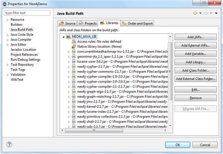
Figure 6-8. The Neo4j software library
17.Click OK.
18.Click Finish.
19.Once you click OK, the Neo4j software library will be added to your Eclipse project.
Let’s create a simple graph with nodes, a relationship between the nodes, node properties, and relationship properties.
1. Initialize the database as shown in Listing 6-24.
Listing 6-24. Initializing the Database
import org.neo4j.graphdb.GraphDatabaseService;
import org.neo4j.graphdb.Node;
import org.neo4j.graphdb.Relationship;
import org.neo4j.graphdb.RelationshipType;
import org.neo4j.graphdb.Transaction;
import org.neo4j.graphdb.factory.GraphDatabaseFactory;
public class Neo4jDemo
{
private static final String DB_PATH = "target/neo4jdemodb";
GraphDatabaseService graphDb;
Node firstNode;
Node secondNode;
Relationship relationship;
}
2. Define a new relationshSeip type as WEBSITE_OF (see Listing 6-25).
Listing 6-25. Defining a New Relationship Type
private static enum RelTypes implements RelationshipType
{
WEBSITE_OF
}
3. Create the main method, as shown in Listing 6-26.
Listing 6-26. Creating the main Method
public static void main(final String[] args)
{
Neo4jDemo dbsample = new Neo4jDemo();
dbsample.createDb();
dbsample.shutDown();
}
4. Create the graph nodes graphDb.createNode(); set node and relationship properties with setProperty; and display the RDF statement, using the label of the subject and the predicate, and the URI of the object (see Listing 6-27). The simple RDF statement will describe the relationship between the machine-readable description of a person and the URL of his/her web site.
Listing 6-27. Creating Nodes and Setting Properties
void createDb()
{
graphDb = new GraphDatabaseFactory().newEmbeddedDatabase(DB_PATH);
try ( Transaction tx = graphDb.beginTx() )
{
firstNode = graphDb.createNode();
firstNode.setProperty("uri", "http://dbpedia.org/resource/Leslie_Sikos");
firstNode.setProperty("label", "Leslie Sikos");
secondNode = graphDb.createNode();
secondNode.setProperty("uri", "http://www.lesliesikos.com");
secondNode.setProperty("label", "website address");
relationship = firstNode.createRelationshipTo(secondNode, RelTypes.WEBSITE_OF);
relationship.setProperty("uri", "http://schema.org/url");
relationship.setProperty("label", "website");
System.out.print(secondNode.getProperty("uri") + " is the ");
System.out.print(relationship.getProperty("label") + " of ");
System.out.print(firstNode.getProperty("label"));
tx.success();
}
}
5. Shut down the Neo4j database once you have finished (see Listing 6-28).
Listing 6-28. Shutting Down Neo4j
void shutDown()
{
System.out.println();
System.out.println("Shutting down database…");
graphDb.shutdown();
}
6. Run the application (see Listing 6-29) to display the RDF statement we created in the database (see Figure 6-9).
Listing 6-29. Final Code for Creating a Database with Nodes and Properties, and Displaying Stored Data
import org.neo4j.graphdb.GraphDatabaseService;
import org.neo4j.graphdb.Node;
import org.neo4j.graphdb.Relationship;
import org.neo4j.graphdb.RelationshipType;
import org.neo4j.graphdb.Transaction;
import org.neo4j.graphdb.factory.GraphDatabaseFactory;
public class Neo4jDemo
{
private static final String DB_PATH = "target/neo4jdemodb";
GraphDatabaseService graphDb;
Node firstNode;
Node secondNode;
Relationship relationship;
private static enum RelTypes implements RelationshipType
{
WEBSITE_OF
}
public static void main(final String[] args)
{
Neo4jDemo dbsample = new Neo4jDemo();
dbsample.createDb();
dbsample.shutDown();
}
void createDb()
{
graphDb = new GraphDatabaseFactory().newEmbeddedDatabase(DB_PATH);
try ( Transaction tx = graphDb.beginTx() )
{
firstNode = graphDb.createNode();
firstNode.setProperty("uri", "http://dbpedia.org/resource/Leslie_Sikos");
firstNode.setProperty("label", "Leslie Sikos");
secondNode = graphDb.createNode();
secondNode.setProperty("uri", "http://www.lesliesikos.com");
secondNode.setProperty("label", "website address");
relationship = firstNode.createRelationshipTo(secondNode, RelTypes.WEBSITE_OF);
relationship.setProperty("uri", "http://schema.org/url");
relationship.setProperty("label", "website");
System.out.print(secondNode.getProperty("uri") + " is the ");
System.out.print(relationship.getProperty("label") + " of ");
System.out.print(firstNode.getProperty("label"));
tx.success();
}
}
void shutDown()
{
System.out.println();
System.out.println("Shutting down database…");
graphDb.shutdown();
}
}
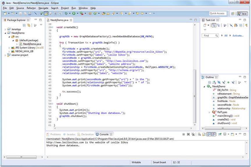
Figure 6-9. A Neo4j application in Eclipse
4Store
4Store is an efficient, scalable, and stable RDF database available for Linux systems such as Arch Linux, Debian, Ubuntu, Fedora, and CentOS, as well as Mac OS and FreeBSD [9]. To install 4Store on Linux, follow these steps:
1. Download the installer from http://www.4store.org.
2. Prepare your system to be used with 4Store by configuring it to look for libraries in /usr/local/lib and/or /usr/local/lib64. On most systems, you have to create a file called /etc/ld.so.conf.d/local.conf to achieve this, which contains these two paths, each on a separate line. You have to run /sbin/ldconfig as root. Once completed, the $PKG_CONFIG_PATH environmental variable should include the correct paths for locally installed packages.1 Check whether your Linux distribution includes all the dependencies, namely raptor, rasqal, glib2, libxml2, pcre, avahi, readline, ncurses, termcap, expat, and zlib.
3. Build your 4Store from Tarballs or Git. For the first option, extract the files from the .tar.gz archive with tar xvfz 4store-version.tar.gz. Change the working directory to the 4store-version directory with cd. Run ./configure, and then runmake. For the second option, change directory using cd to the directory that Git cloned, and run sh autogen.sh. The rest of the installation is the same as in the steps for the first option.
![]() Note Creating your build from Git might require additional dependencies.
Note Creating your build from Git might require additional dependencies.
4. Install 4Store by running make install as root.
If you want to install 4Store on a Mac, download the most recent version, open the .dmg, and install the 4Store application by dragging it into the Applications folder.
Once installed, you can run the 4Store application, which gives you a command line. You can create a triplestore using the command 4s-backend-setup triplestorename, start the triplestore using 4s-backend triplestorename, and run a SPARQL endpoint using 4s-httpd -p portnumber triplestorename. The web interface will be available in your browser at http://localhost:portnumber.
The simplest command to import data from an RDF file is to use 4s-import, specifying the database name to import the data to and the source RDF, as shown in Listing 6-30.
Listing 6-30. Importing Data from an RDF File to 4Store
4s-import your4store external.rdf
To import data programmatically, you can choose from a variety of options, depending on the language you prefer. In Ruby, for example, you can use 4store-ruby (https://github.com/moustaki/4store-ruby), a Ruby interface to 4Store working over HTTP. For accessing the SPARQL server, you need HTTP PUT calls only, which are supported by most modern programming languages without installing a store-specific package. Purpose-built software libraries, however, make the HTTP requests easier. In Ruby, for instance, you can use rest-client (https://github.com/rest-client/rest-client), as shown in Listing 6-31. If you don’t have rest-client installed, you can install it normally, e.g., sudo gem install rest-client.
Listing 6-31. Using rest-client
#!/usr/bin/env ruby
require 'rubygems'
require 'rest_client'
filename = '/social.rdf'
graph = 'http://yourgraph.com'
endpoint = 'http://localhost:8000'
response = RestClient.put endpoint + graph, File.read(filename), :content_type => ![]()
'application/rdf+xml'
puts "Response #{response.code}:
#{response.to_str}"
To run the script from the command line, use the ruby command with the filename as a parameter, such as ruby loadrdf24store.rb. Now, if you visit http://localhost:portnumber/status/size/ in your browser, the new triples added from the RDF file should be listed.
Let’s run a SPARQL query programmatically and process the results as XML, to list the RDF types of your dataset.
1. Install the XML parser Nokogiri for Ruby as gem install nokogiri.
2. Load all the required libraries (see Listing 6-32).
Listing 6-32. Loading Required Libraries
#!/usr/bin/env ruby
require 'rubygems'
require 'rest_client'
require 'nokogiri'
3. Create a string for storing the SPARQL query and another one to store the endpoint (see Listing 6-33).
Listing 6-33. Creating the Query and Endpoint Strings
query = 'SELECT DISTINCT ?type WHERE { ?thing a ?type . } ORDER BY ?type'
endpoint = 'http://localhost:8000/sparql/'
4. Using Nokogiri, process the XML output of the SPARQL query (see Listing 6-34).
Listing 6-34. Processing the SPARQL Query Output
response = RestClient.post endpoint, :query => query
xml = Nokogiri::XML(response.to_str)
5. Find all the RDF types in the XML output and display them with puts, as shown in Listing 6-35.
Listing 6-35. Finding the RDF Types of the Output
xml.xpath('//sparql:binding[@name = "type"]/sparql:uri', 'sparql' => 'http://www.w3.org/2005/sparql-results#').each do |type|
puts type.content
end
6. Save the script as a Ruby file and run it using the ruby command with the file name as the parameter, such as ruby rdf-types.rb.
Oracle
Oracle is an industry-leading database. Oracle Spatial and Graph, Oracle’s RDF triplestore/quadstore and ontology management platform, provides automatic partitioning and data compression, as well as high-performance parallel and direct path loading with the Oracle Database and loading through Jena [10].
Oracle Spatial and Graph supports parallel SPARQL and SQL querying and RDF graph update with SPARQL 1.1, SPARQL endpoint web services, SPARQL/Update, Java APIs with open source Apache Jena and Sesame, SQL queries with embedded SPARQL graph patterns, as well as SQL insert and update. It also supports ontology-assisted table data querying with SQL operators. Oracle Spatial and Graph features native inferencing with parallel, incremental, and secure operation for scalable reasoning with RDFS, OWL 2, SKOS, user-defined rules, and user-defined inference extensions. It has reasoned plug-ins for PelletDB and TrOWL. The semantic indexing of Oracle Spatial and Graph is suitable for text mining and entity analytics with integrated natural language processors. The database also supports R2RML direct mapping of relational data to RDF triples. For spatial RDF data storage and querying, Oracle supports GeoSPARQL as well.
Oracle Spatial and Graph can be integrated with the Apache Jena and Sesame application development environments, along with the leading Semantic Web tools for querying, visualization, and ontology management.
Blazegraph
Blazegraph is the flagship graph database product of SYSTAP, the vendor of the graph database previously known as Bigdata. It is a highly scalable, open source storage and computing platform [11]. Suitable for Big Data applications and selected for the Wikidata Query Service, Blazegraph is specifically designed to support big graphs, offering Semantic Web (RDF/SPARQL) and graph database (tinkerpop, blueprints, vertex-centric) APIs. The robust, scalable, fault-tolerant, enterprise-class storage and query features are combined with high availability, online backup, failover, and self-healing.
Blazegraph features an ultra-high performance RDF graph database that supports RDFS and OWL Lite reasoning, as well as SPARQL 1.1 querying. Designed for huge amounts of information, the Blazegraph RDF graph database can load 1 billion graph edges in less than an hour on a 15-node cluster. Blazegraph can be implemented in single machine mode (Journal), in high-availability replication cluster mode (HAJournalServer), or in horizontally sharded cluster mode (BlazegraphFederation). Blazegraph can execute distributed jobs by reading data not only from a local file system but also from the Web or the Hadoop Distributed File System (HDFS). The storage indexing is designed for very large datasets with up to 50 billion edges on a single machine, but Blazegraph can scale even larger graphs when implemented in a horizontally scaled architecture. Beyond high availability, the HAJournalServer also provides replication, online backup, and horizontal query scaling. BlazegraphFederation features fast, scalable parallel indexed storage and incremental cluster size growth. Both platforms support fully concurrent readers with snapshot isolation.
Blazegraph provides APIs for both Sesame and Blueprint. Blazegraph can be deployed as a server and accessed via a lightweight REST API. Blazegraph is released with Java wrappers, including a Sesame wrapper and a Blueprints wrapper. Blazegraph also has several enterprise deployment options, including a high-availability architecture and a dynamic-sharding scale-out architecture for very large graphs.
Summary
In this chapter, you learned about the power of graph databases and their advantages over mainstream relational and NoSQL databases. You now understand the concept of triples and quads, and the two main graph database types used for Semantic Web applications: the triplestores and the quadstores. You are now familiar with the most popular graph databases and know how to install and configure AllegroGraph, Neo4j, and 4Store and use their APIs for programmatic database access. You know the visualization options of AllegroGraph and Neo4j for displaying, analyzing, and manipulating graph nodes and links.
The next chapter will show you how to query structured datasets with SPARQL, the primary query language for RDF, and graph datastores, using proprietary query languages. You will learn how to write queries to answer complex questions based on the knowledge represented in Linking Open Data (LOD) datasets.
References
1. Cudré-Mauroux, P., Enchev, I., Fundatureanu, S., Groth, P., Haque, A., Harth, A., Keppmann, F. L., Miranker, D., Sequeda, J., Wylot, M. (2013) NoSQL Databases for RDF: An Empirical Evaluation. Lecture Notes in Computer Science 2013, 8219:310–325,http://dx.doi.org/10.1007/978-3-642-41338-4_20.
2. McColl, R., Ediger, D., Poovey, J., Campbell, D., Bader, D. A. (2014) A performance evaluation of open source graph databases. In: Proceedings of the first workshop on Parallel programming for analytics applications, pp 11–18, New York, NY,http://dx.doi.org/10.1145/2567634.2567638.
3. Heflin, J. (2015) SWAT Projects—the Lehigh University Benchmark (LUBM). http://swat.cse.lehigh.edu/projects/lubm/. Accessed 8 April 2015.
4. Franz, Inc. (2015) AllegroGraph RDFStore Web 3.0’s Database. http://franz.com/agraph/allegrograph/. Accessed 10 April 2015.
5. Franz, Inc. (2015) AllegroGraph Client Downloads. http://franz.com/agraph/downloads/clients. Accessed 10 April 2015.
6. Franz, Inc. (2015) Gruff: A Grapher-Based Triple-Store Browser for AllegroGraph. http://franz.com/agraph/gruff/. Accessed 10 April 2015.
7. Franz, Inc. (2015) http://franz.com/agraph/gruff/springview3.png. Accessed 10 April 2015.
8. Neo Technology Inc. (2015) Neo4j, the World’s Leading Graph Database. http://neo4j.com. Accessed 10 April 2015.
9. Garlik (2009) 4store—Scalable RDF storage. www.4store.org. Accessed 10 April 2015.
10. Oracle (2015) Oracle Spatial and Graph. www.oracle.com/technetwork/database/options/spatialandgraph/overview/index.html. Accessed 10 April 2015.
11. SYSTAP LLC (2015) Blazegraph. www.blazegraph.com/bigdata. Accessed 10 April 2015.
All materials on the site are licensed Creative Commons Attribution-Sharealike 3.0 Unported CC BY-SA 3.0 & GNU Free Documentation License (GFDL)
If you are the copyright holder of any material contained on our site and intend to remove it, please contact our site administrator for approval.
© 2016-2026 All site design rights belong to S.Y.A.