Neo4j in Action (2015)

Part 3. Neo4j in Production

Chapter 11. Neo4j in production

This chapter covers

· An overview of the high-level Neo4j architecture

· How to prepare for taking Neo4j to production

· How to scale and configure Neo4j to be highly available

· How to back up and restore your Neo4j database

This final chapter covers some of the more operational aspects involved in running Neo4j in a real production environment.

This includes looking at features such as running Neo4j in “High Availability” mode, paying particular attention to ensuring that Neo4j can operate in a fault-tolerant and scalable manner. It additionally covers how to back up and restore your database, for the scenarios where things have gone a little bit pear-shaped, as well as providing insight and instructions for how to configure important memory and cache settings, which play a large part in determining how well Neo4j performs.

To help you get the most out of this chapter, and indeed out of this book as a whole, this final chapter begins with a high-level tour through the Neo4j architecture, peeking under the hood in certain places. The primary purpose of this tour is to provide context, and a structured path for introducing and discussing operational and configurational aspects key to this chapter. It additionally provides us with a great opportunity to recap and reinforce some important and significant concepts covered in previous chapters along the way.

So, let’s begin!

11.1. High-level Neo4j architecture

As with any database, Neo4j has some configurations—knobs and levers that can be applied, pushed, or tweaked in order to direct or influence how the database operates and performs. We could provide a simple listing of what settings and options are available where, but we want you to get more out of this chapter than just knowing what you can change. Ideally, we want you to gain a little bit of mechanical sympathy for Neo4j—a basic feel for how Neo4j works under the covers. This will allow you to understand why certain setups, and the tweaking of certain settings, cause Neo4j to operate in the way it does, rather than just knowing that particular options exist.

Mechanical sympathy?

Mechanical sympathy is a metaphor that’s gaining in popularity in the computing world. It’s basically used to convey the idea that in order to get the most out of a tool or system properly (Neo4j in this case), it helps if you understand how it works under the covers (the mechanics). You can then use this knowledge in the most appropriate way.

The original metaphor itself is attributed to the Formula 1 racing car driver Jackie Stewart, who is believed to have said that in order to be a great driver, you must have mechanical sympathy for your racing car. Stewart believed that the best performances came as a result of the driver and car working together in perfect harmony.

Martin Thompson of LMAX fame was the first to popularize the use of this metaphor (as far as I’m aware) in the computing sense, when describing how the LMAX team came up with the low-latency, high-throughput disruptor pattern. His use of the metaphor can be seen in the presentation “LMAX—How to Do 100K TPS at Less than 1ms Latency” at www.infoq.com/presentations/LMAX.

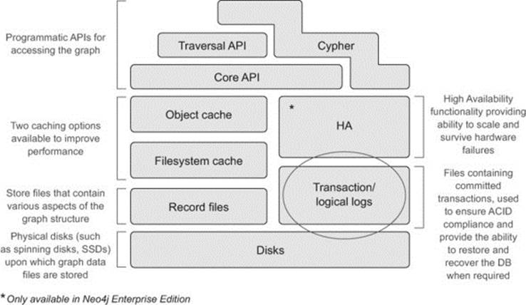
The high-level Neo4j architecture is shown in figure 11.1. Your tour through the architecture will begin at the bottom of this figure and wind its way up to the top.

Figure 11.1. High-level overview of the Neo4j architecture

Because this is an introductory book, we won’t be able to delve too deeply into all the aspects of Neo4j’s internals. Rather we aim to go just deep enough to help you appreciate and work in harmony with Neo4j, without getting too bogged down in low-level details. For a more in-depth treatment of the subject of how Neo4j works internally, see chapter 6, “Graph Database Internals” in Graph Databases by Jim Webber, Ian Robinson, and Emil Eifrem (O’Reilly, 2013). Although it’s a general-purpose graph database book, chapter 6 uses Neo4j’s architecture as an example to explain how a good, performant native graph database is laid out and implemented. Additionally, Tobias Lindaaker has done presentations on Neo4j internals, one of which, “An overview of Neo4j internals,” can be found here: www.slideshare.net/thobe/an-overview-of-neo4j-internals.

11.1.1. Setting the scene ...

The time has come for you to plan to put your application into production. From an operational perspective, there will typically be three main questions, or categories of questions, that will be asked of you regarding your new graph database:

· Physical storage —What kind and how much of it will be needed?

· Memory —How much memory (RAM) and CPUs are required to support efficient and performant running of the application and database?

· Scalability and redundancy —What’s required to ensure Neo4j can scale to accommodate a growing load, to ensure that it’s highly available (or available enough), and to ensure it can be properly backed up and restored in the event of failure?

Working backward, recovery and backups are covered in section 11.3, HA is covered in section 11.2, and the memory- and CPU-related questions in section 11.1.4. First up, we’ll tackle the question of storage and disks, which leads us neatly to our starting point at the bottom of Neo4j’s architectural stack.

11.1.2. Disks

At the bottom of the architectural stack are the physical disks where Neo4j actually stores the graph data.

What kind of disks should be used?

Neo4j doesn’t dictate what kind of disks should be used, but it goes without saying that faster disks will lead to faster performance whenever physical disk IO is required. Making use of disks that provide lower seek times (such as solid state drives, a.k.a. SSDs) will generally provide a read-performance boost of 10 to 20 times that of traditional spinning disks.

As you’ll learn in section 11.1.4, you should aim to keep as much of the graph in memory as possible, as this reduces disk IO, which helps enable Neo4j to perform at its best. At some point, however, your application or database will need to go to disk to read data. At the very least, this will occur when you initially start up your database and begin to access cold parts of the graph. It may also occur if your graph is simply too big to fit into memory (see section 11.2.4 on cache sharding).

Avoiding disk IO is one of the key factors in maximizing Neo4j performance, and having speedy disks for the times when this IO can’t be avoided can make quite a difference.

How much space do i need for my graph database?

The amount of space required obviously depends on how much data you plan on storing in Neo4j, and on any additional space required to support the runtime operation of Neo4j.

All Neo4j data lives under a single, top-level Neo4j directory (by default, data/graph.db in a server-based setup). This includes the core graph data, which lives in a set of store files (covered in section 11.1.3), transaction logs (covered in section 11.1.5), and the rest (including things like indexes and other minor files) in other files.

All of the main store files that contain the core graph structure are consistent in the amount of space they occupy—they have fixed record sizes, which can help you estimate the ultimate file sizes. This helps greatly in calculating what the core database sizing requirements are, although this alone isn’t always enough to work it out exactly. This is partly due to the fact that Neo4j itself will sometimes create additional files as part of its internal runtime optimizations, which can’t necessarily be anticipated upfront. Indexes and labels will also take up more space.

You can do rough math based on your estimates of the number of nodes, relationships, and properties required. The general formula for calculating the space required for the core graph data is

Core Graph Size (in bytes) =

(num nodes X node store record size in bytes) +

(num relationships X relationship store record size in bytes) +

(num properties X average bytes per property)

The fixed record sizes are discussed in more detail in the next section, but at the time of writing, the node store uses 14 bytes and the relationship store uses 33 bytes. Remember that there will be additional disk storage requirements for indexes, transaction logs, and the like, and these should also be taken into account when calculating the total amount of disk space required. Having said that, calculating the core graph data size, which is usually what takes up much of the disk space used by Neo4j, is relatively straightforward.

Neo4j hardware sizing calculator

Neo Technology provides an online hardware sizing calculator to provide rough estimates for the minimum hardware configuration required, given a certain set of inputs, such as the expected number of nodes, relationships, properties, number of users, and so on. This calculator deals not only with disk storage capacity, but also RAM and clustering setup recommendations.

It should be stressed that this calculator is only meant to provide a rough estimate. If you’re embarking on a mission-critical project, you’re advised to seek a more accurate assessment from qualified engineers, which can take many other factors into consideration. But for a rough and ready starting calculation, this calculator will generally serve just fine.

You can find the hardware sizing calculator on the Neo Technology site, www.neotechnology.com/hardware-sizing.

11.1.3. Store files

Neo4j stores various parts of the graph structure in a set of files known as store files. These store files are generally broken down by record type—there are separate files for nodes, relationships, properties, labels, and so on. The structure and layout of the data in these files has specifically been designed and optimized to provide an efficient storage format that the Neo4j runtime engine can exploit to provide very performant lookups and traversals through the graph. One of the core enablers is the fact that Neo4j stores data according to the index-free adjacency principle.

The index-free adjacency what?

The index-free adjacency principle (or property) is a fancy term that refers to graph databases that are able to store their data in a very particular way. Specifically, each node stored within the database must have a direct link or reference to its adjacent nodes (those nodes directly connected to it) and must not need to make use of any additional helper structures (such as an index) to find them.

By storing its data in this manner, Neo4j is able to follow pointers directly to connected nodes and relationships when performing traversals, making this type of access extremely fast compared to non-index-free adjacency stores, such as the traditional relational database. In Neo4j there’s no overhead incurred when trying to locate immediately connected nodes; non-index-free adjacency stores would first need to use a supporting (index) structure to look up which nodes were connected in the first place. Only then would they be able to go off and access the nodes. Index-free adjacency allows for query times that are proportional to how much of the graph you search through, rather than to the overall size of the graph.

Recall the football stadium analogy from the sidebar in chapter 1—“What is the secret of Neo4j’s speed?”

Imagine yourself cheering on your team at a small local football stadium. If someone asks you how many people are sitting 15 feet around you, you’ll get up and count them—you’ll count people around you as fast as you can count. Now imagine you’re attending the game at the national stadium, with a lot more spectators, and you want to answer the same question—how many people are there within 15 feet of you. Given that the density of people in both stadiums is the same, you’ll have approximately the same number of people to count, taking a very similar time. We can say that regardless of how many people can fit into the stadium, you’ll be able to count the people around you at a predictable speed; you’re only interested in the people sitting 15 feet around you, so you won’t be worried about packed seats on the other end of the stadium, for example.

This analogy provides a practical demonstration of how a human would naturally employ the index-free adjacency principle to perform the counting task.

Store files are located under the main graph database directory (by default, data/graph.db in a server setup) and are prefixed with neostore. Table 11.1 shows the main store files used by Neo4j, as well as some of their key properties.

Table 11.1. Primary store files in use and their associated properties

^* Block size can be configured with the string_block_size and array_block_size parameters. Default block size is 120 bytes with 8 bytes for overhead.

The main store files have a fixed or uniform record size (14 bytes for nodes, 33 bytes for relationships, and so on). Besides playing an important part in enabling fast lookups and traversals, the fixed length makes calculations about how much space and memory to allocate for your graph a little easier to reason about and plan for, as mentioned in section 11.1.2.

The node and relationship store files simply store pointers to other nodes, relationships, and property records, and thus fit neatly into fixed record sizes. Properties, on the other hand, are slightly harder to deal with because the actual data that they represent can be of variable length. Strings and arrays, in particular, will have variable length data in them, and for this reason they’re treated specially by Neo4j, which stores this dynamic type of data in one or more string or array property blocks. For more information, refer to the Neo4j Manual (http://docs.neo4j.org/chunked/stable/configuration-caches.html). The details are scattered throughout subsections of the manual, currently sections 22.6, 22.9, and 22.10.

How do fixed-length records improve performance?

The use of fixed-length records means that lookups based on node or relationship IDs don’t require any searching through the store file itself. Rather, given a node or relationship ID, the starting point for where the data is stored within the file can be computed directly. All node records within the node store are 14 bytes in length (at the time of writing). IDs for nodes and relationships are numerical and are directly correlated to their location within a store file. Node ID 1 will be the first record in the node store file, and the node with ID 1000 will be the thousandth.

If you wanted to look up the data associated with node ID 1000, you’d be able to calculate that this data would start 14000 bytes into the node store file (14 bytes for each record x node ID 1000). The complexity involved in computing the starting location for the data is much less (O(1) in big O notation) than having to perform a search, which in a typical implementation could cost O(log n). If big O notation scares you, fear not; all you really need to understand here is that it’s generally much faster to compute a start point than it is to search for it. When a lot of data is involved, this can often translate into significant performance gains.

The fixed record size also plays an important part in providing a quick mechanism for calculating where in the file a contiguous block of records is stored; this is used by the filesystem cache (see section 11.1.4) to load portions of the store files into cache.

There are two key features that you should be aware of when it comes to the store file structure.

The first is that these fixed record sizes can be used to help estimate the amount of space that the core graph files will take up on disk, and thus how big your disks may need to be (see section 11.1.2).

The second is that these store records have a direct 1:1 mapping when it comes to the filesystem cache and how it works. Caching is covered in the next section, but basically, the filesystem cache is responsible for loading portions of the store files into available RAM for fast access. Paying close attention to the size of these store file records is an important factor in being able to calculate what your memory and caching requirements may be.

11.1.4. Neo4j caches

Even with super-fast disks and Neo4j’s efficient storage structure, a latency penalty will always be incurred whenever processing requires a trip from the CPU to disk. This latency penalty can be dramatically reduced if the data to be accessed can be held in memory (RAM of some sort) where disk IO is reduced or even eliminated. Neo4j operates optimally when data is cached in memory.

So what does in memory mean, as far as Neo4j is concerned? Neo4j makes use of a two-tiered caching strategy: the filesystem cache and object cache. These caches, as well as where they live within the overall memory of a single server, are illustrated in figure 11.2.

Figure 11.2. Neo4j’s use of RAM for caching

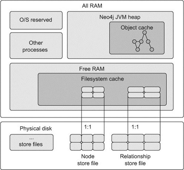
Filesystem cache

The filesystem cache is an area of free RAM (RAM that hasn’t yet been allocated to any process) that the OS sets aside to help speed up reading from and writing to files. The filesystem cache makes use of something called memory-mapped IO. Whenever a process requests a file, the filesystem cache is checked to see if it has already been loaded there. If not, the physical file (or part of the file requested) is read from disk into this memory area. Subsequent requests for the same file (or a portion of the file) can then be served from memory, dramatically increasing performance by eliminating the need for physical disk IO. Changes to the data are also written to the filesystem cache, rather than immediately to the physical disk. The performance lift gained from accessing a file through the filesystem cache, rather than going to a spinning disk, is around 500 times faster.

The OS is in charge of managing this memory, including making decisions about when to flush changes written to this memory area down to the physical disk. Although the OS has the final say as to when data is read into and written from this area, processes can request certain files, or portions of files, to be loaded into this memory area for processing.

Neo4j takes advantage of this OS feature (through the Java NIO packages) to efficiently load, read, and write to and from the store files. This provides the first level (sometimes called the low-level) caching functionality within Neo4j.

What happens if the system crashes and the data has only been written to memory and not to disk?

If the OS is in control of when data is flushed to disk for the filesystem cache, what happens to that data in the event of a system failure?

In short, data held in this memory area is lost. Fear not, however, as Neo4j makes use of a separate, durable, transaction log to ensure that all transactions are physically written to a file that is flushed to disk upon every commit. Whenever a commit happens, although the store files themselves may not yet have physically been updated, the transaction log will always have the data on disk. The transaction log (covered in section 11.1.5) can then be used to recover and restore the system when starting up after a failure. In other words, this transaction log can be used to reconstruct the store files so that they fully reflect what the system looked like at the point of the last commit, and thus what the store files would have looked like had the data been flushed to disk before the crash.

Configuring the filesystem cache

Ideally, you should aim to load as much of your persistent graph data (as stored within the physical store files on disk) into memory as possible. You can control what parts, and how much, of the persistent graph you want loaded into memory. In practice, as all graph data lives in the store files, this generally involves looking at how much space these files occupy on disk (or how large you expect them to become), and trying to reserve an appropriate amount of RAM for each one.

Suppose you have a top-level Neo4j database directory that occupies approximately 2.2 GB of data, made up of the following store files and sizes:

20M neostore.nodestore.db

60M neostore.propertystore.db

1.2G neostore.propertystore.db.strings

900M neostore.relationshipstore.db

The following snippet shows a configuration that will ensure that the whole of the graph can fit into the memory allocated to the filesystem cache. The settings shown in this configuration file reserve approximately 2.5 GB of RAM, which allows for about 10% data growth:

neostore.nodestore.db.mapped_memory=22M

neostore.propertystore.db.mapped_memory=66M

neostore.propertystore.db.strings.mapped_memory=1.4G

neostore.relationshipstore.db.mapped_memory=1.0G

neostore.propertystore.db.arrays.mapped_memory=0M

When running Neo4j in server mode, these settings are specified in the neo4j.properties file found under the conf directory.

For an embedded setup, the configuration settings can be passed in when the graph database is constructed, either via a reference to a neo4j.properties file, accessible from somewhere on the classpath, or directly within Java via a Map.

You’ll have noticed that there’s a 1:1 mapping between the configuration settings and the physical store files on disk. Within the broader filesystem cache memory area, Neo4j ensures that separate, individual file buffer caches are maintained for each store file, and thus allows cache configuration on a per store basis as well. This makes it is possible to configure how much of each store file should be loaded into RAM independently of one another.

Different applications will have different usage patterns, and being able to independently tune these cache areas enables you to ensure that the app can perform as well as possible, especially if there isn’t enough free RAM available to load the whole graph into memory.

Note

When we cover HA, we’ll also look at the concept of cache sharding, which can be used to help load appropriate portions of the graph into memory across multiple machines.

Specific scenarios and configuration examples for the memory-mapped IO caches are provided in the “Memory mapped IO settings” section of the official Neo4j Manual at http://docs.neo4j.org/chunked/stable/configuration-io-examples.html.

Default configuration

In the absence of any configuration from the user, Neo4j will try to work out what it thinks is best, given its knowledge of the system and the amount of RAM available to it.

Object cache

The filesystem cache goes a long way to improving performance by reducing disk IO, but Neo4j is a JVM-based application that deals with the concepts of nodes and relationships (stored as Java objects) rather than only interacting with raw files.

Neo4j’s object cache is an area within the JVM heap where Neo4j stores the Java object versions of nodes and relationships in a form that’s optimized for use in traversals and quick retrievals by the core Neo4j APIs.

The previous section showed you how utilizing the filesystem cache could provide a performance boost of up to 500 times compared to accessing the same data on a spinning disk. The object cache allows for yet another performance boost over and above the filesystem cache. Accessing data from within the object cache (as opposed to going to the filesystem cache) is about 5,000 times faster!

Configuring the object cache

There are two aspects to configuring the object cache. The first involves configuring the JVM, and specifically the JVM heap, which is done by providing an appropriate -Xmx???m parameter to the JVM upon startup. The second is choosing an appropriate cache type, which is controlled by setting the cache_type parameter in the neo4j.properties file.

We’ll tackle the JVM configuration first, as this can have a massive impact on the performance of your application and database. The general rule of thumb is that the larger the heap size the better, because this means a larger cache for holding and processing more objects, and thus better performance from the application. This statement holds true for the most part, but it’s not always that simple.

One of the attractive features of JVM-based development is that, as a developer, you don’t need to worry about allocating and deallocating memory for your objects (as you’d need to in other languages like C++). This is instead handled dynamically by the JVM, which takes responsibility for allocating storage for your objects as appropriate, as well as cleaning up unreferenced objects via the use of a garbage collector. Garbage collectors can be tuned and configured, but in general, heap sizes larger than 8 GB seem to cause problems for quite a few JVMs.

Large heap sizes can result in long GC pauses and thrashing—these are exactly the types of wasteful scenarios you want to avoid. Long GC pauses and thrashing are horrendously detrimental to performance, because the JVM ends up spending more time trying to perform the maintenance activities of cleaning up and freeing objects than it does enabling the application to perform any useful work.

So how much memory should be allocated to the JVM for Neo4j to operate optimally? This is one of those areas where you may need to play around a bit until you can find a sweet spot that makes use of as much of the JVM heap space as possible without causing too many GC-related problems. Configuring the JVM with the following startup parameters and values provides a good starting point:

· Allocate as much memory as possible to the JVM heap (taking into account your machine and JVM-specific limits—6 GB or less for most people). Pass this in via the -Xmx???m parameter.

· Start the JVM with the -server flag.

· Configure the JVM to use the Concurrent Mark and Sweep Compactor garbage collector instead of the default one, using the -XX:+UseConcMarkSweepGC argument.

For a more detailed discussion about JVM- and GC-based performance optimizations within Neo4j, consult the official documentation at http://docs.neo4j.org/chunked/stable/configuration-jvm.html.

Construct a sample graph early on to help determine memory (and disk) requirements

There’s generally no foolproof and completely accurate way to calculate exactly how much heap space the JVM will require to hold and process your graph in memory. What many people choose to do is construct a small, but relatively accurate (if possible) representation of their graph as early on in the development process as possible. Even though this sample graph may change as time goes on, it can be used to help work out how much space and memory might be required for a larger dataset with a similar structure and access patterns.

This is useful for working out appropriate settings for the filesystem cache, object cache, and general storage requirements.

The second configuration is the cache_type parameter in the neo4j.properties file. This controls how node and relationship objects are cached. For the purposes of brevity, we’ll list the options available with the brief descriptions specified in the official documentation; this can be seen intable 11.2. For more information see the “Caches in Neo4j” section of the Neo4j Manual at http://docs.neo4j.org/chunked/stable/configuration-caches.html.

Table 11.2. Object cache-type options as per the official documentation

^* Default cache_type

^** Only available in Neo4j Enterprise edition. (Note: this cache has successfully been used by some customers with heap sizes of up to 200 GB.)

As increasing the JVM heap size eats into the overall RAM available on the box, the setting of the heap size and the settings for the filesystem cache should really be considered together. Remember to include other factors as well, such as the OS’s requirements for RAM and any other processes that may be running on the box. If you’re running in embedded mode, the Neo4j database will be sharing the JVM heap with your host application, so ensure that this is catered to as well!

Caching summary

Your caching approach can be summarized as follows:

· At a minimum, aim for a setup that allows for all, or as much as possible, of the graph to fit into the filesystem cache.

· Thereafter, make as much use of the object cache as feasible.

11.1.5. Transaction logs and recoverability

Shifting to the right side of our high-level architecture diagram (see figure 11.3), we’ll focus on providing a brief overview of how the transaction log files (sometimes also referred to as the logical files), are used to ensure Neo4j is ACID-compliant. But more importantly for this chapter, we’ll look at how the transaction logs are used to promote self-healing and recoverability.

Figure 11.3. Recap of where transaction logs fit into the overall Neo4j architecture

In chapter 7 you learned that Neo4j is a fully ACID-compliant (atomic, consistent, isolated, durable) database. Many ACID-based systems (Neo4j included) use what’s known as a write-ahead log (WAL) as the mechanism for providing the atomicity and durability aspects of ACID. The use of a WAL means that whenever a transaction is committed, all changes are written (and physically flushed) to the active transaction log file on disk before they’re applied to the store files themselves. Recall that the use of the filesystem cache means that writes to the store files may still only be in memory—the OS is in charge of deciding when to flush these areas to disk. But even if the system crashes and committed changes haven’t been applied to the physical store files, the store files can be restored using these transaction logs.

All transaction log files can be found in the top level of the Neo4j database directory and they follow the naming format nioneo_logical.log.*.

Behind the scenes—recovering from an unclean shutdown

Unclean shutdown usually refers to the scenario where a Neo4j instance has crashed unexpectedly. It can also refer to situations where Neo4j was intentionally shut down, but the key point is that Neo4j was not allowed to perform its usual cleanup activities for whatever reason. When an unclean shutdown occurs, the following warning message can generally be seen in the logs the next time the database is started up—non clean shutdown detected.

When Neo4j starts up, the first thing it will do is consult the most recent transaction log and replay all of the transactions found against the actual store files. There’s a possibility that these transactions will already have been applied to the store (remember that the OS controls when the filesystem cache is flushed to disk—this may or may not have happened). Replaying these transaction again isn’t a problem, however, as these actions are deemed to be idempotent—the changes can be applied multiple times without resulting in a different result in the graph.

Once the Neo4j instance has started up, its store files will have been fully recovered and contain all the transactions up to and including the last commit—and you’re ready to continue!

Besides aiding with transactions and recoverability, the transaction log also serves as the basis upon which the HA functionality is built—the ability to run Neo4j in a clustered setup.

11.1.6. Programmatic APIs

At the very top of the Neo4j architectural stack are the three primary APIs (Cypher, Traversal, and Core), which are used to access and manipulate data within Neo4j (see figure 11.1). Previous chapters have covered these APIs in-depth so we won’t be covering that ground again.

Technically, there isn’t any operational aspect to these APIs; there are no specific settings to tune these APIs in the same way as, for example, the caches. They do form part of the overall Neo4j architecture that you’re touring, so they get a special mention here.

The only thing we want to highlight in this section is that, although each of these APIs can be used individually to interact with the graph, they build on each other to a certain extent (in a bit of a stack-like manner). More importantly, they each have their own sweet spots. Depending on what you’re trying to do, it’s up to you to choose the right tool for the job. Figure 11.4 provides an overview of the primary goals and approaches used by each API.

Figure 11.4. Programmatic API stack

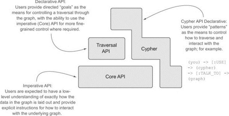
If performance is of the utmost importance, you’ll probably want to drop down and use the Core API, as this provides you with the most flexibility and control over your interaction with the graph. This comes at a price, as it requires explicit knowledge of exactly how the graph data is laid out in order to interact with it, and this interaction can be quite verbose.

The Traversal API provides a slightly more friendly API, where users provide goals such as “do a depth-first search to depth 3,” allowing Neo4j to take care of interacting with the core API to realize the results. Although this API is easier for the developer to use, the slightly higher level of abstraction means that it may not perform quite as optimally as the Core API.

Then there’s Cypher—the declarative, humane, graph query language, and arguably the most intuitive and friendly of all the APIs to use. Many would say Cypher represents the future of Neo4j, as so much development effort is being directed in this area. Its general appeal and ease of use and understanding (aimed at developers and operational staff alike) has made it a very compelling part of Neo4j’s product surface. At present, Cypher can’t match the performance of the core API in most cases. In Neo4j 1.x, Cypher binds to the Core and Traversal APIs (so it can never do any better than those APIs), but in the future (especially from Neo4j 2.0 onward) Cypher will bind lower in the stack to a sympathetic API that will support query optimization and other runtime efficiencies. Although Cypher can’t match the Core API today for performance, there’s no reason to think it won’t be on par, or even outperform the Core API in the future—time will tell.

11.2. Neo4j High Availability (HA)

The Enterprise edition of Neo4j comes with a Neo4j HA component that provides the ability for Neo4j to run in a clustered setup, allowing you to distribute your database across multiple machines. Neo4j makes use of a master-slave replication architecture and, broadly speaking, provides support for two key features: resilience and fault tolerance in the event of hardware failure, and the ability to scale Neo4j for read-intensive scenarios.

HA versus clustering

You’ll often hear the terms HA and cluster used interchangeably when referring to a multimachine setup within Neo4j. In essence, these are referring to the same concepts but with different names.

Resilience and fault tolerance refer to the ability of Neo4j to continue functioning and serving clients even in the presence of network disruptions or hardware failures. If one of the machines in your cluster blows up, or a link to your network dies, Neo4j should be able to continue without a total loss of service.

Besides being able to handle hardware failure scenarios reliably, the master-slave architecture has the added benefit of providing a way to scale Neo4j horizontally for read-mostly scenarios. In this context, read-mostly scenarios can refer to applications with high throughput requirements where there’s a need, or desire, to scale reads horizontally across multiple slave instances. It’s additionally used to support caching sharding (discussed in section 11.2.4), which enables Neo4j to handle a larger read load than could otherwise be handled by a single Neo4j instance.

11.2.1. Neo4j clustering overview

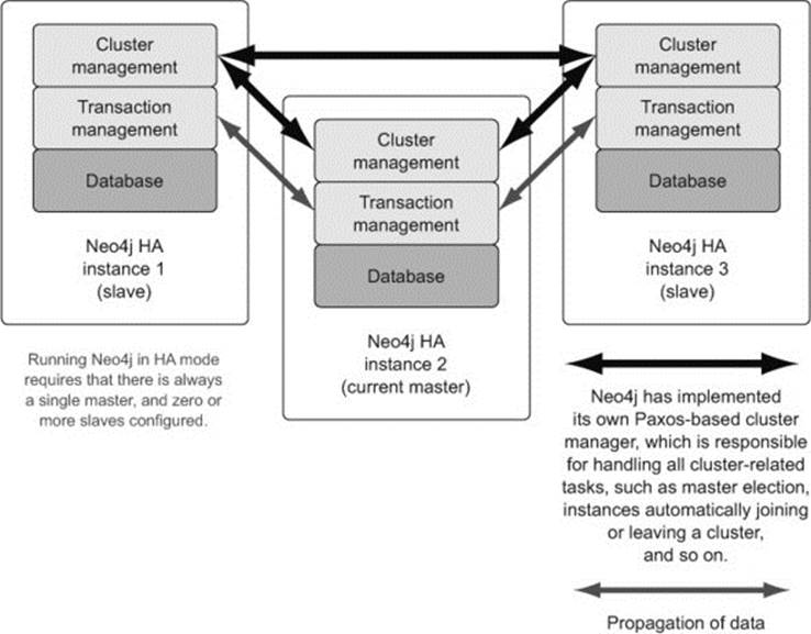
A Neo4j HA cluster involves a set of Neo4j Enterprise instances that have all been configured to belong to a single logical unit (cluster). At any given time, it’s expected that there will always be a single master present, with zero or more slaves configured as required.

Neo4j’s HA architecture has recently undergone a bit of an overhaul in an effort to simplify the setup and operational running requirements. Prior to Neo4 1.9, Neo4j used Apache ZooKeeper (http://zookeeper.apache.org) to provide the cluster coordination functionality. Although ZooKeeper is a fine product, its use within the Neo4j architecture posed a number of problems, including having to deal with the additional operational overhead, setup, and integration of a separate coordinator component. It also had restrictions in terms of being able to dynamically reconfigure itself; for some cloud-based setups, this proved somewhat restrictive.

For these, as well as some other reasons, Neo Technology decided to roll its own cluster-coordination mechanism, and from Neo4j version 1.9 onward, including Neo4j 2.0, ZooKeeper is no longer used. The Neo4j implementation is based on the Paxos protocol, which primarily handles master election, but Neo4j also takes responsibility for the handling of all general cluster-based management tasks. It’s not necessary to understand the finer details of the Paxos protocol (that’s well beyond the scope of this book), but if you’re interested, Leslie Lamport’s article, “Paxos Made Simple” (2001), provides a simple introduction to the subject: www.cs.utexas.edu/users/lorenzo/corsi/cs380d/past/03F/notes/paxos-simple.pdf.

Figure 11.5 shows the key workings of the new Neo4j cluster coordination mechanism based on the Paxos protocol.

Figure 11.5. Sample Neo4j HA cluster setup with 1 master and 2 slaves

Within a Neo4j HA cluster, each database instance is self-sufficient when it comes to the logic required to coordinate and communicate with other members of the cluster. When an HA database instance starts up, the first thing it will try to do is establish a connection to its configured cluster. The neo4j.properties file contains the various properties controlling the HA configuration (all prefixed with ha*), including the property listing the initial set of other members belonging to the cluster—ha.initial_hosts).

If the cluster doesn’t exist upon startup, meaning this is the first machine to attempt a connection to the cluster, then this process will take care of establishing the initial cluster, installing this instance as the master.

All write requests are ultimately performed through the master, although it’s possible to send the request to a slave. Doing so, however, is significantly slower than going directly to the master. In this scenario, the slave has logic built into it to synchronously ensure the write is first performed on the master, and then applied to itself as well.

Changes are propagated back out of slaves through a configurable push- and/or pull-based mechanism.

What about CAP and ACID?

Running in a clustered setup has some implications for the ACID guarantee provided by Neo4j. Neo4j’s single-machine consistency guarantee loosens to become eventually consistent in a cluster. What does that mean?

A NoSQL book isn’t complete without some mention of, or reference to, the CAP theorem. Neo4j claims to be an ACID-compliant database, and when running on a single machine, this guarantee is absolute. As soon as you introduce the ability for your database to be partitioned across a network, however (through the master-slave setup), the perfect ACID guarantee (at least the availability and consistency aspects) needs to be loosened or somewhat redefined.

An example always helps to clarify things, so let’s pretend that your database has now been spread (replicated) across three instances, and you update a node on one (the master) of them. What happens to the slaves? When one of them tries to read this data, will it see this update straight away (will all the slaves be able to see a consistent view of the data at all times), or will there be any periods where it’s slightly out of date? If there’s a network failure, can you still read and write through any machine, including the slaves?

For the purposes of this discussion, the CAP theorem, originally proposed by Eric Brewer in 2000, with his own subsequent retrospective update posted 12 years later,^[1] implies that you can’t have both consistency and availability 100% of the time when partitions are involved—there needs to be a trade-off of some sort.

¹ Eric Brewer, “CAP Twelve Years Later: How the ‘Rules’ Have Changed” (2012), www.infoq.com/articles/cap-twelve-years-later-how-the-rules-have-changed.

Neo4j is an AP database, which means it’s eventually unavailable in the presence of partitions (it becomes read-only for safety reasons if the network is extremely fragmented). Slaves will become eventually consistent by having updates either pushed to, or pulled by, them over some period of time. These values are configurable, so the inconsistency window can be controlled as each application or setup dictates. We’ll discuss this more in section 11.2.3.

Before we dive into more specifics around how certain HA features work within Neo4j, we’ll go through an exercise of setting up a three-machine cluster. This allows you to get your hands dirty, so that you can then play and experiment with some of the setup options as we discuss them in this chapter.

Switching from a single machine setup to a clustered setup

For clients currently making use of an existing single-machine (embedded or server) setup, switching to a clustered environment should be a relatively straightforward and pain-free affair. This is possible because Neo4j HA was designed from the outset to make such a transition as easy as possible. There will obviously be additional configuration involved in order to ensure the server can establish itself as a member of a cluster (we’ll be covering this shortly), but from the client’s perspective, the operations available and the general way in which the interaction with the server is undertaken should remain largely unchanged.

Embedded mode

For embedded clients, the Neo4j JAR dependencies will need to be changed from the Community to the Enterprise edition, if this hasn’t already been done. The only change required thereafter is in the way the GraphDatabaseService instance is created. Instead of using theGraphDatabaseFactory to create the GraphDatabaseService, a HighlyAvailableGraphDatabaseFactory should be used. As both of these factories generate implementations that make use of the same (GraphDatabaseService) interface, there are no additional changes required for any clients using it.

The following code snippet shows this code in action, with the HA-specific changes highlighted:

graphDatabaseService = new HighlyAvailableGraphDatabaseFactory()

.newHighlyAvailableDatabaseBuilder("/machineA")

.loadPropertiesFromFile(machineAFilename)

.newGraphDatabase();

Server mode

Single server instances that are not currently running against the Enterprise edition will first need to be upgraded to the Enterprise edition. Then it’s simply a case of configuring the server to be part of an appropriate cluster.

11.2.2. Setting up a Neo4j cluster

Let’s go through the process of setting up a three-machine, server-based cluster. Neo4j HA works just as well for embedded instances. As this is primarily going to be used for demo purposes, we’ll run all three instances on the same machine; but in production you’d more than likely run different instances on different machines.

Note

These instructions are for *nix environments (the actual examples were done on OS X 10.9.2), but an equivalent process can be followed for a Windows setup. We ran this HA setup against Neo4j version 2.0.2.

Initial setup

Follow these steps to perform the initial setup:

1. Create a base parent directory, such as ~/n4jia/clusterexample.

2. Download the Enterprise version of Neo4j and unpack the zip file (for Windows) or tar file (for Unix) into this folder. On the Mac, this would look like the following:

~/n4jia/clusterexample/neo4j-enterprise-2.0.2

3. Rename this folder machine01, and duplicate the directory, along with all of its content, into directories machine02 and machine03. Your resulting file structure should look like this:

~/n4jia/clusterexample/machine01
~/n4jia/clusterexample/machine02
~/n4jia/clusterexample/machine03

4.

Within each machine’s base directory, locate the conf/neo4j-server.properties file and ensure the following properties are set:

5.

Within each machine’s base directory, locate the conf/neo4j.properties file and ensure that the following properties are set:

Startup and verify

Follow these steps to start up and verify your servers:

1. Startup the servers in each directory by issuing the start command as shown below:

~/n4jia/clusterexample/machine01)$ bin/neo4j start
~/n4jia/clusterexample/machine02)$ bin/neo4j start
~/n4jia/clusterexample/machine03)$ bin/neo4j start

2. Visit the Web Admin Console (see appendix A) on a browser for each server once you have given it a bit of time to start up to verify that it started correctly and explore the details provided:

http://127.0.0.1:7471/webadmin/#/info/org.neo4j/High%20Availability/
http://127.0.0.1:7472/webadmin/#/info/org.neo4j/High%20Availability/
http://127.0.0.1:7473/webadmin/#/info/org.neo4j/High%20Availability/

Figures 11.6 and 11.7 show the Web Admin pages for machine01 and machine02.

Figure 11.6. Web Admin Console view of HA setup from machine01’s perspective

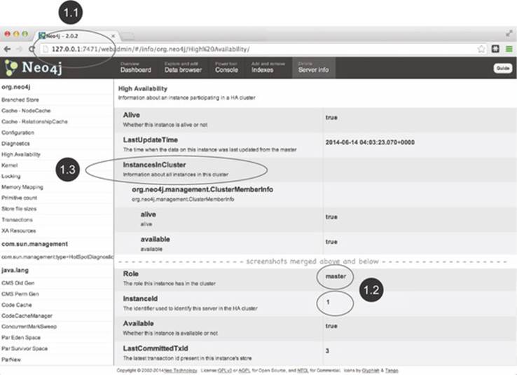
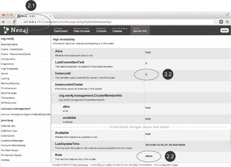
Figure 11.7. Web Admin Console view of HA setup from machine02’s perspective

In this particular startup scenario, machine01 was started first, and, as there were no other machines started in the cluster yet, machine01 assumed the role of the master, as you can see in figure 11.6 . If machine03 had started first, it would have assumed the role of the master.

The Web Admin Console provides a rich set of details about the HA cluster, including which other machines are involved in the cluster. This information can be found under the InstancesInCluster section . The first machine shown here is actually machine01, but further down the page (not shown in figure 11.6), machine02 and machine03 would also be listed as slaves, provided they had been started and successfully joined the cluster.

In figure 11.7, you can see that machine02 , having joined the cluster after machine01 was started, has taken the role of a slave .

Great! You should now have your cluster set up and running. We can now continue on to discuss some of the HA features in more detail. Feel free to experiment as we go along and try things out—this is often the best way to learn!

11.2.3. Replication—reading and writing strategies

Unlike typical master-slave replication setups that require all write requests to go through the master and read requests through slaves, Neo4j is able to handle write requests from any instance in the cluster. Likewise, Neo4j can process read requests from any instance, master or slave.

Write requests are processed quite differently depending on whether they’re received directly by the master or via a slave. Figure 11.8 shows the sequence of events that occur when a write request is sent directly to the master.

Figure 11.8. Sequence of events when a write request is sent to the master instance

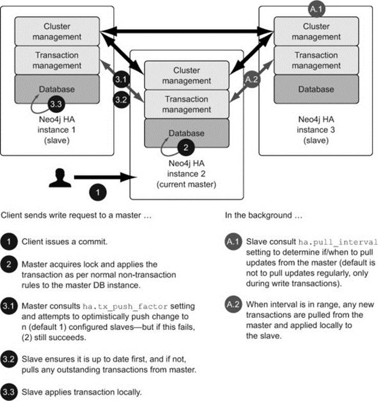
Any write requests received directly by the master will operate in much the same manner as a standard non-HA transaction does; the database acquires a lock and performs a local transaction. The only difference is that after the commit on the master has occurred, there are some configurable properties (ha.tx_push_factor and ha.tx_push_strategy) that additionally push the transaction out to n (default 1) slaves in an optimistic fashion. By optimistic, we mean that the master makes its best effort to ensure the transaction is propagated to the configured slaves, but if this propagation is unsuccessful for whatever reason, the original transaction on the master will still not fail.

Other slaves can also catch up by periodically polling for the latest updates from the master. This is done by setting the ha.pull_interval property to an appropriate value for your setup, such as 2s (every 2 seconds). This pulling and pushing mechanism is what is used to control the speed with which Neo4j becomes eventually consistent across the cluster.

Note

The use of the term optimistic here isn’t meant to be equated with the traditional database optimistic locking concept, where the whole transaction (including the one on the master) would be expected to be rolled back if a conflicted DB state is detected.

Moving on to the second scenario, if a slave receives a write request, a different sequence of events takes place, as illustrated in figure 11.9.

Figure 11.9. Sequence of events when a write request is sent to a slave instance

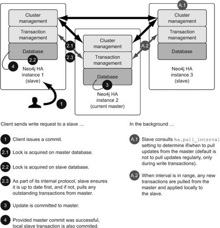
Slave-directed writes rely on the master being available in order for the update to work. This is because the slaves will synchronously need to take out a lock on both the master and slave before it can move forward. Neo4j has reliable, built-in logic to automatically detect when instances, including masters, potentially die or can’t be reached for whatever reason. In such cases, a new master is elected, and if need be, brought up to date as much as possible. If a new master is unable to be elected for whatever reason, this essentially stops all updates to the database.

Updates are always applied on the master first, and only if this is successful are they then applied to the slave. To ensure overall consistency, Neo4j requires that a slave be up to date before any writes are performed, so as part of its internal communication protocol, Neo4j will ensure that the slave has all the latest updates applied to it before performing any local writes.

Watching an update propagate through the cluster

In order to see the pulling and pushing of updates occurring within a cluster, you can play with the various Neo4j HA settings, and then, in combination with the Neo4j Web Admin Console, create nodes and relationships and watch them replicate around the cluster.

Follow these steps to try this:

1. Ensure all of your servers are up and running as described in section 11.2.2.

2. Verify on each server that there are no nodes to begin with. This can be done by going to the console tab and issuing the following Cypher query (it should return zero rows):

start n=node(*) return n;

3. On the master server, machine01 in this instance, use the Web Admin Console to create two nodes and a relationship using the following Cypher statement:

CREATE (n1)-[:LOVES]->(n2);

4. Wait until the pull interval has passed (the default value is 10 seconds—see the ha.pull_interval setting in the neo4j.properties file), and then verify that these values are now also present on the slave instances by running the query in step 2 again on each server. You should now see two nodes listed on each server.

That’s it; you’ve just seen Neo4j’s data propagation mechanism in action!

To write through the slaves—or not to write through the slaves—th- hat is the question!

Being able to send write requests to either the master or one or more slaves provides greater flexibility in deployment options, but choosing one over the other has implications that you need to consider.

· Writing through a slave will be significantly slower than writing through a dedicated master. There will naturally be higher latency involved when writing through a slave, due to the added network traffic required to sync and coordinate the data and activities of the master and slave.

· Writing through a slave can increase durability, but this can also be achieved by configuring the master to replicate changes upon commit. By writing through a slave, you’re guaranteed that there will always be at least two Neo4j instances that will always be up to date with the latest data (the slave itself, as well as the master). Alternatively, or in addition to this, durability can be increased by configuring writes on the master to be replicated out to a specified number of slaves upon commit. Although this occurs on a best-effort basis (via the ha.tx_push_factorproperty), the end result is that your data ends up on as many machines as you have configured. Distributed durability is important, as it provides a greater degree of confidence that you have the full set of data stored in multiple places, but it comes at a price.

· A load balancer of some sort will be required to ensure that writes are only, or predominantly, handled by the master. Neo4j doesn’t provide any built-in load-balancing functionality. Rather, it relies on an external mechanism of some sort to provide this capability. For clients requiring such functionality, HAProxy (www.haproxy.org) is a popular choice. The logic around when to route to the master versus a slave then needs to be built into the load-balancing mechanism, which can be a tricky proposition. How do you know if something is a read or write request? There’s generally no 100% accurate way to determine this based purely on traffic. This often results in a scenario where the application itself needs to possess some knowledge of whether its action is classified as a read or write, and then help route the request appropriately.

Whether you write through the master or a slave doesn’t have to be an all or nothing decision. It’s possible to use a hybrid approach (mostly write to the master, mostly read from the slaves) if this makes more sense for your system. Be pragmatic about making such decisions. The general recommendation provided to most clients nowadays is to try to ensure writes are predominantly sent to a master, where feasible, with data subsequently being pushed out to the slaves using the ha.tx_push_* settings. This tends to offer the best trade-off in terms of flexibility and performance.

11.2.4. Cache sharding

There will be some instances where your graph is simply too big to fit into the amount of RAM available. The advice up to now has always been to aim for this ideal situation, but what if it’s simply not possible?

In these circumstances, it’s recommended that you consider using a technique known as cache sharding. Cache sharding isn’t the same as traditional sharding.

Traditional sharding (such as the sharding employed by other data stores, like MongoDB) typically involves ensuring that different parts of the data are stored on different instances, often on different physical servers. If you have a massive customer database, you may choose to shard your database on customer groups. For example, all customers with usernames A to D are stored in one instance, E to F in another, with further divisions stored in yet others. The application would need to know which instance has the data it’s looking for and ensure that it goes to the correct one to get it. Of course, many shard-enabled databases provide automated ways of partitioning and accessing the appropriate instance, but the main point here is that not all of the data is stored on each instance or server; only a subset is.

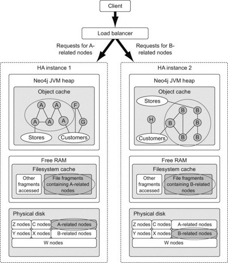
With Neo4j, each HA instance expects to have access to the full set of data. Cache sharding, unlike traditional sharding, which is a physical data partitioning technique, is more of a routing-based pattern. Using this pattern, requests for data that is typically accessed as a collective unit are always directed to the same Neo4j instance. By consistently routing such requests to the same instance, you increase the likelihood that this data will be held in memory when you access it, thereby allowing this instance to exploit the memory-accessing performance that Neo4j provides for such cases.

Let’s look again at the previous customer database example. With Neo4j, all the data (for customers A to Z) is present on each HA instance, but by using some kind of load-balancing mechanism, you can ensure that all local requests related to one group of customers (customers with “A” usernames) will always be routed to the same HA instance, “B” to another, and so on. Figure 11.10 illustrates how cache sharding might work for such a graph.

Figure 11.10. Cache sharding

Why does Neo4j not do traditional sharding?

The short answer is that this is a very, very hard problem for graph databases to solve. So hard, in fact, that this problem falls into a category of “really hard mathematical problems” that have been given their own name: “NP-hard problems” (http://en.wikipedia.org/wiki/NP-hard).

Traditional sharding typically involves splitting a full data set such that different portions are stored on different instances. Provided certain conditions hold true, this approach is a way to scale large databases while at the same time maintaining a predictable level of performance as the data grows.

The key to the preceding statement is “provided certain conditions hold true.” In most shard-enabled databases, the keys against which data is held in a shard are stable and predictable. Additionally, the access patterns generally used are such that you can look up the data you need from one shard (with a key), look up data in another, and then have the application take care of wiring it back together if required.

The sweet spot for graphs, however, and for Neo4j in particular, lies in local graph queries—starting at a given point and exploring the data and immediate connection patterns around it. This may involve traversing very different types of data—the types of data that would typically be spread across different shards. Say you had a query that said, “Given customer A, tell me which stores are within 1 km of where she lives where any of her immediate friends have purchased a product greater than £100 in the last month.” If you decided to partition data such that users and friends were stored in one shard, and retail stores in a separate area, with purchase history in yet another, a built-in graph query would end up following data spread across physical servers, resulting in unpredictable and slow data-retrieval times as the network is crossed and navigated.

You may argue that we could try to partition the data based on the pattern described, which may or may not be possible. This would, however, potentially negate other traversals that you may also want to perform—ones that start from some other node within the broader data set, not specifically customer A, and explore from there.

Until such time as we can perform such traversals across network boundaries in an acceptable and predictable manner, the best solution for such cases involving Neo4j in the interim is to make use of cache sharding. The sharding of Neo4j is still actively being looked into as a problem in its own right, but it’s not a problem that looks like it will be solved in the immediate future.

Routing strategies

As you learned in section 11.2.3, there’s no routing or load-balancing functionality built into an HA setup as far as the client is concerned; Neo4j expects clients to provide or implement their own, with tools such as HAProxy (www.haproxy.org) proving a popular choice. Regardless of the physical mechanism used, each application will need to decide on the most appropriate strategy for the routing of the data.

Some options include

· Routing requests based on some data characteristic —This is the approach used in our customer example.

· Using sticky sessions —This involves ensuring that requests from one client always go to the same server, no matter what was asked for. This may or may not be appropriate depending on the circumstances.

· Employing geography-based routing —This involves ensuring that all requests related to, or originating from, a common geographic location are always routed to the same instance.

11.2.5. HA summary

As with many of the subjects discussed in this book, we’re only able to cover a small fraction of what’s actually available, and HA is no exception. For more information on HA in general, see the “High Availability” chapter in the Neo4j Manual (chapter 23):http://docs.neo4j.org/chunked/stable/ha.html.

You’ve now learned how you can scale and ensure Neo4j can continue to operate and serve its clients, even in the event of a hardware failure. We’ll now move on to the final section in this chapter, which covers backing up and restoring the database when such disasters do actually strike.

11.3. Backups

Your social network site is whirring along nicely, generating great revenue and kudos for you, then suddenly...bam! Your administrator informs you that there was a hardware failure, and the current data is corrupted.

At this point, your heart will either sink, and you’ll say, “I really should have thought about backing the data up,” or you’ll sit back and think, “No worries, we have backups.”

Assuming you choose to be in the latter camp, this section aims to provide all the information needed to ensure that if and when such disasters do strike, you’re prepared, and it doesn’t mean the end of the world.

We’ll begin by looking at what’s involved in performing a simple offline backup, a process that does involve downtime, but one that can be performed on any edition of the Neo4j database, including the free Community edition. For the cases where you really can’t afford for the database to be offline, the online backup functionality comes into play, but this is available only in the Neo4j Enterprise edition.

11.3.1. Offline backups

At the end of the day, the physical files that comprise the Neo4j database all reside under a single directory on a filesystem, and this is what ultimately needs to be backed up. As stated in the introduction to this section, this process will work on any edition of the Neo4j database, but it will most probably only be used on the Community edition. (If you have access to the Enterprise edition, you may as well make use of the online backup functionality.)

The process itself is relatively straightforward and involves the following steps:

1. Shut down the Neo4j instance.

2. Copy the physical Neo4j database files to a backup location.

3. Restart the Neo4j instance.

Let’s look at these steps in turn.

Shut down the neo4j instance

If you’re running in a single server mode, you simply need to execute the neo4j script with a stop argument. Assuming Neo4j was installed in /opt/neo4j/bin, you could stop the server by issuing this command:

/opt/neo4j/bin/neo4j stop

If you have embedded Neo4j in your application, then unless you’ve explicitly provided a mechanism to only shut down the Neo4j database, you should stop your application with whatever mechanism you have chosen to use. This could be as simple as sending a SIGINT signal (for example, issuing Ctrl-C in a terminal window if your application has been launched in this manner), or it may be more elaborate, involving a special script or custom application functionality.

Whatever the mechanism, you should ensure that Neo4j is also shut down when this process occurs. You saw in listing 10.3 in the previous chapter what was required to ensure this occurred when running in embedded mode. To refresh your memory, here’s the snippet of code that registers a shutdown hook:

private String DB_PATH = '/var/data/neo4jdb-private';

private GraphDatabaseService graphdb =

new GraphDatabaseFactory().newEmbeddedDatabase( DB_PATH );

registerShutdownHook( graphDb );

...

private static void registerShutdownHook(

final GraphDatabaseService graphDb )

{

Runtime.getRuntime().addShutdownHook( new Thread()

{

@Override

public void run()

{

graphDb.shutdown();

}

} );

}

It’s important to ensure that Neo4j shuts down cleanly whenever your application exits; failure to do so could result in problems the next time you start up. You don’t need to worry about a clean shutdown when using Neo4j server—this will be done for you.

Copy the physical database files

Locate the directory that contains the physical Neo4j database files. For applications that run in embedded mode, this will be the path you supply in the startup code. To refresh your memory, the following snippet shows the code required to start up an embedded database where the physical files reside in the directory /var/data/neo4jdb:

private GraphDatabaseService graphdb =

new GraphDatabaseFactory().newEmbeddedDatabase("/var/data/neo4jdb" )

If you’re working with the server mode, the database files will be located at the location specified by the org.neo4j.server.database.location key in the neo4j-server.properties file. That setting will look something like the following:

org.neo4j.server.database.location=/var/data/neo4jdb

Copy the directory and all subfolders and files to a separate backup location.

Restart the database

For Neo4j server, use the appropriate Neo4j start command, and for embedded applications, restart the application as appropriate.

Note

Neo4j is able to detect unclean shutdowns and attempt a recovery, but this will result in a slower initial startup while the recovery is in process, and it sometimes may result in other issues as well. When an unclean shutdown occurs, the following warning message can generally be seen in the logs the next time the database is started up again—non clean shutdown detected. You should verify that your shut down processes, both graceful and forced, do their best to ensure Neo4j is shutdown cleanly.

11.3.2. Online backups

The online backup functionality is available only in the Enterprise edition of Neo4j, but it’s a robust and reliable way to back up your single, or clustered, Neo4j environment without requiring any downtime.

You have two options available for online backups: a full or incremental backup. In both cases, no locks are acquired on the source Neo4j instances being backed up, allowing them to continue functioning while the backup is in progress.

Full backup

A full backup essentially involves copying all of the core database files to a separate backup directory. As the database being backed up isn’t locked, there’s a very real possibility that a transaction may be running when the backup is initiated. In order to ensure that the final backup remains consistent and up to date, Neo4j will ensure that this transaction, and any others that occurred during the copy process, make it into the final backed-up files. Neo4j achieves this by making a note of any transaction IDs that were in progress when the backup began. When the copying of the core files is complete, the backup tool will then use the transaction logs (covered in section 11.1.5) to replay all transactions starting from the one just noted and including any that occurred during the copy. At the end of this process, you’ll have a fully backed up and consistent Neo4j instance.

Incremental backup

Unlike the full backup, the incremental backup doesn’t copy all of the core store files as part of its backup process. Instead, it assumes that at least one full backup has already been performed, and this backup serves as the initial starting point for identifying any changes that have subsequently occurred. The first incremental backup process will only copy over the transaction logs that have occurred since that initial full backup, thus bringing the backed-up data store to a new last-known backup point. This point is noted, and the next incremental backup will then use this as the new backup starting point, only copying over transaction logs that have occurred since that last incremental backup point up to the current point. These logs are replayed over the backup store, bringing it to the next last-known backup point. The process continues for each incremental backup requested thereafter. The incremental backup is a far more efficient process of performing a backup, as it minimizes the amount of data to be passed over the wire, as well as the time taken to actually do the backup.

The process of doing a backup

Whether or not a full or incremental backup is performed, the process for enabling and performing the backup is the same. Figure 11.11 illustrates an example backup scenario for a single server setup.

Figure 11.11. Example backup scenario for a single server setup

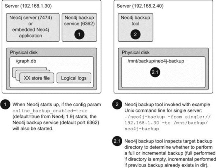
Whenever any of your Neo4j instances start up (embedded or server, single or HA), they check to see whether their online_backup_enabled configuration parameter is set to true. If it is, a separate backup service (which comes as part of the Neo4j distribution) is started as well. It defaults to port 6362 for a single server setup and 5001 for an HA setup. This service provides the access point for the Neo4j backup tool to connect to, in order to read the underlying store and transaction log files to backup.

The Neo4j backup tool is merely a Unix or Windows script (found in the bin folder of your distribution) fronting a Java application that understands how to connect to one or more Neo4j backup services. The backup tool can be run from any machine on the network, provided it has the ability to connect to the backup service. The backup command takes the following format for Unix:

./neo4j-backup –from <source-uri> -to <backup-dir>

For Windows it looks like this:

neo4j-backup –from <source-uri> -to <backup-dir>

The parameters are as follows:

· backup-dir —Directory where the backup should be stored. In order to perform a full backup, this directory needs to be empty. If the backup tool detects a previous version of a graph database in there, it will attempt an incremental backup.

· source-uri —This provides the backup tool with all the information it needs to connect to the appropriate backup service, and this needs to be specified in the following format. (Details taken from man docs found here: https://github.com/neo4j/neo4j/blob/2.0-maint/enterprise/backup/src/docs/man/neo4j-backup.1.asciidoc)

· <running-mode>://<host>[:port]{,<host>[:port]*}

·

· running-mode:

· 'single' or 'ha'. 'ha' is for instances in High

· Availability mode, 'single' is for standalone databases.

·

· host:

· In single mode, the host of a source database; in ha mode,

· the cluster address of a cluster member. Note that multiple

· hosts can be given when using High Availability mode.

·

· port:

· In single mode, the port of a source database backup service;

· in ha mode, the port of a cluster instance. If not given, the

default value 6362 will be used for single mode, 5001 for HA

How do I schedule backups?

Neo4j itself doesn’t provide any scheduling functionality. It’s expected that you’ll use an external scheduling tool (such as cron) to do this for you. Using something like cron, you can set up incremental backups to be performed every hour, or at whatever frequency suits your needs.

11.3.3. Restoring from backup

To restore a Neo4j database from a backup, simply follow these steps:

1. Shut down the specific Neo4j instance to be restored.

2. Delete the folder that contains the old or corrupted version of the Neo4j database and replace it with the backed-up version.

3. Restart the Neo4j instance.

That’s it! You’re done! It seems a bit too easy, doesn’t it? But that really is all there is to it!

11.4. Topics we couldn’t cover but that you should be aware of

Security and monitoring are two topics we couldn’t cover, but that may be worth looking into if you have specific requirements in these areas.

11.4.1. Security

Ensuring that you can run Neo4j securely in your production environment should form an important part of your configuration. Depending on how you’re making use of Neo4j, there are different aspects to consider.

There are no out-of-the-box security options provided for those making use of the embedded mode—Neo4j doesn’t provide any data-level security or encryption facilities. Most of the out-of-the-box options (as well as supplementary security configuration setups and approaches) are geared to the use of Neo4j in standalone mode (Neo4j server).

The official documentation provides relatively good coverage on the types of things to look out for, as well as basic instructions on how to begin securing these aspects of your Neo4j system. For more info, see the “Securing access to the Neo4j Server” section in the Neo4j Manual:http://docs.neo4j.org/chunked/stable/security-server.html.

11.4.2. Monitoring

Being able to monitor the health of your Neo4j system and understand when it’s getting into trouble is a good way to ensure a stable and long-running system. Most of Neo4j’s monitoring features are only available in the Enterprise edition of Neo4j, and they’re generally exposed through the Java Management Extensions (JMX) technology (http://docs.oracle.com/javase/7/docs/technotes/guides/jmx/index.html).

More information on what is available, and how to get hold of this information, can be found in the “Monitoring” chapter (chapter 26) of the Neo4j Manual: http://docs.neo4j.org/chunked/stable/operations-monitoring.html.

11.5. Summary

Congratulations! You’ve reached the end of your Neo4j journey through this book. In this final chapter, you took a tour through the high-level Neo4j architecture, periodically dipping beneath the covers, gaining some valuable insight into some of the will and whys of certain Neo4j internals, especially in the context of configuring Neo4j to operate optimally for a production environment.

Specifically, you gained insight into the factors required to calculate rough disk usage and memory requirements for your Neo4j system. You also learned about Neo4j’s two-tiered caching strategy involving the filesystem cache and object cache, and how these can be configured to suit your needs.

As this was the last chapter in the book, we recapped some of the basic concepts you encountered in the previous chapters in the book. With a solid understanding of the basic Neo4j architecture, your final task involved learning how to perform the key tasks of configuring Neo4j to run in a clustered High Availability setup, and also how to back up and recover the database.

Phew! We packed quite a bit into this last chapter, and you’ve done well to get to the end of it—congratulations!

11.6. Final thoughts

Although this chapter marks the end of this book, we hope that for you it marks the start of your onward journey with Neo4j. There’s so much more to Neo4j than we could cover; we’ve only scratched the surface here. We do hope that we’ve provided enough basic grounding and references to help you on your way as you begin to discover all that Neo4j has to offer. We’ve enjoyed writing this book and sharing our experiences with you, and we’d love to hear how you’re getting on and using Neo4j in new and interesting ways.