Neo4j in Action (2015)

Part 1. Introduction to Neo4j

What is Neo4j? What is it good for? Is it the right database for your problem domain and what kind of things can it do? In part 1 of Neo4j In Action, we’ll answer these questions and more.

Chapter 1 introduces general graph database concepts, and begins to explore some of Neo4j’s key aspects. Chapter 2 continues looking at general graph-related problems and domains, with a focus on graph data modeling techniques and approaches for various circumstances. Chapters 3 to 5are where we really start getting our hands dirty. Using an example social network of users and the movies they like, we begin exploring Neo4j starting with how to use the core API to perform the basic functionality of creating and connecting nodes, and techniques for identifying different types of nodes. Traversing graph data is also a key feature of Neo4j and chapter 4 addresses this by investigating the Neo4j Traversal API.

Chapter 5 introduces the various “indexing” strategies and options available in Neo4j, beginning by looking at the manual (legacy) option, before moving on to the built-in indexing option available from Neo4j 2.0 onward.

Chapter 1. A case for a Neo4j database

This chapter covers

· Use cases for Neo4j graph databases

· How Neo4j compares with more traditional relational databases

· Neo4j’s place in the larger NoSQL world

· Key characteristics of Neo4j

Computer science is closely related to mathematics, with a lot of its concepts originally coming from mathematical philosophy. Algorithms, cryptography, computation, automation, and even basic theories of mathematical logic and Boolean algebra are all mathematical concepts that closely couple these two disciplines. Another mathematical topic can often be found in computer science books and articles: graph theory. In computer science, graphs are used to represent specific data structures, such as organizational hierarchies, social networks, and processing flows. Typically, during the software design phase, the structures, flows, and algorithms are described with graph diagrams on a whiteboard. The object-oriented structure of the computer system is modeled as a graph as well, with inheritance, composition, and object members.

But although graphs are used extensively during the software development process, developers tend to forget about graphs when it comes to data persistence. We try to fit the data into relational tables and columns, and to normalize and renormalize its structure until it looks completely different from what it’s trying to represent.

An access control list is one example. This is a problem solved over and over again in many enterprise applications. You’d typically have tables for users, roles, and resources. Then you’d have many-to-many tables to map users to roles, and roles to resources. In the end, you’d have at least five relational tables to represent a rather simple data structure, which is actually a graph. Then you’d use an object-relational mapping (ORM) tool to map this data to your object model, which is also a graph.

Wouldn’t it be nice if you could represent the data in its natural form, making mappings more intuitive, and skipping the repeated process of “translating” the data to and from a storage engine? Thanks to graph databases, you can. Graph databases use the graph model to store data as a graph, with a structure consisting of vertices and edges, the two entities used to model any graph.

In addition, you can use all the algorithms from the long history of graph theory to solve graph problems more efficiently and in less time than using relational database queries.

Once you’ve read this book, you’ll be familiar with Neo4j, one of the most prominent graph databases available. You’ll learn how a Neo4j graph database helps you model and solve graph problems in a better-performing and more elegant way, even when working with large data sets.

1.1. Why Neo4j?

Why would you use a graph database, or more specifically Neo4j, as your database of choice? As mentioned earlier, it’s often quite natural for people to logically try to model, or describe, their particular problem domain using graph-like structures and concepts, even though they may not use a graph database as their ultimate data store. Choosing the right data store (or data stores—plural, in today’s polyglot persistence world) to house your data can make your application soar like an eagle; it can come crashing to the ground just as easily if the wrong choice is made.

A good way to answer this question, then, is to take a problem that naturally fits very well into the graph-based world and compare how a solution using Neo4j fares against one using a different data store. For comparison purposes, we’ll use a traditional relational database, as this is generally the lowest common denominator for most people when it comes to understanding data storage options. More importantly, it’s what most people have turned to—and sometimes still turn to—to model such problems.

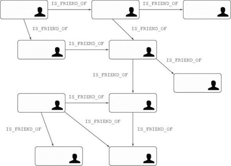
The example we’re going to explore is a social network—a set of users who can be friends with each other. Figure 1.1 illustrates the social network, where users connected with arrows are friends.

Figure 1.1. Users and their friends represented as a graph data structure

Note

To be semantically correct, the friendship relationship should be bidirectional. In Neo4j, bidirectionality is modeled using two relationships, with one direction each. (In Neo4j, each relationship must have a well-defined direction, but more on that later.) So you should see two separate friendship relationships for each pair of friends, one in each direction. For simplicity we have modeled friendships as single, direct relationships. In chapters 2 and 3 you’ll learn why this data model is actually more efficient in Neo4j.

Let’s look at the relational model that would store data about users and their friends.

1.2. Graph data in a relational database

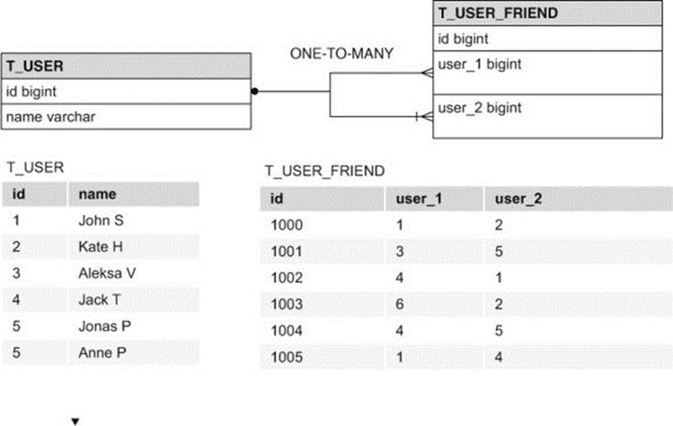
In a relational database, you’d typically have two relational tables for storing social network data: one for user information, and another for the relationships between users (see figure 1.2).

Figure 1.2. SQL diagram of tables representing user and friend data

The following listing shows the SQL script for creating tables using a MySQL database.

Listing 1.1. SQL script defining tables for social network data

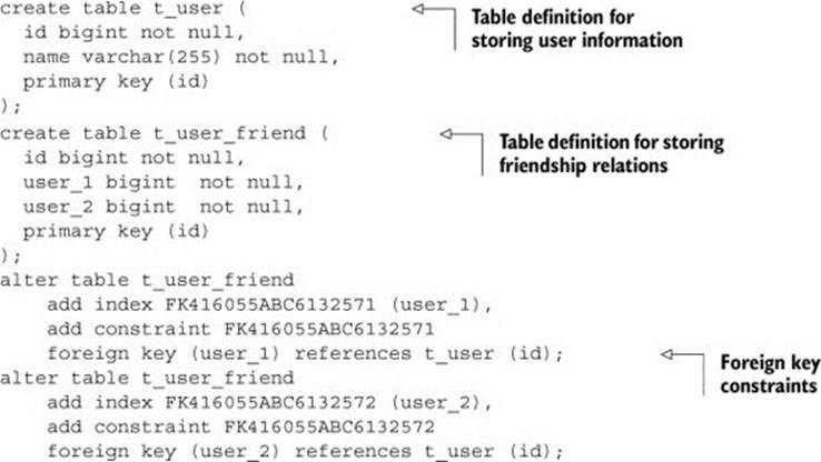
Table t_user contains columns with user information, while table t_user_friend simply has two columns referencing table t_user using a foreign key relation. The primary key and foreign key columns have indexes for quicker lookup operations, a strategy typically employed when modeling relational databases.

1.2.1. Querying graph data using MySQL

How would you go about querying relational data? Getting the count for direct friends of a particular user is quite straightforward. A basic select query such as the following would do the trick:

select count(distinct uf.*) from t_user_friend uf where uf.user_1 = ?

Note

We’re counting the friends in all examples, so we don’t overload the CPU or memory by loading the actual data.

How about finding all friends of a user’s friends? This time you’d typically join the t_user_friend table with itself before querying:

select count(distinct uf2.*) from t_user_friend uf1

inner join t_user_friend uf2 on uf1.user_1 = uf2.user_2

where uf1.user_1 = ?

Popular social networks usually have a feature where they suggest people from your friendship network as potential friends or contacts, up to a certain degree of separation, or depth. If you wanted to do something similar to find friends of friends of friends of a user, you’d need another joinoperation:

select count(distinct uf3.*) from t_user_friend uf1

inner join t_user_friend uf2 on uf1.user_1 = uf2.user_2

inner join t_user_friend uf3 on uf2.user_1 = uf3.user_2

where uf1.user_1 = ?

Similarly, to iterate through a fourth level of friendship, you’d need four joins. To get all connections for the famous six degrees of separation problem, six joins would be required.

There’s nothing unusual about this approach, but there’s one potential problem: although you’re only interested in friends of friends of a single user, you have to perform a join of all data in the t_user_friend table, and then discard all rows that you’re not interested in. On a small data set, this wouldn’t be a big concern, but if your social network grows large, you could start running into serious performance problems. As you’ll see, this can put a huge strain on your relational database engine.

To illustrate the performance of such queries, we ran the friends-of-friends query a few times against a small data set of 1,000 users, but increased the depth of the search with each invocation and recorded the results each time. On a small data set of 1,000 users, where each user has on average 50 friends, table t_user contains 1,000 records, whereas table t_user_friend contains 1,000 × 50 = 50,000 records.

At each depth, we ran the query 10 times—this was simply to warm up any caches that could help with performance. The fastest execution time for each depth was recorded. No additional database performance tuning was performed, apart from column indexes defined in the SQL script from listing 1.1. Table 1.1 shows the results of the experiment.

Table 1.1. Execution times for multiple join queries using a MySQL database engine on a data set of 1,000 users

Note

All experiments were executed on an Intel i7–powered commodity laptop with 8 GB of RAM, the same computer that was used to write this book.

Note

With depths 3, 4, and 5, a count of 999 is returned. Due to the small data set, any user in the database is connected to all others.

As you can see, MySQL handles queries to depths 2 and 3 quite well. That’s not unexpected—join operations are common in the relational world, so most database engines are designed and tuned with this in mind. The use of database indexes on the relevant columns also helped the relational database to maximize its performance of these join queries.

At depths 4 and 5, however, you see a significant degradation of performance: a query involving 4 joins takes over 10 seconds to execute, while at depth 5, execution takes way too long—over a minute and a half, although the count result doesn’t change. This illustrates the limitation of MySQL when modeling graph data: deep graphs require multiple joins, which relational databases typically don’t handle too well.

Inefficiency of SQL joins

To find all a user’s friends at depth 5, a relational database engine needs to generate the Cartesian product of the t_user_friend table five times. With 50,000 records in the table, the resulting set will have 50,000⁵ rows (102.4 × 10²¹), which takes quite a lot of time and computing power to calculate. Then you discard more than 99% to return the just under 1,000 records that you’re interested in!

As you can see, relational databases are not so great for modeling many-to-many relationships, especially in large data sets. Neo4j, on the other hand, excels at many-to-many relationships, so let’s take a look at how it performs with the same data set. Instead of tables, columns, and foreign keys, you’re going to model users as nodes, and friendships as relationships between nodes.

1.3. Graph data in Neo4j

Neo4j stores data as vertices and edges, or, in Neo4j terminology, nodes and relationships. Users will be represented as nodes, and friendships will be represented as relationships between user nodes. If you take another look at the social network in figure 1.1, you’ll see that it represents nothing more than a graph, with users as nodes and friendship arrows as relationships.

There’s one key difference between relational and Neo4j databases, which you’ll come across right away: data querying. There are no tables and columns in Neo4j, nor are there any SQL-based select and join commands. So how do you query a graph database?

The answer is not “write a distributed MapReduce function.” Neo4j, like all graph databases, takes a powerful mathematical concept from graph theory and uses it as a powerful and efficient engine for querying data. This concept is graph traversal, and it’s one of the main tools that makes Neo4j so powerful for dealing with large-scale graph data.

1.3.1. Traversing the graph

The traversal is the operation of visiting a set of nodes in the graph by moving between nodes connected with relationships. It’s a fundamental operation for data retrieval in a graph, and as such, it’s unique to the graph model. The key concept of traversals is that they’re localized—querying the data using a traversal only takes into account the data that’s required, without needing to perform expensive grouping operations on the entire data set, like you do with join operations on relational data.

Neo4j provides a rich Traversal API, which you can employ to navigate through the graph. In addition, you can use the REST API or Neo4j query languages to traverse your data. We’ll dedicate much of this book to teaching you the principles of and best practices for traversing data with Neo4j.

To get all the friends of a user’s friends, run the code in the following listing.

Listing 1.2. Neo4j Traversal API code for finding all friends at depth 2

TraversalDescription traversalDescription =

Traversal.description()

.relationships("IS_FRIEND_OF", Direction.OUTGOING)

.evaluator(Evaluators.atDepth(2))

.uniqueness(Uniqueness.NODE_GLOBAL);

Iterable<Node> nodes = traversalDescription.traverse(nodeById).nodes();

Don’t worry if you don’t understand the syntax of the code snippet in listing 1.2—everything will be explained slowly and thoroughly in the next few chapters. Figure 1.3 illustrates the traversal of the social network graph, based on the preceding traversal description.

Figure 1.3. Traversing the social network graph data

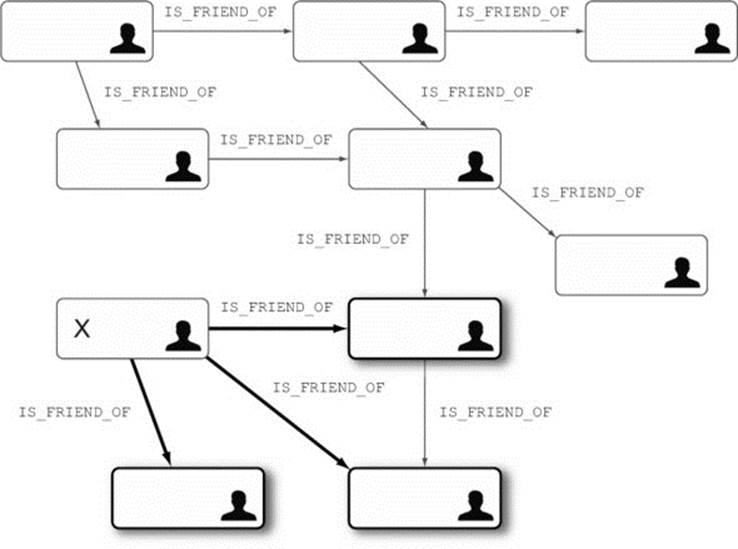
Before the traversal starts, you select the node from which the traversal will start (node X in figure 1.3). Then you follow all the friendship relationships (arrows) and collect the visited nodes as results. The traversal continues its journey from one node to another via the relationships that connect them. The direction of relationships does not affect the traversal—you can go up and down the arrows with the same efficiency. When the rules stop applying, the traversal stops. For example, the rule can be to visit only nodes that are at depth 1 from the starting node, in which case once all nodes at depth 1 are visited, the traversal stops. (The darker arrows in figure 1.3 show the relationships that are followed for this example.)

Table 1.2 shows the performance metrics for running a traversal against a graph containing the same data that was in the previous MySQL database (where the traversal is functionally the same as the queries executed previously on the database, finding friends of friends up the defined depth). Again, this is for a data set of 1,000 users with an average of 50 friends per user.

Table 1.2. The execution times for graph traversal using Neo4j on a data set of 1,000 users

Note

Similar to the MySQL setup, no additional performance tuning was done on the Neo4j instance. Neo4j was running in embedded mode, with the default configuration and 2,048 MB of JVM heap memory.

The first thing to notice is that the Neo4j performance is significantly better for all queries, except the simplest one. Only when looking for friends of friends (at depth 2) is the MySQL performance comparable to the performance of a Neo4j traversal. The traversal of friends at depth 3 is four times faster than the MySQL counterpart. When performing a traversal at depth 4, the results are five orders of magnitude better. The depth 5 results are 10 million times faster for the Neo4j traversal compared to the MySQL query!

Another conclusion that can be made from the results in table 1.2 is that the performance of the query degrades only slightly with the depth of the traversal when the count of nodes returned remains the same. The MySQL query performance degrades with the depth of the query because of the Cartesian product operations that are executed before most of the results are discarded. Neo4j keeps track of the nodes visited, so it can skip nodes it’s visited before and therefore significantly improve performance.

To find all friends at depth 5, MySQL will perform a Cartesian product on the t_user_friend table five times, resulting in 50,000⁵ records, out of which all but 1,000 are discarded. Neo4j will simply visit nodes in the database, and when there are no more nodes to visit, it will stop the traversal. That is why Neo4j can maintain constant performance as long as the number of nodes returned remains the same, whereas there’s a significant degradation in performance when using MySQL queries.

Note

Graph traversals perform significantly better than the equivalent MySQL queries (thousands of times better with traversal depths of 4 and 5). At the same time, the traversal performance does not decrease dramatically with the depth—the traversal at depth 5 is only 0.03 seconds slower than the traversal at depth 2. The performance of the most complex MySQL queries is more than 10,000 times slower than the simple ones.

But how does this graphing approach scale? To get the answer, let’s repeat the experiment with a data set of 1 million users.

1.4. SQL joins versus graph traversal on a large scale

For this experiment, we used exactly the same data structures as before; the only difference was the amount of data.

In MySQL we had 1,000,000 records in the t_user table, and approximately 1,000,000 × 50 = 50,000,000 records in the t_user_friend table. We ran the same four queries against this data set (friends at depths 2, 3, 4, and 5). Table 1.3 shows the collected results for the performance of SQL queries in this case.

Table 1.3. The execution times for multiple join queries using a MySQL database engine on a data set of 1 million users

Comparing these results to the MySQL results for a data set of 1,000 users, you can see that the performance of the depth 2 query has stayed the same, which can be explained by the design of the MySQL engine handling table joins efficiently using indexes. Queries at depths 3 and 4 (which use 3 and 4 join operations, respectively) demonstrate much worse results, by at least two orders of magnitude. The SQL query for all friends at depth 5 did not finish in the hour we ran the script.

Note

To store the large amount of data required for these examples, a significant amount of disk space is required. To generate the sample data and run examples against it, you’ll need in excess of 10 GB of disk space available.

These results clearly show that the MySQL relational database is optimized for single join queries, even on large data sets. The performance of multiple join queries on large data sets degrades significantly, to the point that some queries are not even executable (for example, friends at depth 5 for a data set of 1 million users).

Why are relational database queries so slow?

The results in table 1.3 are somewhat expected, given the way join operations work. As we discussed earlier, each join creates a Cartesian product of all potential combinations of rows, then filters out those that don’t match the where clause. With 1 million users, the Cartesian product of 5 joins (equivalent to a query at depth 5) contains a huge number of rows—billions. Way too many zeros to be readable. Filtering out all the records that don’t match the query is too expensive, such that the SQL query at depth 5 never finishes in a reasonable time.

We repeated the same experiment with Neo4j traversals. We had 1 million nodes representing users, and approximately 50 million relationships stored in Neo4j. We ran the same four traversals as in the previous example, and we got the performance results in table 1.4.

Table 1.4. The execution times for graph traversal using Neo4j on a data set of 1 million users

As you can see, the increase in data by a thousand times didn’t significantly affect Neo4j’s performance. The traversal does get slower as you increase the depth, but the main reason for that is the increased number of results that are returned. The performance slows linearly with the increase of the result size, and it’s predictable even with a larger data set and depth level. In addition, this is at least a hundred times better than the corresponding MySQL performance.

The main reason for Neo4j’s predictability is the localized nature of the graph traversal; irrespective of how many nodes and relationships are in the graph, the traversal will only visit ones that are connected to the starting node, according to the traversal rules. Remember, relational joinoperations compute the Cartesian product before discarding irrelevant results, affecting performance exponentially with the growth of the data set. Neo4j, however, only visits nodes that are relevant to the traversal, so it’s able to maintain predictable performance regardless of the total data set size. The more nodes the traversal has to visit, the slower the traversal, as you’ve seen while increasing the traversal depth. But this increase is linear and is still independent of the total graph size.

What is the secret of Neo4j’s speed?

No, Neo4j developers haven’t invented a superfast algorithm for the military. Nor is Neo4j’s speed a product of the fantastic speed of the technologies it relies on (it’s implemented in Java after all!).

The secret is in the data structure—the localized nature of graphs makes it very fast for this type of traversal. Imagine yourself cheering on your team at a small local football stadium. If someone asks you how many people are sitting 15 feet around you, you’ll get up and count them—you’ll count people around you as fast as you can count. Now imagine you’re attending the game at the national stadium, with a lot more spectators, and you want to answer the same question—how many people are there within 15 feet of you. Given that the density of people in both stadiums is the same, you’ll have approximately the same number of people to count, taking a very similar time. We can say that regardless of how many people can fit into the stadium, you’ll be able to count the people around you at a predictable speed; you’re only interested in the people sitting 15 feet around you, so you won’t be worried about packed seats on the other end of the stadium, for example.

This is exactly how the Neo4j engine works in the example—it visits nodes connected to the starting node, at a predictable speed. Even when the number of nodes in the whole graph increases (given similar node density), the performance can remain predictably fast.

If you apply the same football analogy to the relational database queries, you’d count all the people in the stadium and then remove those not around you, which is not the most efficient strategy given the interconnectivity of the data.

These experiments demonstrate that the Neo4j graph database is significantly faster in querying graph data than using a relational database. In addition, a single Neo4j instance can handle data sets of three orders of magnitude without performance penalties. The independence of traversal performance on graph size is one of the key aspects that make Neo4j an ideal candidate for solving graph problems, even when data sets are very large.

In the next section we’ll try to answer the question of what graph data actually is, and how Neo4j can help you model your data models as natural graph structures.

1.5. Graphs around you

Graphs are considered the most ubiquitous natural structures. The first scientific paper on graph theory is considered to be a solution of the historical seven bridges of Königsberg problem, written by Swiss mathematician Leohnard Euler in 1774. The seven bridges problem started what is now known as graph theory, and its model and algorithms are now applied across wide scientific and engineering disciplines.

There are a lot of examples of graph usage in modern science. For example, graphs are used to describe the relative positions of the atoms and molecules in chemical compounds. The laws of atomic connections in physics are also described using graphs. In biology, the evolution tree is actually a special form of graph. In linguistics, graphs are used to model semantic rules and syntax trees. Network analysis is based on graph theory as well, with applications in traffic modeling, telecommunications, and topology.

In computer science, a lot of problems are modeled as graphs: social networks, access control lists, network topologies, taxonomy hierarchies, recommendation engines, and so on. Traditionally, all of these problems would use graph object models (implemented by the development team), and store the data in normalized form in a set of tables with foreign key associations.

In the previous section you saw how a social network can be stored in the relational model using two tables and a foreign key constraint. Using a Neo4j graph database, you can preserve the natural graph structure of the data, without compromising performance or storage space, therefore improving the query performance significantly.

When using a Neo4j graph database to solve graph problems, the amount of work for the developer is reduced, as the graph structures are already available via the database APIs. The data is stored in its natural format—as graph nodes and relationships—so the effects of an object-relational mismatch are minimized. And the graph query operations are executed in an efficient and performant way by using the Neo4j Traversal API. Throughout this book we’ll demonstrate the power of Neo4j by solving problems such as access control lists and social networks with recommendation engines.

If you’re not familiar with graph theory, don’t worry; we’ll introduce some of the graph theory concepts and algorithms, as well as their applicability to graph storage engines such as Neo4j, when they become relevant in later chapters.

In the next section we’ll discuss the reasons why graph databases (and other NoSQL technologies) started to gain popularity in the computer industry. We’ll also discuss categories of NoSQL systems with a focus on their differences and applicability.

1.6. Neo4j in NoSQL space

Since the beginning of computer software, the data that applications have had to deal with has grown enormously in complexity. The complexity of the data includes not only its size, but also its interconnectedness, its ever-changing structure, and concurrent access to the data.

With all these aspects of changing data, it has been recognized that relational databases, which have for a long time been the de facto standard for data storage, are not the best fit for all problems that increasingly complex data requires. As a result, a number of new storage technologies has been created, with a common goal of solving the problems relational databases are not good at. All these new storage technologies fall under the umbrella term NoSQL.

Note

Although the NoSQL name stuck, it doesn’t accurately reflect the nature of the movement, giving the (wrong) impression that it’s against SQL as a concept. A better name would probably be nonrelational databases, as the relational/nonrelational paradigm was the subject of discussion, whereas SQL is just a language used with relational technologies.

The NoSQL movement was born as an acknowledgment that new technologies were required to cope with the data changes. Neo4j, and graph databases in general, are part of the NoSQL movement, together with a lot of other, more or less related storage technologies.

With the rapid developments in the NoSQL space, its growing popularity, and a lot of different solutions and technologies to choose from, anyone new coming into the NoSQL world faces many choices when selecting the right technology. That’s why in this section we’ll try to clarify the categorization of NoSQL technologies and focus on the applicability of each category. In addition, we’ll explain the place of graph databases and Neo4j within NoSQL.

1.6.1. Key-value stores

Key-value stores represent the simplest, yet very powerful, approach to handling high-volume concurrent access to data. Caching is a typical key-value technology. Key-value stores allow data to be stored using very simple structures, often in memory, for very fast access even in highly concurrent environments.

The data is stored in a huge hash table and is accessible by its key. The data takes the form of key-value pairs, and the operations are mostly limited to simple put (write) and get (read) operations. The values support only simple data structures like text or binary content, although some more recent key-value stores support a limited set of complex data types (for example, Redis supports lists and maps as values).

Key-value stores are the simplest NoSQL technologies. All other NoSQL categories build on the simplicity, performance, and scalability of key-value stores to better fit some specific use cases.

1.6.2. Column-family stores

The distributed key-value model scaled very well but there was a need to use some sort of data structure within that model. This is how the column-family store category came on the NoSQL scene.

The idea was to group similar values (or columns) together by keeping them in the same column family (for example, user data or information about books). Using this approach, what was a single value in a key-value store evolved to a set of related values. (You can observe data in a column-family store as a map of maps, or a key-value store where each value is another map.) The column families are stored in a single file, enabling better read and write performance on related data. The main goal of this approach was high performance and high availability when working with big data, so it’s no surprise that the leading technologies in this space are Google’s BigTable and Cassandra, originally developed by Facebook.

1.6.3. Document-oriented databases

A lot of real problems (such as content management systems, user registration data, and CRM data) require a data structure that looks like a document. Document-oriented databases provide just such a place to store simple, yet efficient and schemaless, document data. The data structure used in this document model enables you to add self-contained documents and associative relationships to the document data.

You can think of document-oriented databases as key-value stores where the value is a document. This makes it easier to model the data for common software problems, but it comes at the expense of slightly lower performance and scalability compared to key-value and column-family stores. The convenience of the object model built into the storage system is usually a good trade-off for all but massively concurrent use cases (most of us are not trying to build another Google or Facebook, after all).

1.6.4. Graph databases

Graph databases were designed with the view that developers often build graph-like structures in their applications but still store the data in an unnatural way, either in tables and columns of relational databases, or even in other NoSQL storage systems. As we mentioned before, problems like ACL lists, social networks, or indeed any kind of networks are natural graph problems. The graph data model is at the core of graph databases—you’re finally able to store an object model that represents graph data as a persisted graph!

This data model can naturally represent a lot of complex software requirements and the efficiency and performance of graph traversal querying are the main strengths of graph databases.

1.6.5. NoSQL categories compared

Table 1.5 illustrates the use cases and representative technologies for each of the NoSQL categories.

Table 1.5. An overview of NoSQL categories

So far in this chapter, you’ve seen examples of the efficient use of Neo4j to solve graph-related problems, seen how common real-world problems can be naturally modeled as graphs, and learned where graph databases and Neo4j in particular sit within the wider NoSQL space. But there’s one key aspect of Neo4j that none of the other NoSQL stores have—one that’s very important when it comes to the adoption of new storage technologies in the enterprise world: transactional behavior.

1.7. Neo4j: the ACID-compliant database

Transaction management has been a prominent talking point in discussions of NoSQL technologies since they started to gain popularity. Trading off transactional attributes for increased performance and scalability has been a common approach in nonrelational technologies that targeted big data. Some (such as BigTable, Cassandra, and CouchDB) opted to trade off consistency, allowing clients to read stale data in some cases in a distributed system (eventual consistency). In key-value stores that concentrated on read performance (such as Memcached), durability of the data wasn’t of too much interest. Similarly, atomicity on a single-operation level, without the possibility to wrap multiple database operations within a single transaction, is typical for document-oriented databases.

While each of the approaches mentioned here are valid in specific use cases (such as caching, high data-read volumes, high load, and concurrency), the lack of ACID-based transaction handling is usually the first hurdle when it comes to introducing nonrelational databases to any enterprise or corporate environment. Although they were devised a long time ago for relational databases, transaction attributes still play an important and fundamental part in many practical use cases. Neo4j has therefore taken a different approach.

Neo4j’s goal is to be a graph database, with the emphasis on database. This means that you’ll get full ACID support from the Neo4j database:

· Atomicity (A) —You can wrap multiple database operations within a single transaction and make sure they’re all executed atomically; if one of the operations fails, the entire transaction will be rolled back.

· Consistency (C) —When you write data to the Neo4j database, you can be sure that every client accessing the database afterward will read the latest updated data.

· Isolation (I) —You can be sure that operations within a single transaction will be isolated one from another, so that writes in one transaction won’t affect reads in another transaction.

· Durability (D) —You can be certain that the data you write to Neo4j will be written to disk and available after database restart or a server crash.

Note

It’s very important to note that Neo4j is a transactional database. Everything you know about transactions from the relational world applies to Neo4j as well. Transaction support is one the key differentiators between Neo4j and the other NoSQL databases we mentioned earlier, which don’t support all ACID properties.

The ACID transactional support provides a seamless transition to Neo4j for anyone used to the guarantees provided by relational databases, and it offers safety and convenience in working with graph data. Transactional support is one of the strong points of Neo4j, which differentiates it from the majority of NoSQL solutions and makes it a good option not only for NoSQL enthusiasts, but in enterprise environments as well.

1.8. Summary

In this chapter you learned how much more efficient and performant Neo4j can be compared to relational databases for solving specific problems, such as the social network in the example. We illustrated the performance and scalability benefits of graph databases, as represented by Neo4j, showing the clear advantage Neo4j has over a relational database when dealing with graph-related problems.

You also learned about some of the key characteristics of Neo4j, as well as its place within the larger NoSQL movement of related data-storage technologies.

Using graph databases to store the data affects the way you should think about data. This is where data modeling becomes very important. There are no tables and columns any more, like in relational databases, or keys and values, like in other NoSQL technologies. You have to switch your mind to think of graph representations of your data. In the next chapter we’ll give you some guidance and explain the best practices for modeling your graph data.