JavaScript and jQuery for Data Analysis and Visualization (2015)
PART III Visualizing Data Programmatically
Chapter 11 Introducing D3
What's in This Chapter
· Getting started with D3
· Creating, manipulating, and destroying data-driven elements
· Working with D3 transitions
· Dealing with visually complex, nested data structures.
· Exploring D3's toolkit of functions for simplifying common tasks.
· Building a file system visualization using a built-in D3 layout.
CODE DOWNLOAD The wrox.com code downloads for this chapter are found at www.wrox.com/go/javascriptandjqueryanalysis on the Download Code tab. The code is in the chapter 11 download and individually named according to the names throughout the chapter.
D3 is a JavaScript library for general purpose visualization. D3 possesses a powerful selection model for declaratively describing how data should be mapped to the visual elements. It comes bundled with a vast variety of helper functions that can be leveraged when building visualizations and is easily extensible to support custom functionality.
Unlike some other visualization libraries, D3 does not offer any prepackaged “standard” visualizations (bar chart, pie chart, and so on), although you can create your own. If you are only interested in standard quick visualizations then you should check out some of the libraries written on top of D3, such as NVD3 (http://nvd3.org/) and C3.js (http://c3js.org/).
On the surface, D3 appears to be similar to jQuery with regard to selecting and manipulating existing elements on the page. D3 adds a mechanism for adding or removing elements to match a dataset, which makes it particularly apt for data visualization.
The true power (and joy) of using D3 comes from the ability to take a data set and turn it into a fully customized interactive visualization by assigning visual elements to data items and leveraging the vast suite of built-in helper functions.
Imagine looking at a dataset of all U.S. hospitals that list the name, city, state, owner, and location for each facility. See Figure 11.1 for an example of what some rows for the dataset would look like.
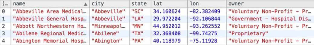
Figure 11.1 This table shows the first five rows of the hospital data set.
You could be interested in the distribution of hospitals by state visualized as a bar chart, as shown in Figure 11.2. Alternatively you could grab a geo JSON representation of the United States from the census bureau, pick one of D3's geo-projection functions, and plot every hospital on a map. You could then use a Voronoi layout (discussed in Chapter 16) to visualize each hospital's catchment area as shown in Figure 11.3. These examples, with fully annotated source code, can be found in the us-hospitals directory in the Chapter 11 code examples on the companion website.
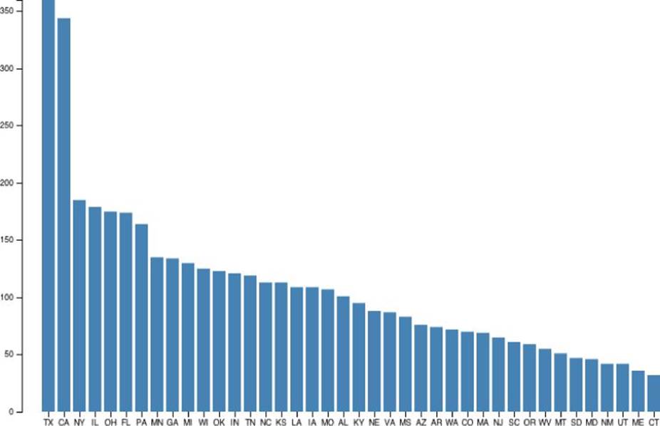
Figure 11.2 This bar chart shows the distribution of hospitals by state.
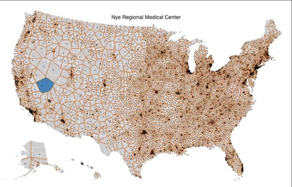
Figure 11.3 This geo-visualization shows U.S. hospitals with their areas of influence.
This chapter dives into D3's core concepts: element selections, data joining, and transitions. The D3 community has experienced meteoric growth, and there is no shortage of examples, tutorials, and how-tos online. The aim here is to give you a good framework for understanding any D3 visualization that you might encounter in the wild and give you the ability to remix them or create your own.
Getting Started
The following is the basic structure of the HTML that would house a D3 visualization. (You can find this file in the blank/index.html directory for Chapter 11 on the companion website.)
<!DOCTYPE html>
<html>
<head>
<meta charset='utf-8'>
<script src="../d3/d3.js" charset="utf-8"></script>
<link rel="stylesheet" href="../common.css">
<link rel="stylesheet" href="style.css">
<title>My visualization</title>
</head>
<body>
<script src="script.js"></script>
</body>
</html>
The examples in this chapter use a local copy of D3 so that they may function offline, but a hosted version is also available. To get the latest release in your project, copy this snippet into the <head> part of the document:
<script src="http://d3js.org/d3.v3.min.js" charset="utf-8"></script>
Alternatively, you can play around with D3 by using an online web development playground such as http://jsfiddle.net/. You simply need to select D3 in the sidebar as a library to load and start playing.
DOM and SVG
D3 acts on elements within the page. It can manipulate any element that implements the Document Object Model (DOM) interface. This includes HTML elements (like <div> and <table>) and SVG elements.
SVG stands for Scalable Vector Graphics, and is a standard that can create visuals out of vector primitives such as lines and circles. SVG is a good choice for visualization because it is based on a DOM, allowing its elements to have events and to be manipulated with D3 selections. SVG can also be scaled to any size without degradation of quality. Figure 11.4 shows a very simple SVG element containing four rectangles.
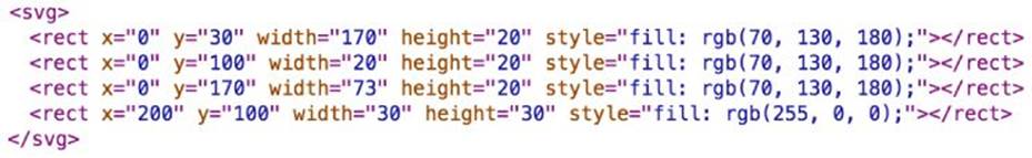
Figure 11.4 Shown here is a representation of an SVG element as presented in the Google Chrome inspector panel.
Because SVG maintains a scene graph of the visual elements displayed, there is some overhead ascribed per element. A visualization that involves hundreds of thousands of elements might be more appropriately implemented using the HTML5 Canvas component. Canvas acts as a simple bitmap container to put you in charge of interpreting the locations of mouse events and coordinate systems.
In this chapter the focus is on applying D3 to create SVG graphics, as it is the most common medium for the task.
Unlike some other visualization tools (such as http://raphaeljs.com/) D3 expects you to know and understand the underlying technology into which your visualization is going to be rendered (be it SVG or HTML). As such, it is recommended that you have a reference book at hand to be able to look up the correct usage of different elements. One good SVG reference is SVG Essentials by J. David Eisenberg and Amelia Bellamy-Royds (O'Reilly Media, 2014).
It should also be noted that modern browsers come with powerful debugging tools that enable you to see the structure of the document in them. This is a great way to familiarize yourself with SVG (and HTML) as you can always examine the structure of any SVG-based visualization you will find online or in this chapter. Right-click any element and select Inspect Element to see the internal structure of the page. Figure 11.5 shows the Inspect Element menu for the visualization in Figure 11.3.
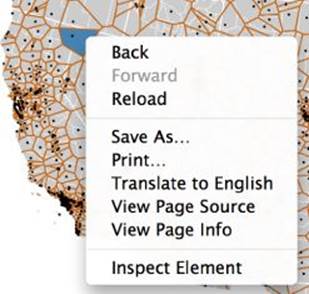
Figure 11.5 The single most useful tool for web development is the inspector console.
.select
The principal data structure in D3 is the selection. Selections represent sets of elements and provide operators that can be applied to the selected elements. These operators wrap the element's DOM interface, setting attributes (attr), inline styles (style), and text content (text). Operator values are specified either as constants or functions; the latter are evaluated for each element.
The selection.select(selector) function uses a CSS selector string to find the first element within the selection that matches the selector. It then constructs a new selection containing the found element. Calling d3.select(selector) runs over the entire document.
Start with a document containing an SVG with a single rectangle. In reality, you would rarely start from this state, but bear with it for now:
<svg>
<rect x="150" y="100" width="60" height="123"></rect>
</svg>
Now perform a simple selection:
var svg = d3.select("svg")
svg.select("rect")
.attr("width", 100)
.attr("height", 100)
.style("fill", "steelblue")
.style("stroke-width", 3)
.style("stroke", "#FFC000")
The result is a square, as shown in Figure 11.6. (You can find this file in the select/script.js directory in the Chapter 11 code examples on the companion website.)

Figure 11.6 This rectangle had its attributes modified to become a square.
The preceding code selects the <svg> element in the page and stores it in a variable called svg. It then selects the <rect> element within svg and modifies its attributes and styles. For brevity, the attr and style operations are chained together because each returns the selection.
.selectAll
Although .select is an invaluable tool, your visualization will rarely be composed of a single element. .selectAll works like .select but selects all elements that match. The elements in the selection created by .selectAll can be manipulated concurrently using the attrand style operators.
These operators can receive two types of input:
· They can receive a value (.attr("x", 0)) and apply that value to all the elements.
· They can receive a function (.attr("y", function(d, i) { return i * 70 + 30 })) that will “run” once per element to compute an element-specific value for the attribute. The first parameter to this function, commonly labeled d, represents the data associated to the element (which is examined in the next section), and the second parameter, commonly labeled i, represents the index of the element in the DOM.
Start with a document containing an SVG with several rectangles:
<svg>
<rect x="150" y="100" width="60" height="123"></rect>
<rect x="80" y="10" width="20" height="50"></rect>
<rect x="30" y="130" width="60" height="23"></rect>
</svg>
Now perform a simple selectAll (refer to the /selectAll/script.js directory in the Chapter 11 code on the companion website):
var svg = d3.select("svg")
svg.selectAll("rect")
.attr("x", 0)
.attr("y", function(d, i) { return i * 70 + 30 })
.attr("width", function(d, i) { return i * 50 + 100 })
.attr("height", 20)
.style("fill", "steelblue")
As you can see, in Figure 11.7, the three rectangles have been repositioned to resemble a bar chart (albeit a bar chart that is not representing any kind of data).

Figure 11.7 The three rectangles have been rearranged.
The <svg> is selected like before. After all the <rect>s in the SVG are selected, you apply a series of attributes and styles to all of them.
Notice these lines of code:
.attr("y", function(d, i) { return i * 70 + 30 })
.attr("width", function(d, i) { return i * 50 + 100 })
Instead of a value, you provide the attr operator with a function that will be evaluated for every element in the selection. By using the index, you specified different y and width attributes for every element making the bars appear similar to a bar chart. The actual formulas used to size the bars (i * 70 + 30) in this example are arbitrary; soon you find out how to connect this to real data.
D3 always interprets the argument provided to the operands as a function so writing this:
.style("fill", "steelblue")
is simply shorthand for this:
.style("fill", function() {
return "steelblue"
})
.data() (Also Known As Data Joining)
Now that you have seen the basics of how to select elements and assign their attributes declaratively, it's time to dive into the heart of D3: joining data to visual elements.
The selection.data operator binds an array of data to the elements of the selection. The first argument is the data to be bound— specified as an array of arbitrary values (such as numbers, strings, or objects). By default the members of the data array are joined to the elements by their index. This behavior can be modified by supplying a key function, which is covered later in the “Key Functions” section.
When data is joined with a selection of elements, three new selections are created:
· Elements that already represent data but might need to be updated (update)
· Data that has no element representing it yet (enter)
· Elements that no longer have data to represent (exit)
The D3 terms “enter” and “exit” originate from the metaphor of directions in theatrical scripts. Metaphorically the datum is an actor, and the elements are costumes. When an actor enters the stage he needs to put on a costume, which is what the audience sees. Similarly, when an actor exits the stage he disappears as far as the audience is concerned.
Let's examine these new selections one-by-one.
Update
The new selection returned by the .data function is the update selection. It represents the elements in the original selection, which were associated with a datum from the provided array. (You can find the following code in the data-update/script.js file for Chapter 11 on the companion website.)
var svg = d3.select("svg")
var selection = svg.selectAll("rect")
.data([170, 20, 73])
selection
.attr("x", 0)
.attr("y", function(d, i) { return i * 70 + 30 })
.attr("width", function(d) { return d })
.attr("height", 20)
.style("fill", "steelblue")
By adding data to the selection with the .data([170, 20, 73]) call, you are associating the data to the three rectangles that already exist on the page. If there was some data already associated with the elements from a previous data join it would be replaced at this point.
After the data is joined to the elements, you can use the .attr and .style operators to update the visual properties of the elements based on the data. The width of every rectangle in the example represents the number associated with that element because the widthattribute is specified as function of the data: .attr("width", function(d) { return d }).
The result of this operation is shown in Figure 11.8
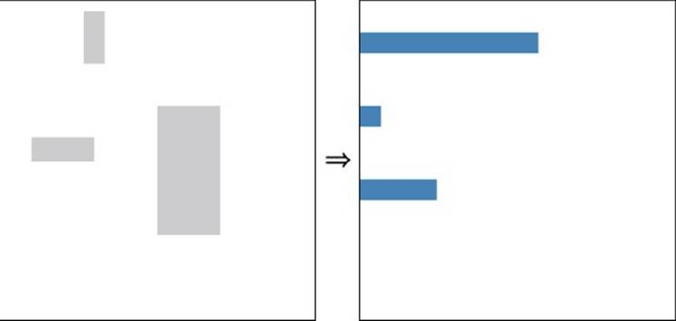
Figure 11.8 The three rectangles that were bound to data and sized accordingly.
Enter
In the previous example there were, conveniently, exactly as many data points as rectangles on the screen. Had there been more data points, they would not have found a rectangle to represent them and would have not been visible. Those points need to “enter” the scene by creating new elements to represent them. (The following code is in the data-enter/script.js file in the Chapter 11 code download on the companion website.)
var svg = d3.select("svg")
var selection = svg.selectAll("rect")
.data([170, 20, 73, 50])
selection
.attr("x", 0)
.attr("y", function(d, i) { return i * 70 + 30 })
.attr("width", function(d) { return d })
.attr("height", 20)
.style("fill", "steelblue")
selection.enter().append("rect")
.attr("x", 200)
.attr("y", 100)
.attr("width", 30)
.attr("height", 30)
.style("fill", "red")
By adding more data than there are elements you are forcing the unmatched datum (50 in this case) to be placed in the enter selection (accessible with selection.enter()).
NOTE Because selections contain elements, the return value of the .enter() function is actually a pseudo-selection as it contains placeholders where the elements will be added. It only becomes a selection when .append is called on it. As a result.enter().append(...) are always called one after the other. The new elements created by the .append are attached as children of the element of the parent selection; in this case it is the svg element.
As shown in Figure 11.9 the extra datum is now represented by the square off to the side, although it is probably not the final result you want. It would be better if the new element followed the same display rules as the existing elements. To achieve that, you could copy the declarative statements
.attr("x", 0)
.attr("y", function(d, i) { return i * 70 + 30 })
.attr("width", function(d) { return d })
.attr("height", 20)
.style("fill", "steelblue")
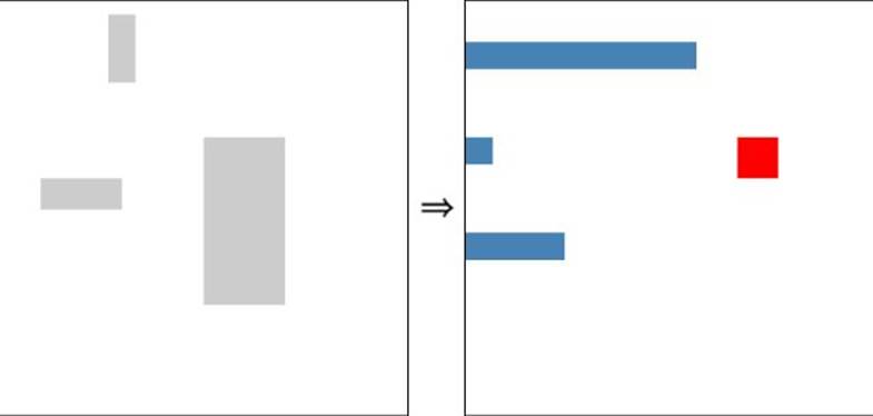
Figure 11.9 The extra datum has been added, but it needs to be restyled.
to the enter selection, but because this is such a common use case and repeating code is a bad idea, D3 provides a shortcut:
var svg = d3.select("svg")
var selection = svg.selectAll("rect")
.data([170, 20, 73, 50])
selection.enter().append("rect")
selection
.attr("x", 0)
.attr("y", function(d, i) { return i * 70 + 30 })
.attr("width", function(d) { return d })
.attr("height", 20)
.style("fill", "steelblue")
Look in the data-enter-shortcut/script.js file in the Chapter 11 download for this code.
Figure 11.10 shows the new element positioned and styled by the declarations on the update selection.
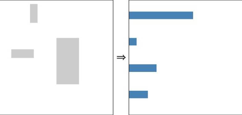
Figure 11.10 The new element matches the existing elements.
By calling .enter().append() you are telling D3 that you want new data elements to be added to the visualization. Doing this before making any updates ensures that the same changes will be applied to both existing (matched by the initial selection) and new elements (created with .enter().append()). If for some reason you wanted to apply some changes to the existing elements and not to the new elements you would have to make your updates before calling .enter().append(). This is highly unusual, so make sure you know why you are doing it.
All previous examples start with an existing svg element within which some number of rectangles are arbitrarily positioned. The purpose of these examples is to showcase selections, and they aren't realistic. In practice, you will likely start from a blank container (probably an HTML <div>) within some page. The first step would then be to append an SVG and start creating elements from scratch.
Applying the previously presented logic to an example without an existing SVG, you get the following, which you can find in the data-enter-blank/script.js file on the companion website:
var svg = d3.select("body").append("svg")
var selection = svg.selectAll("rect")
.data([170, 20, 73, 50])
selection.enter().append("rect")
selection
.attr("x", 0)
.attr("y", function(d, i) { return i * 70 + 30 })
.attr("width", function(d) { return d })
.attr("height", 20)
.style("fill", "steelblue")
Because there is no <svg> to start with, you had to first append it to the visualization container (which in this case is just the <body> element) with d3.select("body").append("svg"). Otherwise, the code is nearly identical to the previous example:
· Start off by selecting all the <rect> elements (of which there are none).
· Compute the data join.
· Put all four data points into the enter selection, which you position and style.
Figure 11.11 shows the bars (and the containing SVG) being created.

Figure 11.11 The bars and the containing SVG are created.
The following is a common pattern that you should be aware of when you browse D3 examples. This code is in the data-enter-pattern/script.js file of the Chapter 11 code downloads.
var someData = [170, 20, 73, 50]
var svg = d3.select("body").append("svg")
svg.selectAll(".bar").data(someData)
.enter().append("rect")
.attr("class", "bar")
.attr("x", 0)
.attr("y", function(d, i) { return i * 70 + 30 })
.attr("width", function(d) { return d })
.attr("height", 20)
.style("fill", "steelblue")
This code pattern is often used when the elements are added only once to a container that is known to be blank. This pattern would produce the same result as Figure 11.6. There is nothing in this code that you have not seen before, but it tends to trip up people who are new to D3.
Because the <svg> element was just created, it must be empty. As a result, calling
svg.selectAll(".bar").data(someData)
is guaranteed to produce an empty update selection that places all the elements into the enter selection. This allows you to ignore the update selection by not assigning it to a variable; instead, you go straight to .enter() to append all of the elements.
Even though the code uses .selectAll(".bar"), because there are no elements yet, it will match nothing and create an empty selection. This means you could technically select anything with the same result; in general you should selectAll using the same selectors that you apply in the append. It should also be noted that although .select(".bar")would also create an empty selection, the data join only works on a selection created with a selectAll. The reasons for this are of little consequence.
Exit
The opposite of having more data than visible elements is having too many elements that must then be removed from the screen. The elements that could not be matched to data are placed into the exit selection and can be instantaneously removed by calling.remove() on that selection.
If you only ever add elements to an empty container based to data that will not change, you won't encounter a meaningful exit selection. If, however, the displayed data changes from user interaction or with the passage of time then you will likely need to remove the elements that are no longer represented by any data after an update.
Enter/Update/Exit
The following general dynamic example (which is on the companion website as data-general/script.js) puts these elements together:
var svg = d3.select("body").append("svg")
function updateBars(barData) {
var selection = svg.selectAll(".bar")
.data(barData)
selection.enter().append("rect")
.attr("class", "bar")
.attr("x", 0)
.attr("height", 20)
.style("fill", "steelblue")
selection
.attr("y", function(d, i) { return i * 70 + 30 })
.attr("width", function(d) { return d })
selection.exit().remove()
}
updateBars([170, 20, 73]) // step 1
updateBars([34, 100]) // step 2
updateBars([100, 34, 150, 160]) // step 3
The example starts with an empty page and appends an <svg> element.
The general enter/update/exit code is wrapped in a function updateBars that can be called repeatedly to update the bars on the screen with the contents of barData.
For clarity and efficiency, you declare all the properties that will never change during the lifetime of the bar on the enter selection and never restate them in the update. In the update selection, you restate the data-driven properties for the updating elements as well as for the freshly created elements added from the enter selection.
As shown in Figure 11.12, in Step 1, three bars are created. Step 2 causes the removal of one bar and an update of the two remaining bars. Step 3 tries to represent four data points, causing two bars to be entered.
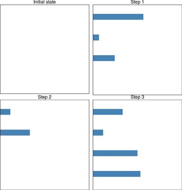
Figure 11.12 Three steps take you from a blank initial state to bars for four data points.
It should be noted that, since D3 always leaves the selection in a consistent state, the previous example did not need to create a new selection on every function run. The example could have instead reused the previous selection with the initial selection being the only one that needed to be created:
var svg = d3.select("body").append("svg")
var selection = svg.selectAll(".bar")
function updateBars(barData) {
var selection = selection.data(barData)
selection.enter().append("rect")
.attr("class", "bar")
.attr("x", 0)
.attr("height", 20)
.style("fill", "steelblue")
selection
.attr("y", function(d, i) { return i * 70 + 30 })
.attr("width", function(d) { return d })
selection.exit().remove()
}
The selection reference would still need to be updated after every .data() call as it creates a new selection. This would be a more efficient than the original example but would only work if the container selection (svg in this case) isn't being dynamically updated.
A More Complex Example
This section provides a slightly more complex example to illustrate some more interesting facets of working with enter/update/exit.
The example develops a top trend viewer. Imagine that there is some application programming interface (API) that can provide an updating top ranking for a given trend. The data provided by this API might look something like this:
var trends1 = [
{ trend: 'Cats', score: 1.0 },
{ trend: 'Dogs', score: 0.8 },
{ trend: 'Fish', score: 0.4 },
{ trend: 'Ants', score: 0.3 },
{ trend: 'Koalas', score: 0.2 }
]
var trends2 = [
{ trend: 'Dogs', score: 1.0 },
{ trend: 'Cats', score: 0.9 },
{ trend: 'Koalas', score: 0.5 },
{ trend: 'Frogs', score: 0.3 },
{ trend: 'Bats', score: 0.2 }
]
// Koalas to the Max!
var trends3 = [
{ trend: 'Koalas', score: 1.0 },
{ trend: 'Dogs', score: 0.8 },
{ trend: 'Cats', score: 0.6 },
{ trend: 'Goats', score: 0.3 },
{ trend: 'Frogs', score: 0.2 }
]
You can find the preceding code and the next code block in the trends-no-join/data.js file in the Chapter 11 download.
This data is composed of an array of trends that each have a trend and a score representing the relative popularity of the trend at a given time. Note that the score of the trend can change from update to update.
var svg = d3.select("body").append("svg")
function updateTrends(trendData) {
var selection = svg.selectAll("g.trend")
.data(trendData)
// enter
var enterSelection = selection.enter().append("g")
.attr("class", "trend")
enterSelection.append("text")
.attr("class", "trend-label")
.attr("text-anchor", "end")
.attr("dx", "-0.5em")
.attr("dy", "1em")
.attr("x", 100)
enterSelection.append("rect")
.attr("class", "score")
.attr("x", 100)
.attr("height", 20)
// update
selection
.attr("transform", function(d, i) {
return "translate(0," + (i * 30 + 20) + ")"
})
selection.select(".trend-label")
.text(function(d) { return d.trend })
selection.select(".score")
.attr("width", function(d) { return d.score * 90 })
// exit
selection.exit().remove()
}
updateTrends(trends1)
updateTrends(trends2)
updateTrends(trends3)
This example showcases some important details:
· Unlike HTML, where nearly every element can contain other elements in SVG, only the g element (g stands for group) can act as a container. Each g element defines its own coordinate system. Finally, g elements cannot be positioned with x, y attributes; they can only be transformed with the transform attribute.
· After elements are appended to the pseudo-selection returned by .enter(), you get a regular selection (assigned to enterSelection) to which you can append more elements. enterSelection.append("text") adds a single <text> element to every entered g and returns a selection of those text elements, allowing you to configure them. Note that this example would not work if all the appends were simply chained to each other because every append returns a new selection (it would put the <rect> elements into the <text>elements, which is invalid). The solution is to save a reference to enterSelection and append twice on it.
· The text position is fine tuned using dx and dy attributes. Those are added by the renderer to the x and y attributes respectively and can be specified relative to the text font size (with the em unit). Setting .attr("dy", "1em") effectively lowers the text by one line height.
· In the update selection, which comprises g.trend elements, you can select the trend labels using selection.select(".trend-label") to apply the updated trend name to them. The datum bound to the trend labels is inherited from its container by default.
The output of this example is shown in Figure 11.13.
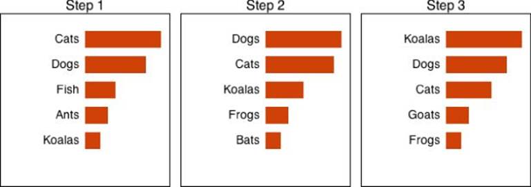
Figure 11.13 These steps show the trend bars at three points in time.
Key Functions
The final (and most important) aspect of D3's data join principle is the key function. This section examines how to specify which data points map to which visual elements and why it is so important.
The key function can be provided as the second argument to the .data() function and should map a given datum to a string (key) that will be used to identify the element. The key function will be run both on the data bound to the elements in the existing selection and the new data given to the .data() function. Any elements whose key matches a data key is placed in the update selection.
You can improve the previous example with a small tweak. The code for the following example is in the trends-join/script.js in the Chapter 11 download.
var svg = d3.select("body").append("svg")
function updateTrends(trendData) {
var selection = svg.selectAll("g.trend")
.data(trendData, function(d) { return d.trend })
// enter
var enterSelection = selection.enter().append("g")
.attr("class", "trend")
enterSelection.append("text")
.attr("class", "trend-label")
.attr("text-anchor", "end")
.attr("dx", "-0.5em")
.attr("dy", "1em")
.attr("x", 100)
.text(function(d) { return d.trend })
enterSelection.append("rect")
.attr("class", "score")
.attr("x", 100)
.attr("height", 20)
// update
Selection
.attr("transform", function(d, i) {
return "translate(0," + (i * 30 + 20) + ")"
})
selection.select(".score")
.attr("width", function(d) { return d.score * 90 })
// exit
selection.exit().remove()
}
updateTrends(trends1)
updateTrends(trends2)
updateTrends(trends3)
The changes are very subtle (and invisible, refer to Figure 11.13) but their effect is profound.
By default, the join is done using the index of the datum. Writing .data(trendData) is equivalent to writing .data(trendData, function(d, i) { return String(i) }). This means that the first <g> element would have bound to the Cats trend in Step 1, the Dogs trend in Step 2, and the Koalas trend in Step 3. As a result, the text of the <text> element needed to be continuously updated.
In the updated example, the data join is done according to the trend property of the data (function(d) { return d.trend }). Thus the first <g> element stays bound to the Cats trend forever. You utilize this by setting the text of the <text> element only once, when creating the elements.
It is very important to define the key function in a way that represents the essence of the data. This is helpful for not having to update labels. Most of all, though, this is critical to getting element transitions to look accurate.
.transition()
The ability to show transitions is a huge advantage of dynamic media—such as the web—over static media.
Transitions are often used in one of the following contexts:
· To visualize data changing over time: One way to represent time in the data is to vary the visual elements with time. This is typically called animation.
· To preserve object constancy within a visualization: When the positions of the visual elements change based on user interaction, having the elements smoothly transition makes it easier for the viewer to track the change. An example of this would be if, in a bar chart, the user could change the order of the bars.
· To preserve object constancy between visualizations: When the visualization can trans-morph into a different visualization it is particularly helpful for the individual elements to transition into their new shape.
· To add visual flare to the visualization: Transitions can add polish to a visualization and, if used with discretion, can make it appear more refined.
For a detailed analysis of the merits of different kinds of transitions, refer to “Animated Transitions in Statistical Data Graphics” by Jeff Heer and George Robertson, which you can find at http://vis.stanford.edu/papers/animated-transitions.
D3 is incredibly powerful at expressing transitions with a high degree of customization, which makes it a great choice for dynamic visualizations.
A Basic Transition
Try applying some transitions to a single circle (see the transition-basic/script.js file in the code download for Chapter 11):
var svg = d3.select("body").append("svg")
svg.append("circle")
.attr("cx", 20)
.attr("cy", 20)
.attr("r", 10)
.style("fill", "gray")
.transition()
.delay(300)
.duration(700)
.attr("cx", 150)
.attr("cy", 100)
.attr("r", 40)
.style("fill", "#FFC000")
.transition()
.duration(1000)
.attr("cx", 130)
.attr("cy", 250)
.attr("r", 20)
.style("fill", "red")
.attr("opacity", 1)
.transition()
.duration(1000)
.attr("opacity", 0)
.remove()
NOTE The general convention of D3 code is to add indentation every time the return value is a new selection.
The snapshots of this transition at key points are shown in Figure 11.14. To get the full experience, you should run this example yourself; it's in the transition-basic/index.html file.
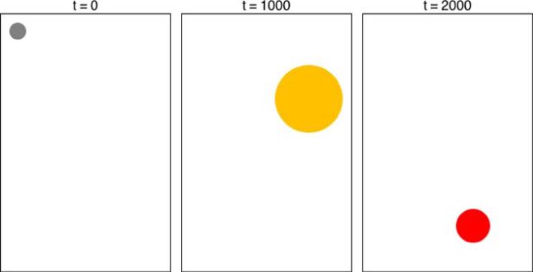
Figure 11.14 The circle animation is shown in three snapshots.
There are some important features demonstrated in this example that highlight the immense power and expressibility of the D3 API.
For simplicity, you append a single gray circle like so:
svg.append("circle")
.attr("cx", 20)
.attr("cy", 20)
.attr("r", 10)
.style("fill", "gray")
By calling .transition() on this single element selection, you create a new type of selection called the transition selection (hence the indentation). The transition selection behaves like a regular selection except that the properties defined on it refer to the end state of the transition as opposed to setting the immediate state.
.delay(300)
.duration(700)
.attr("cx", 150)
.attr("cy", 100)
.attr("r", 40)
.style("fill", "#6")
You can also specify how long the transition will take (700ms in this case) and how long it will delay before starting (300ms). You define the end state and let D3 take care of the rest. Notice that despite using a named color "gray" in the starting state and a hex color"#FFC000" in the ending state, D3 is able to interpolate between them.
But wait, there's more!
.transition()
.duration(1000)
.attr("cx", 130)
.attr("cy", 250)
.attr("r", 20)
.style("fill", "red")
.attr("opacity", 1)
Simple transitions can be chained to form complex multistage transitions. Each transition in the chain starts after the previous one is finished.
Notice the tag on an explicit declaration for .attr("opacity", 1) (opacity is 1 by default). This prepares your trusty circle for its grand finale:
.transition()
.duration(1000)
.attr("opacity", 0)
You declare one final transition where you tell the circle to fade out over the course of one second. You needed to set opacity to 1 explicitly first because D3 cannot interpolate an attribute that is not defined (even if there is an implicit default). Finally, you call.remove() on the last transition selection. This tells D3 to remove all the elements in the selection when the transition completes.
This circle existed for a total of three seconds and yet it has taught us so much.
Object Constancy
Now that you have seen how easy it is to transition the elements of a selection, you can revisit the trends example to see how transitions can enhance the visualization. A primary application of transitions is to maintain object constancy between the trends, allowing the viewer's eye to easily follow how trends change their rank. You can also add a nice fade in/out effect for arriving and departing trends for a bit of artistic flourish. (Refer to the trends-transition/script.js file.)
var svg = d3.select("body").append("svg")
function updateTrends(trendData) {
var selection = svg.selectAll("g.trend")
.data(trendData, function(d) { return d.trend })
// enter
var enterSelection = selection.enter().append("g")
.attr("class", "trend")
.attr("opacity", 0)
.attr("transform", function(d, i) {
return "translate(0," + (i * 30 + 20) + ")"
})
enterSelection.append("text")
.attr("class", "trend-label")
.attr("text-anchor", "end")
.attr("dx", "-0.5em")
.attr("dy", "1em")
.attr("x", 100)
.text(function(d) { return d.trend })
enterSelection.append("rect")
.attr("class", "score")
.attr("x", 100)
.attr("height", 20)
.attr("width", 0)
// update
Selection
.transition()
.delay(1200)
.duration(1200)
.attr("opacity", 1)
.attr("transform", function(d, i) {
return "translate(0," + (i * 30 + 20) + ")"
})
selection.select(".score")
.transition()
.duration(1200)
.attr("width", function(d) { return d.score * 90 })
// exit
selection.exit()
.transition()
.ease("cubic-out")
.duration(1200)
.attr("transform", function(d, i) {
return "translate(200," + (i * 30 + 20) + ")"
})
.attr("opacity", 0)
.remove()
}
updateTrends(trends1)
setTimeout(function() {
updateTrends(trends2)
}, 4000)
setTimeout(function() {
updateTrends(trends3)
}, 8000)
This example really needs to be seen in action to be fully understood. Please run it yourself using the trends-transition/step3.html file.
Examine the enter, update, and exit parts of this transition individually:
· The entering <g> elements have their opacity set to 0, making them invisible. Their initial position is set using the same logical mapping as what they will later transition to when they join the update selection.
· The update selection is transitioned over a period of 1200ms (with a 1200ms delay to let the exit transition finish). The end-state opacity is set to 1 to get the elements joining in from the enter selection to fade in (this has no effect on the elements that were already on the screen as their opacity was already 1). The transform is updated to reflect the new position given the (potentially new) rank of the trend.
· The exiting <g> elements, whose trends are no longer in the top five, are transitioned 200px to the right and faded out. They use the cubic-out easing function to make the transition look more natural. After the transition is finished, they are removed.
This example clearly shows the importance of defining the key function correctly. Without it, these transitions would not look right as the same five elements would simply be recycled to represent the new trends. There would never be a non-empty exit selection and thus no place to specify how the no-longer-top-five trends bid their farewell.
An interesting behavior to note is that because the elements in the exit selection were, by definition, not joined with a new data they end up keeping their (old) bound data value until they are removed. Any operand modification on the exit selection will act on the last data bound to that element.
The key function should never translate two distinct data objects into the same key. Doing so would lead to undefined behavior and strange errors. You need not worry about overlapping keys if you are not defining a key function because the default key function is to key a datum by its index.
Nested Selections
The final point of awesomeness about selections is that they can be nested, allowing you to effectively represent nested data structures that occur so often in data visualization.
Consider the following data structure representing a 4x4 matrix:
var matrixData = [
[9.4, 2.8, 2.3, 6.3],
[5.3, 6.3, 7.7, 4.7],
[6.1, 7.3, 7.9, 0.8],
[1.2, 2.6, 7.3, 2.6]
]
It is an array representing the rows where each row is, itself, an array representing the cells of the matrix. Say you wanted to visualize this by rendering the numbers in a grid; you could break down the visualization into two conceptual parts: rendering an array of numbers into a row and rendering the array of rows to form a grid. These two steps can be tackled independently by making use of nested selections. First you can create a selection of rows and associate the data for individual rows with each row element. Because a row element contains other elements in it (for numbers) you must use a group element (<g>) because it is the only SVG container element. Next within each row group you create a selection of elements that represent the individual numbers. Because each number will be represented as a circle and some text, those can also be grouped together.
var svg = d3.select("body").append("svg")
// First selection (rows)
var rowSelection = svg.selectAll("g.row").data(matrixData)
rowSelection.exit().remove()
rowSelection.enter().append("g")
.attr("class", "row")
.attr("transform", function(d, i) {
return "translate(0," + (i * 45 + 30) + ")"
})
// Second selection (cells)
var cellSelection = rowSelection
.selectAll("g.cell").data(function(d) { return d })
cellSelection.exit().remove()
var enterCellSelection = cellSelection.enter().append("g")
.attr("class", "cell")
.attr("transform", function(d, i) {
return "translate(" + (i * 45 + 30) + ",0)"
})
// Fill in the cells
enterCellSelection.append("circle")
.attr("r", function(d) { return Math.sqrt(d * 140 / Math.PI) })
enterCellSelection.append("text")
.attr("text-anchor", "middle")
.attr("dy", "0.35em")
.text(function(d) { return "[" + d + "]" })
You can find the preceding code in the nested-simple/script.js file in the Chapter 11 download.
You create a selection of g.row and associate matrixData with it. Because matrixData is an array of arrays, the data element being associated with each g.row is itself an array. Note that in the example the steps are rearranged, with exit first for better readability.
Next, you use the nested capabilities of D3 selections to create a selection within each g.row element. All examples shown previously had only one element (usually the SVG container) in the selection on which you performed a data join. In contrast, the second data join in this example is performed on a selection that already has four elements (g.row) in it, each with its own data. In this data join, .selectAll("g.cell").data(function(d) { return d }), the first argument to the data operator is a function that defines the data to be used in the join within each of the row groups. The trivial function supplied simply returns the row array, causing D3 to create an element for each number in the row (within each row). You use a group (g.cell) to represent each number within the row so that both the text and circle elements appear in the same place.
Finally, you fill each g.cell with a circle (circle) and a label (text). At this point the data associated with each g.cell element is the corresponding number of the matrix so calling
enterCellSelection.append("circle")
.attr("r", function(d) { return Math.sqrt(d * 140 / Math.PI) })
creates a circle and sets its radius in such a way as to make its area equal to d * 140. You can see the resulting bubble matrix in Figure 11.15.
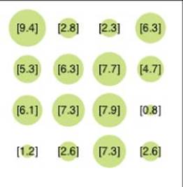
Figure 11.15 The result is a bubble matrix.
D3 Helper Functions
The big advantage of D3 is that, after you understand the data join principle and transitions described earlier in this chapter, you are set; other visualization toolkits typically have under-the-covers “magic” that makes is very easy to start using them but hard to understand what is actually going on behind the scenes. In D3 you get the powerful data joins and transitions, the rest you need to provide yourself. Helpfully D3 comes packed with many independent, self-contained function generators that can be of use in a number of scenarios to simplify the task of creating complex visualizations. Most D3 helper functions can be used in contexts completely outside of D3 as they have nothing D3 specific about them.
This section examines some of the most popular helper functions.
Drawing Lines
Line charts are a staple of visualization. Unfortunately, drawing lines in SVG is a pain, as shown here (see the helper-line-raw/script.js file in the code downloads):
var svg = d3.select("body").append("svg")
svg.append("path")
.style("fill", "none")
.style("stroke", "black")
.style("stroke-width", 2)
.attr("d", "M10,10L100,100L100,200L150,50L200,75")
To draw a line, you need to set the d attribute of a <path> element to a string of M (move) and L (line) commands. D3 has a helper function so that you never have to deal with these crazy strings yourself (see the helper-line/script.js file in the Chapter 11 code download):
var points = [
{ x: 10, y: 10 },
{ x: 100, y: 100 },
{ x: 100, y: 200 },
{ x: 150, y: 50 },
{ x: 200, y: 75 }
]
var lineFn = d3.svg.line()
.x(function(d) { return d.x })
.y(function(d) { return d.y })
var svg = d3.select("body").append("svg")
console.log(lineFn(points))
// => "M10,10L100,100L100,200L150,50L200,75"
svg.append("path")
.style("fill", "none")
.style("stroke", "black")
.style("stroke-width", 2)
.attr("d", lineFn(points))
Calling d3.svg.line() returns a function that, when called on an array of data, produces an SVG path string. This function lives within the d3.svg namespace to indicate that it is SVG specific. The results of both of these examples are identical (see Figure 11.16).

Figure 11.16 A path element drawing a polyline
D3's API style makes heavy use of function chaining. The d3.svg.line() helper can be configured to correctly extract the x and y coordinates from the data by using the .x(...) and .y(...) setter methods respectively:
.x(function(d) { return d.x })
.y(function(d) { return d.y })
The preceding code tells the line helper to use d.x and d.y as the coordinates of the points.
Scales
A scale is a function that maps from an input domain to an output range. Scales find their way into nearly every visualization as you often need to do a transformation to convert data values to pixel sizes.
D3 provides a number of different scales to suit different types of data:
· Quantitative scales are used for continuous input domains, such as numbers.
· Time scales are quantitative scales specifically tuned to time data.
· Ordinal scales work on discrete input domains, such as names or categories.
In the previous bar chart–based examples, the bars were always horizontal. Because of the location of the origin in the SVG coordinate system, horizontal bar charts are simpler to describe compared to the more traditional vertical bar charts.
You can create a vertical bar chart with the help of two scales. You can find the following code in the helper-scales/script.js file.
var svg = d3.select("body").append("svg")
function updateGdpBars(gdpData, width, height) {
var countries = gdpData.map(function(d) { return d.country })
var xScale = d3.scale.ordinal()
.domain(countries)
.rangeBands([0, width], 0.2)
var maxGdp = d3.max(gdpData, function(d) { return d.gdp })
var yScale = d3.scale.linear()
.domain([0, maxGdp])
.range([height - 20, 20])
var selection = svg.selectAll(".bar")
.data(gdpData)
selection.enter().append("rect")
.attr("class", "bar")
.style("fill", "steelblue")
Selection
.attr("x", function(d) { return xScale(d.country) })
.attr("y", function(d) { return yScale(d.gdp) })
.attr("width", xScale.rangeBand())
.attr("height", function(d) {
return Math.abs(yScale(d.gdp) - yScale(0))
})
selection.exit().remove()
}
var UN_2012_GDP = [
{ country: "United States", gdp: 16244600 },
{ country: "China", gdp: 8358400 },
{ country: "Japan", gdp: 5960180 },
{ country: "Germany", gdp: 3425956 },
{ country: "France", gdp: 2611221 },
{ country: "United Kingdom", gdp: 2471600 }
]
updateGdpBars(UN_2012_GDP, 600, 300)
The example shown in Figure 11.17 is much closer to what you might encounter in the wild.

Figure 11.17 The bars have been redrawn with a vertical orientation.
You create two scales, xScale and yScale, for the x and y axes respectively.
var countries = gdpData.map(function(d) { return d.country })
var xScale = d3.scale.ordinal()
.domain(countries)
.rangeBands([0, width], 0.2)
The input domain of the xScale is the list of countries (countries). Because this is an ordered list of discrete values, you use the d3.scale.ordinal() scale. You ask the scale to map these values onto a range of [0, width], splitting them into equal bands with 20 percent of the space used as a gap. Later, you will access the width of a single bar using the xScale.rangeBand() method.
var maxGdp = d3.max(gdpData, function(d) { return d.gdp })
var yScale = d3.scale.linear()
.domain([0, maxGdp])
.range([height - 20, 20])
For the y axis you use a d3.scale.linear() scale. This scale creates a simple linear function of the form y = m*x + c for some m and c. You use another helper function, d3.max, to find the maximum gdp within the data.
In many D3 examples, the x and y scales are stored in variables called x and y. This sometimes trips up beginners as people are used to variables x and y being numeric (as opposed to functions).
You position the bars as needed using
selection
.attr("x", function(d) { return xScale(d.country) })
.attr("y", function(d) { return yScale(d.gdp) })
.attr("width", xScale.rangeBand())
.attr("height", function(d) {
return Math.abs(yScale(d.gdp) - yScale(0))
})
The x and y attributes are determined by using the scales directly. The width is determined from the band size conveniently provided by the ordinal scale. You compute the height by subtracting the value of the scale at the given data value from the scale value at zero.
D3 Helper Layouts
Another type of helper function provided by D3 is layouts. Unlike the helper functions discussed previously, which help you map data to attribute values, layouts work on the data, augmenting it with more information.
A treemap is a popular visualization that recursively subdivides area into rectangles sized according to some data attribute. You can easily create treemaps with the aid of the d3.layout.treemap() layout, which does all the complex computations for you.
Treemaps were introduced by Ben Shneiderman in 1991. You can read more about them at http://www.cs.umd.edu/hcil/treemap-history/.
You can see how the treemap layout can be used in practice by applying it to the problem it was originally designed to solve: visualizing the file sizes/hierarchy on a disk drive. You apply the treemap layout to the file structure within the example folder for this chapter.
var FILE_DATA = {
"name": "examples",
"content": [
{
"name": "blank",
"content": [
{
"name": "index.html",
"size": 320
}
]
},
{
"name": "data-enter",
"content": [
{
"name": "after.html",
"size": 512
},
{
"name": "before.html",
"size": 475
},
{
"name": "script.js",
"size": 404
}
]
}
...lots of data omitted...
]
}
This is the data to be used in this example. As you can see, it is hierarchical as it describes a file system. (Refer to the layout-treemap/script.js file in the code downloads.)
var svg = d3.select("body").append("svg")
function updateTreemap(fileData, width, height) {
var treemap = d3.layout.treemap()
.size([width, height])
.children(function(d) { return d.content })
.value(function(d) { return d.size })
var nodeData = treemap.nodes(fileData)
var color = d3.scale.category20c()
var selection = svg.selectAll("g.node")
.data(nodeData)
// Exit
selection.exit().remove()
// Enter
enterSelection = selection.enter().append("g")
.attr("class", "node")
enterSelection.append('rect')
enterSelection.append('text')
.attr('dx', '0.2em')
.attr('dy', '1em')
// Update
selection
.attr("transform", function(d) { return "translate(" + d.x + "," + d.y + ")" })
selection.select('rect')
.attr("width", function(d) { return d.dx })
.attr("height", function(d) { return d.dy })
.style("stroke", 'black')
.style("fill", function(d) { return d.children ? color(d.name) : 'none' })
selection.select('text')
.text(function(d) {
if (d.children || d.dx < 50 || d.dy < 10) return null
return d.name
})
}
updateTreemap(FILE_DATA, 700, 400)
Start off by declaring the layout:
var treemap = d3.layout.treemap()
.size([width, height])
.children(function(d) { return d.content })
.value(function(d) { return d.size })
You set the container dimensions (size), the child node accessor (children), and the value function (value). These tell the layout how to traverse the hierarchy of the data.
Each layout, by convention, provides a nodes and a links function for generating the nodes that correspond to the data and the links that represent their interconnections.
var nodeData = treemap.nodes(fileData)
For the treemap, you are only interested in the nodes. You run the data through the nodes function and get back a flat array representing the rectangles of the treemap with lots of useful metadata attached.
Here is what an element of nodeData looks like:
{
name: "data-general"
area: 15716.360529688169
children: Array[8]
content: Array[8]
depth: 1
x: 174
y: 202
dx: 170
dy: 92
parent: Object
value: 1971
}
As you can see, all the original values are preserved, but extra metadata for positioning (x, y, dx, and dy) is added.
You now perform the regular data join onto the new nodeData.
selection
.attr("transform", function(d) { return "translate(" + d.x + "," + d.y + ")" })
selection.select('rect')
.attr("width", function(d) { return d.dx })
.attr("height", function(d) { return d.dy })
You position the container group and size the rectangles using the metadata generated by the layout function.
The resulting treemap is shown in Figure 11.18.
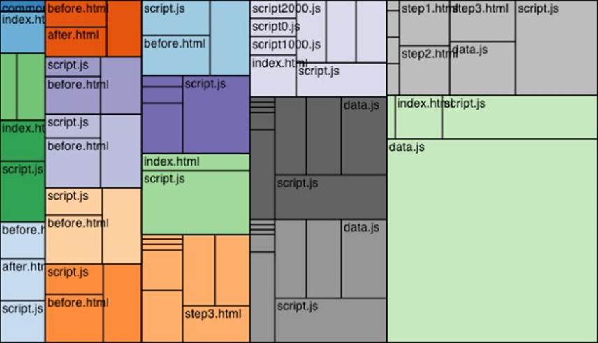
Figure 11.18 This treemap visualizes the files in this chapter scaled by file size.
Summary
This chapter introduced D3 and showcased the core principles that make it up:
· You saw how to select elements and create new elements using D3.
· You found out how to position and style elements using the .attr and .style functions.
· You learned D3's core principle of joining data to elements and the resulting enter, update, and exit selections.
· You saw how transitions work and how they can be chained together.
· You discovered how to fine-tune the joining and maintain constancy by providing a join key function.
· You learned about nesting selections within selections as a means of representing nested data structures.
· You were introduced to the different types of helper functions provided by D3 that aid in creating visualizations:
· You learned about scales that help you transform values from the data to pixels.
· You found out about layouts that reshape your data to make it easier to work with.
All materials on the site are licensed Creative Commons Attribution-Sharealike 3.0 Unported CC BY-SA 3.0 & GNU Free Documentation License (GFDL)
If you are the copyright holder of any material contained on our site and intend to remove it, please contact our site administrator for approval.
© 2016-2026 All site design rights belong to S.Y.A.