JavaScript and jQuery for Data Analysis and Visualization (2015)

PART IV Interactive Analysis and Visualization Projects

· Chapter 15: Building an Interconnected Dashboard

· Chapter 16: Building Interactive Infographics with D3

Chapter 15 Building an Interconnected Dashboard

What's In This Chapter

· Pulling data from the U.S. Census API

· Rendering Census data with Google Charts

· Styling the chart dashboard responsively

· Connecting the components with Backbone

CODE DOWNLOAD The wrox.com code downloads for this chapter are found at www.wrox.com/go/javascriptandjqueryanalysis on the Download Code tab. The code is in the chapter 15 download and individually named according to the names throughout the chapter.

With this chapter, you create an interactive dashboard that charts U.S. census data. You start by exploring the Census API and learn how to overcome its many challenges. Next you render static charts from this data using Google Charts. You create visualizations for a variety of data:

· Demographic data for sex and race

· Housing data

· Population growth and age breakdowns

After creating the charts, you then integrate them into an interconnected dashboard. You start by styling the dashboard responsively and then integrate form controls to translate user input into rendered changes on the screen. In the end, you'll have created a simple Backbone app that renders complex data.

The U.S. Census API

In recent years, the U.S. government has been releasing a variety of public APIs for governmental data. Collected at www.data.gov, these APIs provide a variety of useful data sets. Notably, the Census API offers a wealth of intricate demographic information about U.S. residents.

To get started with the API, register for an API key at www.census.gov/developers/. After you're in the site, you see that there are a variety of different data sets available. For now, take a look at the Decennial Census Data:

1. http://www.census.gov/data/developers/data-sets/decennial-census-data.html

A quick word of warning: Working with the Census API can be cumbersome. Rather than using an intuitive data structure, you have to dig through mountains of XML to figure out how to access the desired data.

For example, say you want to figure out simple gender information. The first step is to look in http://api.census.gov/data/2010/sf1/variables.xml for the key for the data you want. In this case, you need P0120002 and P0120026, which are aggregated values for the “sex by age” data for men and women respectively.

Next, include these keys along with your API key in a call to the API:

http://api.census.gov/data/2010/sf1?get=

P0120002,P0120026&for=state:*&key=[your_api_key]

For now, just paste this link in your browser. If your API key is working, you should see this data:

[["P0120002","P0120026","state"],

["2320188","2459548","01"],

["369628","340603","02"],

["3175823","3216194","04"],

["1431637","1484281","05"],

...

["287437","276189","56"],

["1785171","1940618","72"]]

That's 2010 census data for men and women broken down by state. For instance, the second line, ["2320188","2459548","01"] represents:

· "2320188": The number of men (P0120002)

· "2459548": The number of women (P0120026)

· "01": In Alabama

The final value, 01, is the FIPS (Federal Information Processing Standards) state code for Alabama. Unfortunately, you can't query the Census API using intuitive strings such as men, women, and Alabama; instead, you have to use random government codes such asP0120002, P0120026, and 01.

TIP For a list of FIPS state codes, visit http://en.wikipedia.org/wiki/Federal_Information_Processing_Standard_state_code.

The previous example pulls a list for all states, but you can also specify a given state using the FIPS state code. For example, to pull the information for only Alabama, you'd call

http://api.census.gov/data/2010/sf1?get=P0120002,P0120026&for=state:01

&key=[your_api_key].

That returns a much smaller data set:

[["P0120002","P0120026","state"],

["2320188","2459548","01"]]

TIP USA Today provides a more intuitive API for census data at http://developer.usatoday.com/docs/read/Census. It's handy for simple data, but not nearly as powerful as the API from www.census.gov.

Rendering Charts

Now that you have data from the census API, rendering it in a chart will be a piece of cake. To keep things simple, you're going use Google Charts and just hardcode the charts for a specific state (New York). Then, later in this chapter you integrate these components into an interactive Backbone app that works for all 50 states in the United States.

Sex Chart

First, let's create a chart using the male versus female demographic information you accessed earlier. To get started, grab the data using jQuery's ajax() API:

$.ajax({

url: "http://api.census.gov/data/2010/sf1",

data: {

get: "P0120002,P0120026",

for: "state:36",

key: "[your API key]"

success: function(data) {

console.log(data);

}

});

This snippet reformats the query to api.census.gov, breaking out the query variables into the data object. After you've entered your API key, you should see the console outputting the sex data you accessed earlier.

Next, display this data in a chart. First include a wrapper for the chart, the Google JS API, and load the chart's API:

google.load("visualization", "1", {packages:["corechart"]});

google.setOnLoadCallback(renderCharts);

</script>

Now, the API calls renderCharts() whenever the chart scripts load. Add the Ajax call to api.census.gov to this callback, and render the chart:

function renderCharts() {

$.ajax({

url: "http://api.census.gov/data/2010/sf1",

data: {

get: "P0120002,P0120026",

for: "state:36",

key: "[your API key]"

success: function(data) {

var processed = [

["Sex", "Population"],

["Male", ∼∼data[1][0]],

["Female", ∼∼data[1][1]]

];

var chartData = google.visualization.arrayToDataTable(processed);

var options = {

title: "Sex",

pieHole: 0.8,

pieSliceText: "none"

};

var chart = new google.visualization.PieChart(

document.getElementById("sex-chart")

);

chart.draw(chartData, options);

}

});

}

In the success callback, you see a bit of data massaging to convert the raw census data to the format Google Charts expects. In defining the processed variable, you first include an array to name the columns of the chart and then pass in each row of data. For each row, you simply pull the relevant value from the Census API data and then convert it to an integer using the ∼∼ literal.

NOTE The ∼∼ literal is similar to Math.floor, except with better performance.

The script next creates an options object for Google Charts, setting some basic options, along with pieHole to render the donut chart in Figure 15.1.

NOTE You can find this example in the Chapter 15 folder on the companion website. It's named sex-chart.html.

c15fig001

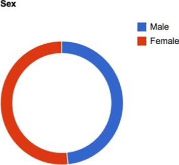
Figure 15.1 This chart shows sex demographics in New York.

Race Chart

You can now take a similar approach to create a chart for race demographics. When working with the Census API, the first step is hunting down just what keys you want to pull from the data set. In this case, you need to look at the P8. RACE section, in particularP0080003 through P0080009.

Next, you can follow the patterns in the sex chart to render this new chart in the renderCharts() callback:

$.ajax({

url: "http://api.census.gov/data/2010/sf1",

data: {

get: "P0080003,P0080004,P0080005,P0080006,P0080007,P0080008,P0080009",

for: "state:36",

key: "[your API key]"

success: function(data) {

var races = [

"White",

"Black",

"American Indian or Alaskan Native",

"Asian",

"Native Hawaiian or Pacific Islander",

"Other",

"Mixed"

processed = [

["Race", "Population"]

];

// lose the last value (state ID)

data[1].pop();

for ( i in data[1] ) {

processed.push([

races[i],

∼∼data[1][i]

]);

}

var chartData = google.visualization.arrayToDataTable(processed);

var options = {

title: "Race",

is3D: true

};

var chart = new google.visualization.PieChart(

document.getElementById("race-chart")

);

chart.draw(chartData, options);

}

});

Here the code follows the sex chart example for the most part except that it's dealing with more values, so it's a bit easier to loop through these values to create the processed variable. Finally, instead of a donut chart, this data makes more sense to display as a pie chart, so the pieHole in the options has been replaced with is3D to render the 3D pie chart in Figure 15.2.

TIP Make sure to include a wrapper for each chart in the markup, as shown in the example in the Chapter 10 folder on the companion website. It's named race-chart.html. Note that it might render differently based on the size of your screen; Google Charts adds information depending on the size of the chart wrapper.

c15fig002

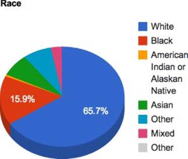
Figure 15.2 Race demographics in New York have been charted.

Household Size Chart

Next let's create a visualization for the information in H13. Household Size, in particular H0130002 through H0130008:

$.ajax({

url: "http://api.census.gov/data/2010/sf1",

data: {

get: "H0130002,H0130003,H0130004,H0130005,H0130006,H0130007,H0130008",

for: "state:36",

key: "[your API key]"

success: function(data) {

var processed = [

["Household Size", "Households"]

];

// lose the last value (state ID)

data[1].pop();

for ( i in data[1] ) {

processed.push([

(∼∼i+1) + ( i == 6 ? "+" : "" ) + " Person",

∼∼data[1][i]

]);

}

var chartData = google.visualization.arrayToDataTable(processed);

var options = {

title: "Household Size",

is3D: true

};

var chart = new google.visualization.PieChart(

document.getElementById("household-chart")

);

chart.draw(chartData, options);

}

});

Here, the script follows the patterns from the race chart almost exactly, with one exception. Rather than hardcoding the name for each key, it generates them dynamically using the loop index to create keys like “1 Person,” “2 Person,” and “7+ Person.” That renders the chart in Figure 15.3.

c15fig003

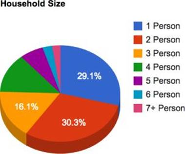
Figure 15.3 This chart shows household sizes in New York.

You can find this example in the Chapter 15 folder on the companion website. It's named household-chart.html.

Household Tenure Chart

Next you create a chart for household tenure data—that is, the percentage of homes that are owned versus rented. This chart is again very simple; this time it follows the basic sex chart example, except with the data in H11. TOTAL POPULATION IN OCCUPIED HOUSING UNITS BY TENURE.

$.ajax({

url: "http://api.census.gov/data/2010/sf1",

data: {

get: "H0110002,H0110003,H0110004",

for: "state:36",

key: "[your API key]"

success: function(data) {

var processed = [

["Tenure", "Housing Units"],

["Owned with Mortgage", ∼∼data[1][0]],

["Owned Outright", ∼∼data[1][1]],

["Rented", ∼∼data[1][2]]

];

var chartData = google.visualization.arrayToDataTable(processed);

var options = {

title: "Housing Tenure",

pieHole: 0.8,

pieSliceText: "none"

};

var chart = new google.visualization.PieChart(

document.getElementById("tenure-chart")

);

chart.draw(chartData, options);

}

});

As you can see, the script simply hardcodes the names for each piece of data and includes the relevant value. The end result is the donut chart in Figure 15.4.

c15fig004

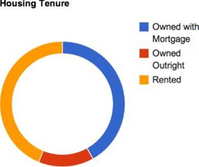
Figure 15.4 This chart shows housing tenure data for New York.

You can find this example in the Chapter 15 folder on the companion website. It's named tenure-chart.html.

Age by Sex Chart

So far you've been working with small data sets. But now it's time to think a bit larger and display a chart showing how the population is dispersed across different ages and genders. For these purposes, you need to leverage the mammoth P12. Sex By Age data set.

Because you're going to be grabbing a lot more data (46 values to be exact), start by creating a function to generate the keys you need:

function build_age_request_string(offset) {

var out = "";

for ( var i = 0; i < 23; i++ ) {

var this_index = ("0" + (i + offset)).slice(-2);

out += "P01200" + this_index + ",";

}

return out;

}

var age_request_keys = build_age_request_string(3) + build_age_request_string(27);

age_request_keys = age_request_keys.slice(0,-1);

Don't get too hung up on this script; it's just a quick piece of code to output the 46 keys you need (P0120003 through P0120025 for men and P0120027 through P0120049 for women).

Next, pass these references into an API call:

$.ajax({

url: "http://api.census.gov/data/2010/sf1",

data: {

get: age_request_keys,

for: "state:36",

key: "[your API key]"

success: function(data) {

var male_data = data[1].slice(0,23),

female_data = data[1].slice(23,46);

}

});

Here the script uses the age_request_keys string you previously generated to pull the data, and then it slices out the male and female data sets from the result. Next, if you look at the Census API reference, notice that these age buckets are not all equal. For the most part, they represent a five-year age range—for example, 5–9 or 10–14—but there are a handful of outliers such as 15–17 and 18–19. In order to build a relevant visualization, it's important to rectify these differences and create useful comparisons.

Fortunately, the unusual age groupings can be merged into the standard five-year buckets:

function combine_vals(arr, start, end) {

var total = 0;

for ( var i = start; i <= end; i++ ) {

total += arr[i];

}

arr[start] = total;

arr.splice( start + 1, end - start);

return arr;

}

function clean_age_range( age_data ) {

// convert all the values to numeric

for ( var i in age_data ) {

age_data[i] = ∼∼age_data[i];

}

// merge values starting with highest (to preserve array keys)

// merge 65-66 && 67-69

age_data = combine_vals( age_data, 17, 18 );

// merge 60-61 & 62-64

age_data = combine_vals( age_data, 15, 16 );

// merge 20, 21 & 22-24

age_data = combine_vals( age_data, 5, 7 );

// merge 15-17 & 18-19

age_data = combine_vals( age_data, 3, 4 );

return age_data;

}

male_data = clean_age_range(male_data);

female_data = clean_age_range(female_data);

Here the script first defines the function combine_vals() for merging array values and then leverages that in the clean_age_range() function, which manually groups the unusual values. Next you can further refine this data to use with Google Charts:

var processed = [

["Age", "Male", "Female"]

];

for ( var i = 0, max = male_data.length; i < max; i++ ) {

var row = [];

switch(i) {

case 0:

row[0] = "Under 5";

break;

default:

row[0] = (i * 5) + "-" + (i * 5 + 4);

break;

case max - 1:

row[0] = (i * 5) + "+";

break;

}

row[1] = male_data[i];

row[2] = female_data[i];

processed.push(row);

}

Here the code simply loops through the age data and outputs a useful name along with the male and female populations. Finally, pass this information into a Google Charts column chart:

var chartData = google.visualization.arrayToDataTable(processed);

var options = {

title: "Age"

};

var chart = new google.visualization.ColumnChart(

document.getElementById("age-chart")

);

chart.draw(chartData, options);

To wrap things up, let's look at the code all together:

function build_age_request_string(offset) {

var out = "";

for ( var i = 0; i < 23; i++ ) {

var this_index = ("0" + (i + offset)).slice(-2);

out += "P01200" + this_index + ",";

}

return out;

}

var age_request_keys = build_age_request_string(3) + build_age_request_string(27);

age_request_keys = age_request_keys.slice(0,-1);

$.ajax({

url: "http://api.census.gov/data/2010/sf1",

data: {

get: age_request_keys,

for: "state:36",

key: "[your API key]"

success: function(data) {

var male_data = data[1].slice(0,23),

female_data = data[1].slice(23,46);

// merge the dissimilar age ranges

function combine_vals(arr, start, end) {

var total = 0;

for ( var i = start; i <= end; i++ ) {

total += arr[i];

}

arr[start] = total;

arr.splice( start + 1, end - start);

return arr;

}

function clean_age_range( age_data ) {

// convert all the values to numeric

for ( var i in age_data ) {

age_data[i] = ∼∼age_data[i];

}

// merge values starting with highest (to preserve array keys)

// merge 65-66 && 67-69

age_data = combine_vals( age_data, 17, 18 );

// merge 60-61 & 62-64

age_data = combine_vals( age_data, 15, 16 );

// merge 20, 21 & 22-24

age_data = combine_vals( age_data, 5, 7 );

// merge 15-17 & 18-19

age_data = combine_vals( age_data, 3, 4 );

return age_data;

}

male_data = clean_age_range(male_data);

female_data = clean_age_range(female_data);

var processed = [

["Age", "Male", "Female"]

];

for ( var i = 0, max = male_data.length; i < max; i++ ) {

var row = [];

switch(i) {

case 0:

row[0] = "Under 5";

break;

default:

row[0] = (i * 5) + "-" + (i * 5 + 4);

break;

case max - 1:

row[0] = (i * 5) + "+";

break;

}

row[1] = male_data[i];

row[2] = female_data[i];

processed.push(row);

}

var chartData = google.visualization.arrayToDataTable(processed);

var options = {

title: "Age"

};

var chart = new google.visualization.ColumnChart(

document.getElementById("age-chart")

);

chart.draw(chartData, options);

}

});

After this script reformats the data, it creates the column chart in Figure 15.5.

c15fig005

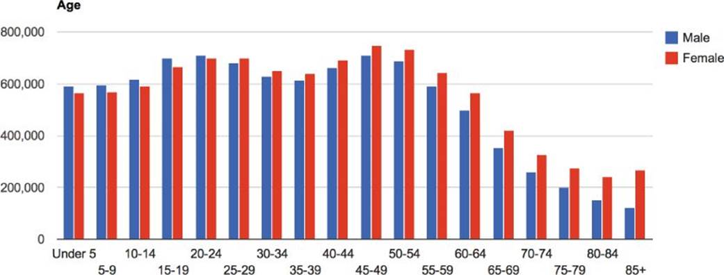
Figure 15.5 This chart shows age by sex information for New York.

You can find this example in the Chapter 15 folder on the companion website. It's named age-chart.html.

Population History Chart

At this point, you've built a number of charts showing various demographic breakdowns. Next, you can take things in a different direction to display population growth over time. However, to access this data you're going to need a different API: the Total Population and Components of Change API you can read about at

1. http://www.census.gov/data/developers/data-sets/population-estimates-and-projections.html

The workflow for this API is largely the same:

1. Create the API call for the data you need.

2. Request that data with Ajax and reformat.

3. Display the data in a Google Chart.

Fortunately (or unfortunately), the data set for this API is significantly smaller than that of the Decennial Census Data, as you can see here: http://api.census.gov/data/2013/pep/natstprc/variables.html. That makes it much easier to build the API call. For example, to grab population change data for New York, you can call:

1. http://api.census.gov/data/2013/pep/natstprc?get=POP,DATE&for=state:36&key=your_api_key

You can use the same API key you used for decennial data, which returns the following:

[["POP","DATE","state"],

["19378102","1","36"],

["19378105","2","36"],

["19398228","3","36"],

["19502728","4","36"],

["19576125","5","36"],

["19651127","6","36"]]

Each row represents another year of population data, from July 1, 2008 (DATE:1) through July 1, 2013 (DATE:6). Next, access this data from your JS and build a chart:

$.ajax({

url: "http://api.census.gov/data/2013/pep/natstprc",

data: {

get: "POP,DATE",

for: "state:36",

key: "[your API key]"

success: function(data) {

var processed = [

["Year", "Population"]

];

for ( i in data ) {

if ( i == 0 ) continue;

processed[i] = [ ∼∼data[i][1] + 2007, ∼∼data[i][0] ];

}

var chartData = google.visualization.arrayToDataTable(processed);

var options = {

title: "Population Growth",

legend: "none"

};

var chart = new google.visualization.LineChart(

document.getElementById("population-chart")

);

chart.draw(chartData, options);

}

});

This script loops through the data the API returns, creating a year string from the DATE values and inserting the population count. It then passes the processed data into Google Charts to render the line chart in Figure 15.6.

c15fig006

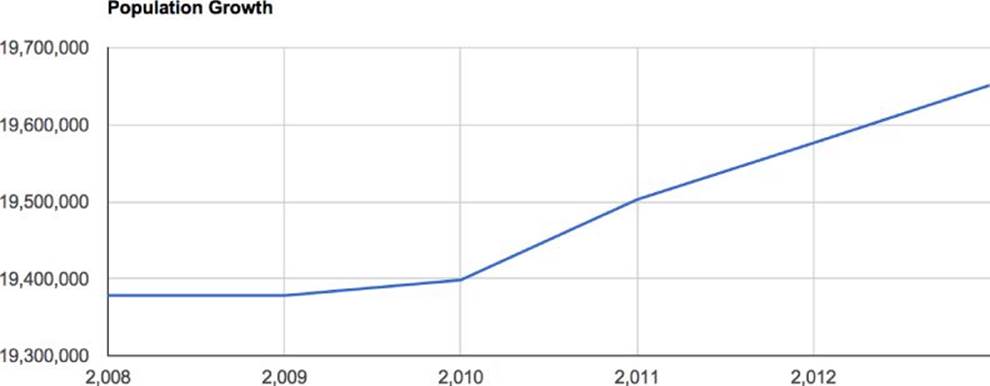
Figure 15.6 This chart shows population growth in New York 2008–2013.

You can find this example in the Chapter 15 folder on the companion website. It's named population-chart.html.

Creating the Dashboard

Now that you've rendered charts for a variety of data sets, you can combine them in a dashboard. For now, you still hardcode the dashboard for New York's data, but it makes an excellent jumping off point for the interactive app.

You can find this example in the Chapter 15 folder on the companion website. It's named responsive-dashboard.html.

Basic Markup and Styling

First, combine the wrappers for each chart in some basic markup:

<h1>

Census Data - New York

</h1>

<h2>

Population

</h2>

</section>

<h2>

Demographics

</h2>

</section>

<h2>

Housing

</h2>

</section>

</div>

Next, apply some basic CSS:

body {

font-family: "Gill Sans", "Gill Sans MT", Calibri, sans-serif;

}

h1, h2 {

font-weight: normal;

}

h2 {

padding: .5em 1em;

background: #DDD;

}

.census {

position: relative;

overflow: hidden;

}

/* charts */

section {

overflow: hidden;

}

.chart {

height: 350px;

}

.demographics .chart, .housing .chart {

width: 50%;

float: left;

}

That renders the charts in the dashboard shown in Figure 15.7.

c15fig007

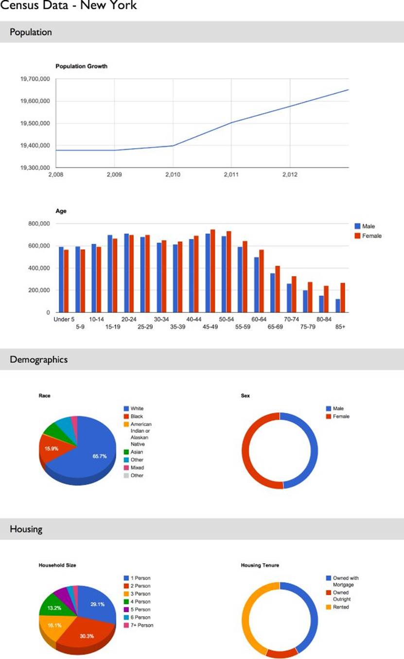
Figure 15.7 At this point the script renders the initial dashboard.

You can find this stylesheet in the Chapter 15 folder on the companion website. It's named css/census-charts.css.

Responsive Layer

So far, the dashboard is looking decent on medium-sized devices. Next, you should add a responsive layer to maximize the screen real estate for both tiny mobile devices and large desktop monitors. To do so, add some simple media queries to the CSS:

@media all and (min-width: 700px) and (max-width: 1000px) {

.demographics .chart, .housing .chart {

width: 50%;

float: left;

}

@media all and (min-width: 1001px) {

.population:not(.single) {

width: 66.6666%;

float: left;

}

.demographics {

width: 33.3333%;

float: right;

}

.housing {

clear: both;

}

.housing .chart {

width: 50%;

float: left;

}

Here, the styles for .demographics .chart, .housing .chart {} have been moved into a block that displays only on windows between 700 and 1000 pixels. That ensures that smaller windows, such as those on phones, don't get the columned layout for these charts and instead display each line by line.

Additionally, some styles have been added for windows larger than 1000px wide. These new rules reposition the demographics column next to the population data, with the two housing charts floated underneath. That gives a much more integrated dashboard feel for larger monitors, which you can see in Figure 15.8.

c15fig008

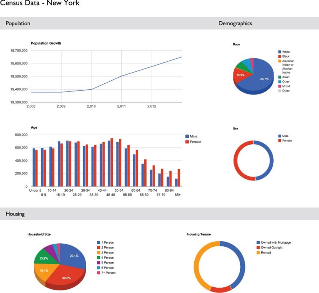
Figure 15.8 This screenshot shows the larger layout for the dashboard.

You can find this stylesheet in the Chapter 15 folder on the companion website. It's named css/census-charts.css.

Connecting Components with Backbone

Now that you've built all the necessary components, it's time to integrate them into an application. To provide some structure for this app, you build it on top of Backbone. The Backbone implementation is fairly lightweight because the app is relatively simple.

The script has to handle three tasks:

1. Render charts of national data for the app's home screen.

2. Create a drop-down menu of states.

3. Use that drop-down menu to render the charts for a given state using its FIPS code.

You can find this example in the Chapter 15 folder on the companion website. It's named css/census-charts.html.

Establishing Models and Collections

To get started, you create some models and collections to work with. First, add a model for general app settings and variables:

var Census = Backbone.Model.extend({

defaults: {

loc: "00",

loc_str: "United States"

validate: function( options ) {

if ( ! options.api_key ) {

return "You must enter your API key from www.census.gov/developers/";

}

initialize: function() {

this.on("invalid", function(e, error) {

console.log(error);

});

}

});

As you can see, the script first defines some defaults for the location FIPS code (loc) and the associated display name (loc_str). Next, it creates a validation function that checks for an API key when the model initializes. The idea is to pass in your API key when you instantiate the model:

var census = new Census({

api_key: "[your API key]"

});

Next, add a model for state data, such as the state name and FIPS code:

var States = Backbone.Collection.extend();

var states = new States([

{ name: "United States", fips: "00" },

{ name: "Alabama", fips: "01" },

{ name: "Alaska", fips: "02" },

{ name: "Arizona", fips: "04" },

{ name: "Arkansas", fips: "05" },

{ name: "California", fips: "06" },

{ name: "Colorado", fips: "08" },

{ name: "Connecticut", fips: "09" },

{ name: "Delaware", fips: "10" },

{ name: "District of Columbia", fips: "11" },

{ name: "Florida", fips: "12" },

{ name: "Georgia", fips: "13" },

{ name: "Hawaii", fips: "15" },

{ name: "Idaho", fips: "16" },

{ name: "Illinois", fips: "17" },

{ name: "Indiana", fips: "18" },

{ name: "Iowa", fips: "19" },

{ name: "Kansas", fips: "20" },

{ name: "Kentucky", fips: "21" },

{ name: "Louisiana", fips: "22" },

{ name: "Maine", fips: "23" },

{ name: "Maryland", fips: "24" },

{ name: "Massachusetts", fips: "25" },

{ name: "Michigan", fips: "26" },

{ name: "Minnesota", fips: "27" },

{ name: "Mississippi", fips: "28" },

{ name: "Missouri", fips: "29" },

{ name: "Montana", fips: "30" },

{ name: "Nebraska", fips: "31" },

{ name: "Nevada", fips: "32" },

{ name: "New Hampshire", fips: "33" },

{ name: "New Jersey", fips: "34" },

{ name: "New Mexico", fips: "35" },

{ name: "New York", fips: "36" },

{ name: "North Carolina", fips: "37" },

{ name: "North Dakota", fips: "38" },

{ name: "Ohio", fips: "39" },

{ name: "Oklahoma", fips: "40" },

{ name: "Oregon", fips: "41" },

{ name: "Pennsylvania", fips: "42" },

{ name: "Rhode Island", fips: "44" },

{ name: "South Carolina", fips: "45" },

{ name: "South Dakota", fips: "46" },

{ name: "Tennessee", fips: "47" },

{ name: "Texas", fips: "48" },

{ name: "Utah", fips: "49" },

{ name: "Vermont", fips: "50" },

{ name: "Virginia", fips: "51" },

{ name: "Washington", fips: "53" },

{ name: "West Virginia", fips: "54" },

{ name: "Wisconsin", fips: "55" },

{ name: "Wyoming", fips: "56" }

]);

You'll use this model for a variety of purposes, such as cross-referencing FIPS codes and display names.

You can find the JavaScript for this example in the Chapter 15 folder on the companion website. It's named js/census-charts.js.

Converting the Chart Markup to a JavaScript Template

Next, convert the chart markup to a JavaScript template:

<h1>

Census Data - <%= loc_str %>

</h1>

<h2>

Population

</h2>

</section>

<h2>

Demographics

</h2>

</section>

<h2>

Housing

</h2>

</section>

</script>

As you can see, the template is mostly static at this point, except for adding the location string to the <h1>. That's because Google Charts handles the majority of the visual heavy lifting.

Next, create the initial view for this template in Backbone:

var CensusView = Backbone.View.extend({

el: ".charts",

initialize: function() {

this.model.on("change", this.render, this);

google.load("visualization", "1", {packages:["corechart"]});

google.setOnLoadCallback($.proxy(this.render, this));

// render the new charts based on this location

render: function() {

// render the main template

var compiled = this.template( this.model.toJSON() );

this.$el.html(compiled);

renderCharts();

return this;

}

});

var censusView = new CensusView({

model: census,

collection: states

});

There are a few things going on in this script:

· The view first binds itself to the .charts node in the Document Object Model (DOM) and builds an Underscore template from the markup you created earlier.

· When the view initializes, it establishes a change handler to rerender the charts whenever the model changes. This will come in handy when you want to switch between states.

· The Google Chart loaders have been moved into this view because they only affect rendering.

· The render function regenerates the markup from the template, inserts it into the DOM, and then calls the renderCharts() script you wrote earlier. Eventually, you'll move the calls from that script into your Backbone implementation, but leave it out for now.

· When instantiating the view, the script passes in both the census model as well as the states collection you created earlier.

Creating the State Drop-down Menu

Next, in order to make the app dynamic, you're going to need form controls, in particular a drop-down menu for states. First create a template for the drop-down menu:

<% _.each(states, function(state) {

%> <option value="<%- state.fips %>"><%- state.name %></option>

<% }); %>

</select>

</script>

This template accepts an array of state name–FIPS pairs and displays them as markup. Next, add the functionality for the drop-down menu to the view:

var CensusView = Backbone.View.extend({

el: ".charts",

initialize: function() {

this.model.on("change", this.render, this);

this.buildDropdown();

google.load("visualization", "1", {packages:["corechart"]});

google.setOnLoadCallback($.proxy(this.render, this));

// builds the state dropdown with change listener

buildDropdown: function() {

// compile the state dropdown template

var tpl = _.template( $(".state-dropdown-tpl").text() ),

compiled = tpl({

states: this.collection.toJSON()

});

// append to the DOM

var $dropdown = $(compiled).appendTo( this.$el.parent() );

$dropdown.on("change", $.proxy(function(e) {

this.model.set({

loc: $dropdown.val(),

loc_str: $dropdown.find("option:selected").text()

});

}, this));

// render the new charts based on this location

render: function() {

// render the main template

var compiled = this.template( this.model.toJSON() );

this.$el.html(compiled);

renderCharts();

return this;

});

In this code, the buildDropdown() function first compiles the drop-down menu template using the hard-coded States collection. Next, it binds a change listener to the drop-down menu, which modifies the Census model with an updated state name and FIPS code. That automatically rerenders the view because it in turn triggers the change handler on the model.

Finally, add some simple styling for the drop-down menu in your CSS:

.state-select {

position: absolute;

top: .8em;

right: 0;

font-size: 2em;

}

As you can see in Figure 15.9, the drop-down menu is now rendering at the top of your charts. However, it still isn't changing the charts for each state because you haven't added those hooks to your renderChart() function.

Figure 15.9 The state drop-down menu.

Rendering State Changes

The next step is integrating the code from renderCharts() into the Backbone application. You can add them one at a time to the view, starting with the population growth chart.

Population Growth Chart

First, create a function in the view to render the population growth chart:

var CensusView = Backbone.View.extend({

el: ".charts",

...

render: function() {

// render the main template

var compiled = this.template( this.model.toJSON() );

this.$el.html(compiled);

// create the charts from this markup

this.renderPopulation();

return this;

renderPopulation: function() {

$.ajax({

url: "http://api.census.gov/data/2013/pep/natstprc",

data: {

get: "POP,DATE",

for: this.model.get("loc_query"),

key: this.model.get("api_key")

success: function(data) {

var processed = [

["Year", "Population"]

];

for ( i in data ) {

if ( i == 0 ) continue;

processed[i] = [ ∼∼data[i][1] + 2007, ∼∼data[i][0] ];

}

var chartData = google.visualization.arrayToDataTable(processed);

var options = {

title: "Population Growth",

legend: "none"

};

var chart = new google.visualization.LineChart(

document.getElementById("population-chart")

);

chart.draw(chartData, options);

}

});

}

});

Here the script is largely the same as before, with one key difference: You've added dynamic references to the model's api_key and loc_query values. You should already have the api_key from when you instantiated the census model, but you still need to do a bit of work to generate the loc_query string, which helps drive the APIs. Add a bit of code to the model that creates this loc_query whenever the loc value is modified:

var Census = Backbone.Model.extend({

defaults: {

loc: "00",

loc_str: "United States"

validate: function( options ) {

if ( ! options.api_key ) {

return "You must enter your API key from www.census.gov/developers/";

}

// creates new location string for API

buildLocQuery: function() {

var loc = this.get("loc");

if ( loc === "00" ) {

this.set("loc_query", "us");

}

else {

this.set("loc_query", "state:" + loc);

}

initialize: function() {

this.on("invalid", function(e, error) {

console.log(error);

});

this.on("change:loc", this.buildLocQuery, this);

this.buildLocQuery();

}

});

This code adds a buildLocQuery() function to the Census model, which creates a query string from this data, switching between national and state-specific data. This function is called both when the model initializes and also any time the loc value in the model changes. That ensures that loc_query stays fresh.

Now if you load the script in your browser, you should see the first bit of dynamic behavior. It's only rendering the population growth chart so far, but that chart is changing dynamically as you switch states in the drop-down menu.

National Versus State Data

Next, you can follow the patterns in the population growth chart to establish the other charts. However, pulling national data for these other charts is a bit more complicated because the Census API doesn't aggregate much data nationally. For now, just disable these in the national view by making some changes to the template:

<h1>

Census Data - <%= loc_str %>

</h1>

<h2>

Population

</h2>

if ( loc !== "00" ) {

}

</section>

if ( loc !== "00" ) {

<h2>

Demographics

</h2>

</section>

<h2>

Housing

</h2>

</section>

}

</script>

As you can see, a few hooks have been added to remove the markup for certain charts at the national level (whenever loc === "00"). Additionally, as you build the other charts, you can add these hooks to your render function.

Age by Sex Chart

Now add the age by sex chart into your view object:

renderAge: function() {

// get sex by age

// build age request string

function build_age_request_string(offset) {

var out = "";

for ( var i = 0; i < 23; i++ ) {

var this_index = ("0" + (i + offset)).slice(-2);

out += "P01200" + this_index + ",";

}

return out;

}

var age_request_keys = build_age_request_string(3) +

build_age_request_string(27);

age_request_keys = age_request_keys.slice(0,-1);

$.ajax({

url: "http://api.census.gov/data/2010/sf1",

data: {

get: age_request_keys,

for: this.model.get("loc_query"),

key: this.model.get("api_key")

success: function(data) {

var male_data = data[1].slice(0,23),

female_data = data[1].slice(23,46);

// merge the dissimilar age ranges

function combine_vals(arr, start, end) {

var total = 0;

for ( var i = start; i <= end; i++ ) {

total += arr[i];

}

arr[start] = total;

arr.splice( start + 1, end - start);

return arr;

}

function clean_age_range( age_data ) {

// convert all the values to numeric

for ( var i in age_data ) {

age_data[i] = ∼∼age_data[i];

}

// merge values starting with highest (to preserve array keys)

// merge 65-66 && 67-69

age_data = combine_vals( age_data, 17, 18 );

// merge 60-61 & 62-64

age_data = combine_vals( age_data, 15, 16 );

// merge 20, 21 & 22-24

age_data = combine_vals( age_data, 5, 7 );

// merge 15-17 & 18-19

age_data = combine_vals( age_data, 3, 4 );

return age_data;

}

male_data = clean_age_range(male_data);

female_data = clean_age_range(female_data);

var processed = [

["Age", "Male", "Female"]

];

for ( var i = 0, max = male_data.length; i < max; i++ ) {

var row = [];

switch(i) {

case 0:

row[0] = "Under 5";

break;

default:

row[0] = (i * 5) + "-" + (i * 5 + 4);

break;

case max - 1:

row[0] = (i * 5) + "+";

break;

}

row[1] = male_data[i];

row[2] = female_data[i];

processed.push(row);

}

var chartData = google.visualization.arrayToDataTable(processed);

var options = {

title: "Age"

};

var chart = new google.visualization.ColumnChart(

document.getElementById("age-chart")

);

chart.draw(chartData, options);

}

});

Again, the only differences between this script and the one previous are the dynamic references to the model's loc_query and api_key values. Next, add this call to the view's render() function, making sure to disable it at the national level:

render: function() {

// render the main template

var compiled = this.template( this.model.toJSON() );

this.$el.html(compiled);

// create the charts from this markup

this.renderPopulation();

// render the other charts if not the national data

if ( this.model.get("loc") !== "00" ) {

this.renderAge();

}

return this;

Other Charts

As you can see, integrating the chart modules into the Backbone app is pretty straightforward—simply set up the dynamic loc_query and api_key values in the Ajax calls. Rather than walk through each of these individually, take a look at the script all together inListing 15-1.

Listing 15-1

var Census = Backbone.Model.extend({

defaults: {

loc: "00",

loc_str: "United States"

validate: function( options ) {

if ( ! options.api_key ) {

return "You must enter your API key from www.census.gov/developers/";

}

// creates new location string for API

buildLocQuery: function() {

var loc = this.get("loc");

if ( loc === "00" ) {

this.set("loc_query", "us");

}

else {

this.set("loc_query", "state:" + loc);

}

initialize: function() {

this.on("invalid", function(e, error) {

console.log(error);

});

this.on("change:loc", this.buildLocQuery, this);

this.buildLocQuery();

}

});

var States = Backbone.Collection.extend();

var states = new States([

{ name: "United States", fips: "00" },

{ name: "Alabama", fips: "01" },

{ name: "Alaska", fips: "02" },

{ name: "Arizona", fips: "04" },

{ name: "Arkansas", fips: "05" },

{ name: "California", fips: "06" },

{ name: "Colorado", fips: "08" },

{ name: "Connecticut", fips: "09" },

{ name: "Delaware", fips: "10" },

{ name: "District of Columbia", fips: "11" },

{ name: "Florida", fips: "12" },

{ name: "Georgia", fips: "13" },

{ name: "Hawaii", fips: "15" },

{ name: "Idaho", fips: "16" },

{ name: "Illinois", fips: "17" },

{ name: "Indiana", fips: "18" },

{ name: "Iowa", fips: "19" },

{ name: "Kansas", fips: "20" },

{ name: "Kentucky", fips: "21" },

{ name: "Louisiana", fips: "22" },

{ name: "Maine", fips: "23" },

{ name: "Maryland", fips: "24" },

{ name: "Massachusetts", fips: "25" },

{ name: "Michigan", fips: "26" },

{ name: "Minnesota", fips: "27" },

{ name: "Mississippi", fips: "28" },

{ name: "Missouri", fips: "29" },

{ name: "Montana", fips: "30" },

{ name: "Nebraska", fips: "31" },

{ name: "Nevada", fips: "32" },

{ name: "New Hampshire", fips: "33" },

{ name: "New Jersey", fips: "34" },

{ name: "New Mexico", fips: "35" },

{ name: "New York", fips: "36" },

{ name: "North Carolina", fips: "37" },

{ name: "North Dakota", fips: "38" },

{ name: "Ohio", fips: "39" },

{ name: "Oklahoma", fips: "40" },

{ name: "Oregon", fips: "41" },

{ name: "Pennsylvania", fips: "42" },

{ name: "Rhode Island", fips: "44" },

{ name: "South Carolina", fips: "45" },

{ name: "South Dakota", fips: "46" },

{ name: "Tennessee", fips: "47" },

{ name: "Texas", fips: "48" },

{ name: "Utah", fips: "49" },

{ name: "Vermont", fips: "50" },

{ name: "Virginia", fips: "51" },

{ name: "Washington", fips: "53" },

{ name: "West Virginia", fips: "54" },

{ name: "Wisconsin", fips: "55" },

{ name: "Wyoming", fips: "56" }

]);

var CensusView = Backbone.View.extend({

el: ".charts",

initialize: function() {

this.model.on("change", this.render, this);

this.buildDropdown();

google.load("visualization", "1", {packages:["corechart"]});

google.setOnLoadCallback($.proxy(this.render, this));

// builds the state dropdown with change listener

buildDropdown: function() {

// compile the state dropdown template

var tpl = _.template( $(".state-dropdown-tpl").text() ),

compiled = tpl({

states: this.collection.toJSON()

});

// append to the DOM

var $dropdown = $(compiled).appendTo( this.$el.parent() );

$dropdown.on("change", $.proxy(function(e) {

this.model.set({

loc: $dropdown.val(),

loc_str: $dropdown.find("option:selected").text()

});

}, this));

// render the new charts based on this location

render: function() {

// render the main template

var compiled = this.template( this.model.toJSON() );

this.$el.html(compiled);

// create the charts from this markup

this.renderPopulation();

// render the other charts if not the national data

if ( this.model.get("loc") !== "00" ) {

this.renderAge();

this.renderRace();

this.renderSex();

this.renderHousing();

this.renderTenure();

}

return this;

renderPopulation: function() {

$.ajax({

url: "http://api.census.gov/data/2013/pep/natstprc",

data: {

get: "POP,DATE",

for: this.model.get("loc_query"),

key: this.model.get("api_key")

success: function(data) {

var processed = [

["Year", "Population"]

];

for ( i in data ) {

if ( i == 0 ) continue;

processed[i] = [ ∼∼data[i][1] + 2007, ∼∼data[i][0] ];

}

var chartData = google.visualization.arrayToDataTable(processed);

var options = {

title: "Population Growth",

legend: "none"

};

var chart = new google.visualization.LineChart(

document.getElementById("population-chart")

);

chart.draw(chartData, options);

}

});

renderAge: function() {

// get sex by age

// build age request string

function build_age_request_string(offset) {

var out = "";

for ( var i = 0; i < 23; i++ ) {

var this_index = ("0" + (i + offset)).slice(-2);

out += "P01200" + this_index + ",";

}

return out;

}

var age_request_keys = build_age_request_string(3) +

build_age_request_string(27);

age_request_keys = age_request_keys.slice(0,-1);

$.ajax({

url: "http://api.census.gov/data/2010/sf1",

data: {

get: age_request_keys,

for: this.model.get("loc_query"),

key: this.model.get("api_key")

success: function(data) {

var male_data = data[1].slice(0,23),

female_data = data[1].slice(23,46);

// merge the dissimilar age ranges

function combine_vals(arr, start, end) {

var total = 0;

for ( var i = start; i <= end; i++ ) {

total += arr[i];

}

arr[start] = total;

arr.splice( start + 1, end - start);

return arr;

}

function clean_age_range( age_data ) {

// convert all the values to numeric

for ( var i in age_data ) {

age_data[i] = ∼∼age_data[i];

}

// merge values starting with highest (to preserve array keys)

// merge 65-66 && 67-69

age_data = combine_vals( age_data, 17, 18 );

// merge 60-61 & 62-64

age_data = combine_vals( age_data, 15, 16 );

// merge 20, 21 & 22-24

age_data = combine_vals( age_data, 5, 7 );

// merge 15-17 & 18-19

age_data = combine_vals( age_data, 3, 4 );

return age_data;

}

male_data = clean_age_range(male_data);

female_data = clean_age_range(female_data);

var processed = [

["Age", "Male", "Female"]

];

for ( var i = 0, max = male_data.length; i < max; i++ ) {

var row = [];

switch(i) {

case 0:

row[0] = "Under 5";

break;

default:

row[0] = (i * 5) + "-" + (i * 5 + 4);

break;

case max - 1:

row[0] = (i * 5) + "+";

break;

}

row[1] = male_data[i];

row[2] = female_data[i];

processed.push(row);

}

var chartData = google.visualization.arrayToDataTable(processed);

var options = {

title: "Age"

};

var chart = new google.visualization.ColumnChart(

document.getElementById("age-chart")

);

chart.draw(chartData, options);

}

});

renderRace: function() {

// get race data

$.ajax({

url: "http://api.census.gov/data/2010/sf1",

data: {

get: "P0080003,P0080004,P0080005,P0080006,P0080007,P0080008,P0080009",

for: this.model.get("loc_query"),

key: this.model.get("api_key")

success: function(data) {

var races = [

"White",

"Black",

"American Indian or Alaskan Native",

"Asian",

"Native Hawaiian or Pacific Islander",

"Other",

"Mixed"

processed = [

["Race", "Population"]

];

// lose the last value (state ID)

data[1].pop();

for ( i in data[1] ) {

processed.push([

races[i],

∼∼data[1][i]

]);

}

var chartData = google.visualization.arrayToDataTable(processed);

var options = {

title: "Race",

is3D: true

};

var chart = new google.visualization.PieChart(

document.getElementById("race-chart")

);

chart.draw(chartData, options);

}

});

renderSex: function() {

// get basic sex data

$.ajax({

url: "http://api.census.gov/data/2010/sf1",

data: {

get: "P0120002,P0120026",

for: this.model.get("loc_query"),

key: this.model.get("api_key")

success: function(data) {

var processed = [

["Sex", "Population"],

["Male", ∼∼data[1][0]],

["Female", ∼∼data[1][1]]

];

var chartData = google.visualization.arrayToDataTable(processed);

var options = {

title: "Sex",

pieHole: 0.8,

pieSliceText: "none"

};

var chart = new google.visualization.PieChart(

document.getElementById("sex-chart")

);

chart.draw(chartData, options);

}

});

renderHousing: function() {

// get household size

$.ajax({

url: "http://api.census.gov/data/2010/sf1",

data: {

get: "H0130002,H0130003,H0130004,H0130005,H0130006,H0130007,H0130008",

for: this.model.get("loc_query"),

key: this.model.get("api_key")

success: function(data) {

var processed = [

["Household Size", "Households"]

];

// lose the last value (state ID)

data[1].pop();

for ( i in data[1] ) {

processed.push([

(∼∼i+1) + ( i == 6 ? "+" : "" ) + " Person",

∼∼data[1][i]

]);

}

var chartData = google.visualization.arrayToDataTable(processed);

var options = {

title: "Household Size",

is3D: true

};

var chart = new google.visualization.PieChart(

document.getElementById("household-chart")

);

chart.draw(chartData, options);

}

});

renderTenure: function() {

// get housing tenure

$.ajax({

url: "http://api.census.gov/data/2010/sf1",

data: {

get: "H0110002,H0110003,H0110004",

for: this.model.get("loc_query"),

key: this.model.get("api_key")

success: function(data) {

var processed = [

["Tenure", "Housing Units"],

["Owned with Mortgage", ∼∼data[1][0]],

["Owned Outright", ∼∼data[1][1]],

["Rented", ∼∼data[1][2]]

];

var chartData = google.visualization.arrayToDataTable(processed);

var options = {

title: "Housing Tenure",

pieHole: 0.8,

pieSliceText: "none"

};

var chart = new google.visualization.PieChart(

document.getElementById("tenure-chart")

);

chart.draw(chartData, options);

}

});

}

});

var census = new Census({

api_key: "ddda45df6ccb8e1e722aca5f142d7db2a032c330"

});

var censusView = new CensusView({

model: census,

collection: states

});

Here's a recap of what happens:

1. The script creates a Census model to store settings and global variables. This model validates against the api_key and also creates a dynamic loc_query string that adjusts to match the loc value.

2. It then builds a States collection with state names and FIPS codes.

3. The view initializes, binding a change listener to rerender the templates for any change to the model, building the drop-down menu, and loading the Google Charts API.

4. In the render() function, the script recompiles the template and also makes calls to render the individual charts, depending on whether it is at the national level.

Next Steps

Now the script is dynamically rendering charts for various states. But that's really just the bare bones for this application, and there are a number of additional features you can add to the code.

Rerendering on Resize

For instance, you may have noticed that Google doesn't refresh the charts as you resize the window. That's mostly fine, but it can cause some visual issues with the responsive layout. Fortunately it's easy to add a handler to redraw the charts on resize. Simply add the following to the view's initialize() function:

// redraw charts on window resize

var debouncedRender = _.debounce($.proxy(this.render, this), 1000);

$(window).resize(debouncedRender);

While you could have just applied the render() function directly in the resize() callback, it's important to use the debounced approach here. The script leverages Underscore's debounce() utility function to prevent the render() function from firing repeatedly as the user resizes her window. Instead, it fires the resize only after a full second of resizing.

TIP The debounced approach is always useful for window.resize() handlers but is especially so when calling a resource-heavy render such as our Google Charts implementation.

Other Improvements

Additionally, there are a variety of improvements you can add to this script:

· Aggregate the state data to show all the charts at the national level.

· Cache previously visited states in localStorage to avoid unnecessary API calls.

· Enable routing and history using either hashchange or pushState and Backbone's History API.

Summary

In this chapter, you created an interactive dashboard of U.S. Census data. You learned how to work through the headaches of the Census API in order to access a wealth of demographic data. You then massaged this data and displayed it in Google Charts using a responsive layout for the dashboard.

Next you integrated these components into a Backbone app, which dynamically updates the charts based on user input. Finally, you explored some new directions to take the script.

In the next chapter, you follow another practical charting example, this time leveraging D3 to create another set of interactive visualizations.