How Linux Works: What Every Superuser Should Know (2015)

Chapter 9. Understanding your Network and its Configuration

Networking is the practice of connecting computers and sending data between them. That sounds simple enough, but to understand how it works, you need to ask two fundamental questions:

§ How does the computer sending the data know where to send its data?

§ When the destination computer receives the data, how does it know what it just received?

A computer answers these questions by using a series of components, with each one responsible for a certain aspect of sending, receiving, and identifying data. The components are arranged in groups that form network layers, which stack on top of each other in order to form a complete system. The Linux kernel handles networking in a similar way to the SCSI subsystem described in Chapter 3.

Because each layer tends to be independent, it’s possible to build networks with many different combinations of components. This is where network configuration can become very complicated. For this reason, we’ll begin this chapter by looking at the layers in very simple networks. You’ll learn how to view your own network settings, and when you understand the basic workings of each layer, you’ll be ready to learn how to configure those layers by yourself. Finally, you’ll move on to more advanced topics like building your own networks and configuring firewalls. (Skip over that material if your eyes start to glaze over; you can always come back.)

9.1 Network Basics

Before getting into the theory of network layers, take a look at the simple network shown in Figure 9-1.

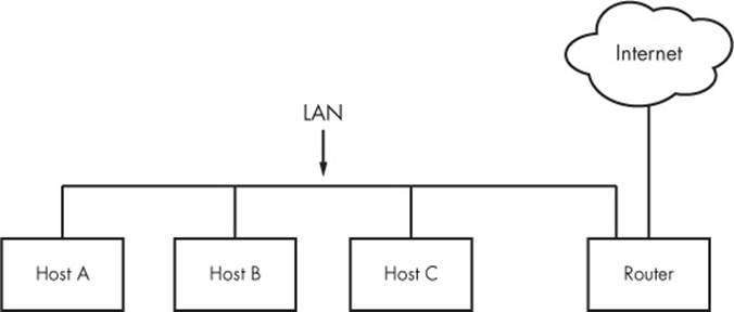
Figure 9-1. A typical local area network with a router that provides Internet access

This type of network is ubiquitous; most home and small office networks are configured this way. Each machine connected to the network is called a host. The hosts are connected to a router, which is a host that can move data from one network to another. These machines (here, Hosts A, B, and C) and the router form a local area network (LAN). The connections on the LAN can be wired or wireless.

The router is also connected to the Internet—the cloud in the figure. Because the router is connected to both the LAN and the Internet, all machines on the LAN also have access to the Internet through the router. One of the goals of this chapter is to see how the router provides this access.

Your initial point of view will be from a Linux-based machine such as Host A on the LAN in Figure 9-1.

9.1.1 Packets

A computer transmits data over a network in small chunks called packets, which consist of two parts: a header and a payload. The header contains identifying information such as the origin/destination hosts and basic protocol. The payload, on the other hand, is the actual application data that the computer wants to send (for example, HTML or image data).

Packets allow a host to communicate with others “simultaneously,” because hosts can send, receive, and process packets in any order, regardless of where they came from or where they’re going. Breaking messages into smaller units also makes it easier to detect and compensate for errors in transmission.

For the most part, you don’t have to worry about translating between packets and the data that your application uses, because the operating system has facilities that do this for you. However, it is helpful to know the role of packets in the network layers that you’re about to see.

9.2 Network Layers

A fully functioning network includes a full set of network layers called a network stack. Any functional network has a stack. The typical Internet stack, from the top to bottom layer, looks like this:

§ Application layer. Contains the “language” that applications and servers use to communicate; usually a high-level protocol of some sort. Common application layer protocols include Hypertext Transfer Protocol (HTTP, used for the Web), Secure Socket Layer (SSL), and File Transfer Protocol (FTP). Application layer protocols can often be combined. For example, SSL is commonly used in conjunction with HTTP.

§ Transport layer. Defines the data transmission characteristics of the application layer. This layer includes data integrity checking, source and destination ports, and specifications for breaking application data into packets (if the application layer has not already done so). Transmission Control Protocol (TCP) and User Datagram Protocol (UDP) are the most common transport layer protocols. The transport layer is also sometimes called the protocol layer.

§ Network or Internet layer. Defines how to move packets from a source host to a destination host. The particular packet transit rule set for the Internet is known as Internet Protocol (IP). Because we’ll only talk about Internet networks in this book, we’ll really only be talking about the Internet layer. However, because network layers are meant to be hardware independent, you can simultaneously configure several independent network layers (such as IP, IPv6, IPX, and AppleTalk) on a single host.

§ Physical layer. Defines how to send raw data across a physical medium, such as Ethernet or a modem. This is sometimes called the link layer or host-to-network layer.

It’s important to understand the structure of a network stack because your data must travel through these layers at least twice before it reaches a program at its destination. For example, if you’re sending data from Host A to Host B, as shown in Figure 9-1, your bytes leave the application layer on Host A and travel through the transport and network layers on Host A; then they go down to the physical medium, across the medium, and up again through the various lower levels to the application layer on Host B in much the same way. If you’re sending something to a host on the Internet through the router, it will go through some (but usually not all) of the layers on the router and anything else in between.

The layers sometimes bleed into each other in strange ways because it can be inefficient to process all of them in order. For example, devices that historically dealt with only the physical layer now sometimes look at the transport and Internet layer data to filter and route data quickly. (Don’t worry about this when you’re learning the basics.)

We’ll begin by looking at how your Linux machine connects to the network in order to answer the where question at the beginning of the chapter. This is the lower part of the stack—the physical and network layers. Later, we’ll look at the upper two layers that answer the what question.

NOTE

You might have heard of another set of layers known as the Open Systems Interconnection (OSI) Reference Model. This is a seven-layer network model often used in teaching and designing networks, but we won’t cover the OSI model because you’ll be working directly with the four layers described here. To learn a lot more about layers (and networks in general), see Andrew S. Tanenbaum and David J. Wetherall’s Computer Networks, 5th edition (Prentice Hall, 2010).

9.3 The Internet Layer

Rather than start at the very bottom of the network stack with the physical layer, we’ll start at the network layer because it can be easier to understand. The Internet as we currently know it is based on the Internet Protocol, version 4 (IPv4), though version 6 (IPv6) is gaining adoption. One of the most important aspects of the Internet layer is that it’s meant to be a software network that places no particular requirements on hardware or operating systems. The idea is that you can send and receive Internet packets over any kind of hardware, using any operating system.

The Internet’s topology is decentralized; it’s made up of smaller networks called subnets. The idea is that all subnets are interconnected in some way. For example, in Figure 9-1, the LAN is normally a single subnet.

A host can be attached to more than one subnet. As you saw in 9.1 Network Basics, that kind of host is called a router if it can transmit data from one subnet to another (another term for router is gateway). Figure 9-2 refines Figure 9-1 by identifying the LAN as a subnet, as well as Internet addresses for each host and the router. The router in the figure has two addresses, the local subnet 10.23.2.1 and the link to the Internet (but this Internet link’s address is not important right now so it’s just marked “Uplink Address”). We’ll look first at the addresses and then the subnet notation.

Each Internet host has at least one numeric IP address in the form of a.b.c.d, such as 10.23.2.37. An address in this notation is called a dotted-quad sequence. If a host is connected to multiple subnets, it has at least one IP address per subnet. Each host’s IP address should be unique across the entire Internet, but as you’ll see later, private networks and NAT can make this a little confusing.

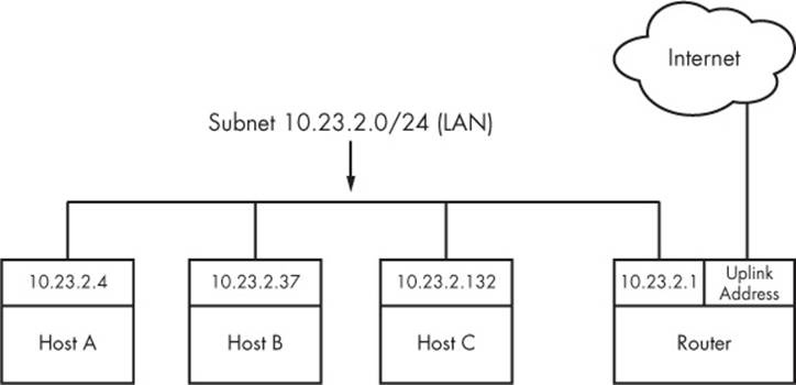
Figure 9-2. Network with IP addresses

NOTE

Technically, an IP address consists of 4 bytes (or 32 bits), abcd. Bytes a and d are numbers from 1 to 254, and b and c are numbers from 0 to 255. A computer processes IP addresses as raw bytes. However, it’s much easier for a human to read and write a dotted-quad address, such as 10.23.2.37, instead of something ugly like the hexadecimal 0x0A170225.

IP addresses are like postal addresses in some ways. To communicate with another host, your machine must know that other host’s IP address.

Let’s take a look at the address on your machine.

9.3.1 Viewing Your Computer’s IP Addresses

One host can have many IP addresses. To see the addresses that are active on your Linux machine, run

$ ifconfig

There will probably be a lot of output, but it should include something like this:

eth0 Link encap:Ethernet HWaddr 10:78:d2:eb:76:97

inet addr:10.23.2.4 Bcast:10.23.2.255 Mask:255.255.255.0

inet6 addr: fe80::1278:d2ff:feeb:7697/64 Scope:Link

UP BROADCAST RUNNING MULTICAST MTU:1500 Metric:1

RX packets:85076006 errors:0 dropped:0 overruns:0 frame:0

TX packets:68347795 errors:0 dropped:0 overruns:0 carrier:0

collisions:0 txqueuelen:1000

RX bytes:86427623613 (86.4 GB) TX bytes:23437688605 (23.4 GB)

Interrupt:20 Memory:fe500000-fe520000

The ifconfig command’s output includes many details from both the Internet layer and the physical layer. (Sometimes it doesn’t even include an Internet address at all!) We’ll discuss the output in more detail later, but for now, concentrate on the second line, which reports that the host isconfigured to have an IPv4 address (inet addr) of 10.23.2.4. On the same line, a Mask is reported as being 255.255.255.0. This is a subnet mask, which defines the subnet that an IP address belongs to. Let’s see how that works.

NOTE

The ifconfig command, as well some of the others you’ll see later in this chapter (such as route and arp), has been technically supplanted with the newer ip command. The ip command can do more than the old commands, and it is preferable when writing scripts. However, most people still use the old commands when manually working with the network, and these commands can also be used on other versions of Unix. For this reason, we’ll use the old-style commands.

9.3.2 Subnets

A subnet is a connected group of hosts with IP addresses in some sort of order. Usually, the hosts are on the same physical network, as shown in Figure 9-2. For example, the hosts between 10.23.2.1 and 10.23.2.254 could comprise a subnet, as could all hosts between 10.23.1.1 and 10.23.255.254.

You define a subnet with two pieces: a network prefix and a subnet mask (such as the one in the output of ifconfig in the previous section). Let’s say you want to create a subnet containing the IP addresses between 10.23.2.1 and 10.23.2.254. The network prefix is the part that is common to all addresses in the subnet; in this example, it’s 10.23.2.0, and the subnet mask is 255.255.255.0. Let’s see why those are the right numbers.

It’s not immediately clear how the prefix and mask work together to give you all possible IP addresses on a subnet. Looking at the numbers in binary form helps clear it up. The mask marks the bit locations in an IP address that are common to the subnet. For example, here are the binary forms of 10.23.2.0 and 255.255.255.0:

10.23.2.0: 00001010 00010111 00000010 00000000

255.255.255.0: 11111111 11111111 11111111 00000000

Now, let’s use boldface to mark the bit locations in 10.23.2.0 that are 1s in 255.255.255.0:

10.23.2.0: 00001010 00010111 00000010 00000000

Look at the bits that are not in bold. You can set any number of these bits to 1 to get a valid IP address in this subnet, with the exception of all 0s or all 1s.

Putting it all together, you can see how a host with an IP address of 10.23.2.1 and a subnet mask of 255.255.255.0 is on the same subnet as any other computers that have IP addresses beginning with 10.23.2. You can denote this entire subnet as 10.23.2.0/255.255.255.0.

9.3.3 Common Subnet Masks and CIDR Notation

If you’re lucky, you’ll only deal with easy subnet masks like 255.255.255.0 or 255.255.0.0, but you may be unfortunate and encounter stuff like 255.255.255.192, where it isn’t quite so simple to determine the set of addresses that belong to the subnet. Furthermore, it’s likely that you’ll also encounter a different form of subnet representation called Classless Inter-Domain Routing (CIDR) notation, where a subnet such as 10.23.2.0/255.255.255.0 is written as 10.23.2.0/24.

To understand what this means, look at the mask in binary form (as in the example you saw in the preceding section). You’ll find that nearly all subnet masks are just a bunch of 1s followed by a bunch of 0s. For example, you just saw that 255.255.255.0 in binary form is 24 1-bits followed by 8 0-bits. The CIDR notation identifies the subnet mask by the number of leading 1s in the subnet mask. Therefore, a combination such as 10.23.2.0/24 includes both the subnet prefix and its subnet mask.

Table 9-1 shows several example subnet masks and their CIDR forms.

Table 9-1. Subnet Masks

NOTE

If you aren’t familiar with conversion between decimal, binary, and hexadecimal formats, you can use a calculator utility such as bc or dc to convert between different radix representations. For example, in bc, you can run the command obase=2; 240 to print the number 240 in binary (base 2) form.

Identifying subnets and their hosts is the first building block to understanding how the Internet works. However, you still need to connect the subnets.

9.4 Routes and the Kernel Routing Table

Connecting Internet subnets is mostly a process of identifying the hosts connected to more than one subnet. Returning to Figure 9-2, think about Host A at IP address 10.23.2.4. This host is connected to a local network of 10.23.2.0/24 and can directly reach hosts on that network. To reach hosts on the rest of the Internet, it must communicate through the router at 10.23.2.1.

How does the Linux kernel distinguish between these two different kinds of destinations? It uses a destination configuration called a routing table to determine its routing behavior. To show the routing table, use the route -n command. Here’s what you might see for a simple host such as 10.23.2.4:

$ route -n

Kernel IP routing table

Destination Gateway Genmask Flags Metric Ref Use Iface

0.0.0.0 10.23.2.1 0.0.0.0 UG 0 0 0 eth0

10.23.2.0 0.0.0.0 255.255.255.0 U 1 0 0 eth0

The last two lines here contain the routing information. The Destination column tells you a network prefix, and the Genmask column is the netmask corresponding to that network. There are two networks defined in this output: 0.0.0.0/0 (which matches every address on the Internet) and 10.23.2.0/24. Each network has a U under its Flags column, indicating that the route is active (“up”).

Where the destinations differ is in the combination of their Gateway and Flags columns. For 0.0.0.0/0, there is a G in the Flags column, meaning that communication for this network must be sent through the gateway in the Gateway column (10.23.2.1, in this case). However, for 10.23.2.0/24, there is no G in Flags, indicating that the network is directly connected in some way. Here, 0.0.0.0 is used as a stand-in under Gateway. Ignore the other columns of output for now.

There’s one tricky detail: Say the host wants to send something to 10.23.2.132, which matches both rules in the routing table, 0.0.0.0/0 and 10.23.2.0/24. How does the kernel know to use the second one? It chooses the longest destination prefix that matches. This is where CIDR network form comes in particularly handy: 10.23.2.0/24 matches, and its prefix is 24 bits long; 0.0.0.0/0 also matches, but its prefix is 0 bits long (that is, it has no prefix), so the rule for 10.23.2.0/24 takes priority.

NOTE

The -n option tells route to show IP addresses instead of showing hosts and networks by name. This is an important option to remember because you’ll be able to use it in other network-related commands such as netstat.

9.4.1 The Default Gateway

An entry for 0.0.0.0/0 in the routing table has special significance because it matches any address on the Internet. This is the default route, and the address configured under the Gateway column (in the route -n output) in the default route is the default gateway. When no other rules match, the default route always does, and the default gateway is where you send messages when there is no other choice. You can configure a host without a default gateway, but it won’t be able to reach hosts outside the destinations in the routing table.

NOTE

On most networks with a netmask of 255.255.255.0, the router is usually at address 1 of the subnet (for example, 10.23.2.1 in 10.23.2.0/24). Because this is simply a convention, there can be exceptions.

9.5 Basic ICMP and DNS Tools

Now it’s time to look at some basic practical utilities to help you interact with hosts. These tools use two protocols of particular interest: Internet Control Message Protocol (ICMP), which can help you root out problems with connectivity and routing, and the Domain Name Service (DNS) system, which maps names to IP addresses so that you don’t have to remember a bunch of numbers.

9.5.1 ping

ping (see http://ftp.arl.mil/~mike/ping.html) is one of the most basic network debugging tools. It sends ICMP echo request packets to a host that ask a recipient host to return the packet to the sender. If the recipient host gets the packet and is configured to reply, it sends an ICMP echo response packet in return.

For example, say that you run ping 10.23.2.1 and get this output:

$ ping 10.23.2.1

PING 10.23.2.1 (10.23.2.1) 56(84) bytes of data.

64 bytes from 10.23.2.1: icmp_req=1 ttl=64 time=1.76 ms

64 bytes from 10.23.2.1: icmp_req=2 ttl=64 time=2.35 ms

64 bytes from 10.23.2.1: icmp_req=4 ttl=64 time=1.69 ms

64 bytes from 10.23.2.1: icmp_req=5 ttl=64 time=1.61 ms

The first line says that you’re sending 56-byte packets (84 bytes, if you include the headers) to 10.23.2.1 (by default, one packet per second), and the remaining lines indicate responses from 10.23.2.1. The most important parts of the output are the sequence number (icmp_req) and the round-trip time (time). The number of bytes returned is the size of the packet sent plus 8. (The content of the packets isn’t important to you.)

A gap in the sequence numbers, such as the one between 2 and 4, usually means there’s some kind of connectivity problem. It’s possible for packets to arrive out of order, and if they do, there’s some kind of problem because ping sends only one packet a second. If a response takes more than a second (1000ms) to arrive, the connection is extremely slow.

The round-trip time is the total elapsed time between the moment that the request packet leaves and moment that the response packet arrives. If there’s no way to reach the destination, the final router to see the packet returns an ICMP “host unreachable” packet to ping.

On a wired LAN, you should expect absolutely no packet loss and very low numbers for the round-trip time. (The preceding example output is from a wireless network.) You should also expect no packet loss from your network to and from your ISP and reasonably steady round-trip times.

NOTE

For security reasons, not all hosts on the Internet respond to ICMP echo request packets, so you might find that you can connect to a website on a host but not get a ping response.

9.5.2 traceroute

The ICMP-based program traceroute will come in handy when you reach the material on routing later in this chapter. Use traceroute host to see the path your packets take to a remote host. (traceroute -n host will disable hostname lookups.)

One of the best things about traceroute is that it reports return trip times at each step in the route, as demonstrated in this output fragment:

4 206.220.243.106 1.163 ms 0.997 ms 1.182 ms

5 4.24.203.65 1.312 ms 1.12 ms 1.463 ms

6 64.159.1.225 1.421 ms 1.37 ms 1.347 ms

7 64.159.1.38 55.642 ms 55.625 ms 55.663 ms

8 209.247.10.230 55.89 ms 55.617 ms 55.964 ms

9 209.244.14.226 55.851 ms 55.726 ms 55.832 ms

10 209.246.29.174 56.419 ms 56.44 ms 56.423 ms

Because this output shows a big latency jump between hops 6 and 7, that part of the route is probably some sort of long-distance link.

The output from traceroute can be inconsistent. For example, the replies may time out at a certain step, only to “reappear” in later steps. The reason is usually that the router at that step refused to return the debugging output that traceroute wants but routers in later steps were happy to return the output. In addition, a router might choose to assign a lower priority to the debugging traffic than it does to normal traffic.

9.5.3 DNS and host

IP addresses are difficult to remember and subject to change, which is why we normally use names such as www.example.com instead. The DNS library on your system normally handles this translation automatically, but sometimes you’ll want to manually translate between a name and an IP address. To find the IP address behind a domain name, use the host command:

$ host www.example.com

www.example.com has address 93.184.216.119

www.example.com has IPv6 address 2606:2800:220:6d:26bf:1447:1097:aa7

Notice how this example has both the IPv4 address 93.184.216.119 and the much larger IPv6 address. This means that this host also has an address on the next-generation version of the Internet.

You can also use host in reverse: Enter an IP address instead of a hostname to try to discover the hostname behind the IP address. But don’t expect this to work reliably. Many hostnames can represent a single IP address, and DNS doesn’t know how to determine which hostname should correspond to an IP address. The domain administrator must manually set up this reverse lookup, and often the administrator does not. (There is a lot more to DNS than the host command. We’ll cover basic client configuration later in 9.12 Resolving Hostnames.)

9.6 The Physical Layer and Ethernet

One of the key things to understand about the Internet is that it’s a software network. Nothing we’ve discussed so far is hardware specific, and indeed, one reason for the Internet’s success is that it works on almost any kind of computer, operating system, and physical network. However, you still have to put a network layer on top of some kind of hardware, and that interface is called the physical layer.

In this book, we’ll look at the most common kind of physical layer: an Ethernet network. The IEEE 802 family of standards documents defines many different kinds of Ethernet networks, from wired to wireless, but they all have a few things in common, in particular, the following:

§ All devices on an Ethernet network have a Media Access Control (MAC) address, sometimes called a hardware address. This address is independent of a host’s IP address, and it is unique to the host’s Ethernet network (but not necessarily a larger software network such as the Internet). A sample MAC address is 10:78:d2:eb:76:97.

§ Devices on an Ethernet network send messages in frames, which are wrappers around the data sent. A frame contains the origin and destination MAC addresses.

Ethernet doesn’t really attempt to go beyond hardware on a single network. For example, if you have two different Ethernet networks with one host attached to both networks (and two different network interface devices), you can’t directly transmit a frame from one Ethernet network to the other unless you set up a special Ethernet bridge. And this is where higher network layers (such as the Internet layer) come in. By convention, each Ethernet network is also usually an Internet subnet. Even though a frame can’t leave one physical network, a router can take the data out of a frame, repackage it, and send it to a host on a different physical network, which is exactly what happens on the Internet.

9.7 Understanding Kernel Network Interfaces

The physical and the Internet layers must be connected in a way that allows the Internet layer to retain its hardware-independent flexibility. The Linux kernel maintains its own division between the two layers and provides communication standards for linking them called a (kernel) network interface. When you configure a network interface, you link the IP address settings from the Internet side with the hardware identification on the physical device side. Network interfaces have names that usually indicate the kind of hardware underneath, such as eth0 (the first Ethernet card in the computer) and wlan0 (a wireless interface).

In 9.3.1 Viewing Your Computer’s IP Addresses, you learned the most important command for viewing or manually configuring the network interface settings: ifconfig. Recall this output:

eth0 Link encap:Ethernet HWaddr 10:78:d2:eb:76:97

inet addr:10.23.2.4 Bcast:10.23.2.255 Mask:255.255.255.0

inet6 addr: fe80::1278:d2ff:feeb:7697/64 Scope:Link

UP BROADCAST RUNNING MULTICAST MTU:1500 Metric:1

RX packets:85076006 errors:0 dropped:0 overruns:0 frame:0

TX packets:68347795 errors:0 dropped:0 overruns:0 carrier:0

collisions:0 txqueuelen:1000

RX bytes:86427623613 (86.4 GB) TX bytes:23437688605 (23.4 GB)

Interrupt:20 Memory:fe500000-fe520000

For each network interface, the left side of the output shows the interface name, and the right side contains settings and statistics for the interface. In addition to the Internet layer pieces that we’ve already covered, you also see the MAC address on the physical layer (HWaddr). The lines containing UP and RUNNING tell you that the interface is working.

Although ifconfig shows some hardware information (in this case, even some low-level device settings such as the interrupt and memory used), it’s designed primarily for viewing and configuring the software layers attached to the interfaces. To dig deeper into the hardware and physical layer behind a network interface, use something like the ethtool command to display or change the settings on Ethernet cards. (We’ll look briefly at wireless networks in 9.23 Wireless Ethernet.)

9.8 Introduction to Network Interface Configuration

You’ve now seen all of the basic elements that go into the lower levels of a network stack: the physical layer, the network (Internet) layer, and the Linux kernel’s network interfaces. In order to combine these pieces to connect a Linux machine to the Internet, you or a piece of software must do the following:

1. Connect the network hardware and ensure that the kernel has a driver for it. If the driver is present, ifconfig -a displays a kernel network interface corresponding to the hardware.

2. Perform any additional physical layer setup, such as choosing a network name or password.

3. Bind an IP address and netmask to the kernel network interface so that the kernel’s device drivers (physical layer) and Internet subsystems (Internet layer) can talk to each other.

4. Add any additional necessary routes, including the default gateway.

When all machines were big stationary boxes wired together, this was relatively straightforward: The kernel did step 1, you didn’t need step 2, and you’d do step 3 with the ifconfig command and step 4 with the route command.

To manually set the IP address and netmask for a kernel network interface, you’d do this:

# ifconfig interface address netmask mask

Here, interface is the name of the interface, such as eth0. When the interface was up, you’d be ready to add routes, which was typically just a matter of setting the default gateway, like this:

# route add default gw gw-address

The gw-address parameter is the IP address of your default gateway; it must be an address in a locally connected subnet defined by the address and mask settings of one of your network interfaces.

9.8.1 Manually Adding and Deleting Routes

To remove a default gateway, run

# route del -net default

You can easily override the default gateway with other routes. For example, say your machine is on subnet 10.23.2.0/24, you want to reach a subnet at 192.168.45.0/24, and you know that 10.23.2.44 can act as a router for that subnet. Run this command to send traffic bound for 192.168.45.0 to that router:

# route add -net 192.168.45.0/24 gw 10.23.2.44

You don’t need to specify the router in order to delete a route:

# route del -net 192.168.45.0/24

Now, before you go crazy with routes, you should know that messing with routes is often more complicated than it appears. For this particular example, you also have to make sure that the routing for all hosts on 192.163.45.0/24 can lead back to 10.23.2.0/24, or the first route you add is basically useless.

Normally, you should keep things as simple as possible for your clients, setting up networks so that their hosts need only a default route. If you need multiple subnets and the ability to route between them, it’s usually best to configure the routers acting as the default gateways to do all of the work of routing between different local subnets. (You’ll see an example in 9.17 Configuring Linux as a Router.)

9.9 Boot-Activated Network Configuration

We’ve discussed ways to manually configure a network, and the traditional way to ensure the correctness of a machine’s network configuration was to have init run a script to run the manual configuration at boot time. This boils down to running tools like ifconfig and route somewhere in the chain of boot events. Many servers still do it this way.

There have been many attempts in Linux to standardize configuration files for boot-time networking. The tools ifup and ifdown do so—for example, a boot script can (in theory) run ifup eth0 to run the correct ifconfig and route commands for the eth0 interface. Unfortunately, different distributions have completely different implementations of ifup and ifdown, and as a result, their configuration files are also completely different. Ubuntu, for example, uses the ifupdown suite with configuration files in /etc/network, and Fedora uses its own set of scripts with configuration in /etc/sysconfig/network-scripts.

You don’t need to know the details of these configuration files, and if you insist on doing it all by hand and bypass your distribution’s configuration tools, you can just look up the formats in manual pages such as ifup(8) and interfaces(5). But it is important to know that this type of boot-activated configuration is often not even used. You’ll most often see it for the local-host (or lo; see 9.13 Localhost) network interface but nothing else because it’s too inflexible to meet the needs of modern systems.

9.10 Problems with Manual and Boot-Activated Network Configuration

Although most systems used to configure the network in their boot mechanisms—and many servers still do—the dynamic nature of modern networks means that most machines don’t have static (unchanging) IP addresses. Rather than storing the IP address and other network information on your machine, your machine gets this information from somewhere on the local physical network when it first attaches to that network. Most normal network client applications don’t particularly care what IP address your machine uses, as long as it works. Dynamic Host Configuration Protocol (DHCP, described in 9.16 Understanding DHCP) tools do the basic network layer configuration on typical clients.

There’s more to the story, though. For example, wireless networks add additional dimensions to interface configuration, such as network names, authentication, and encryption techniques. When you step back to look at the bigger picture, you see that your system needs a way to answer the following questions:

§ If the machine has multiple physical network interfaces (such as a notebook with wired and wireless Ethernet), how do you choose which one(s) to use?

§ How should the machine set up the physical interface? For wireless networks, this includes scanning for network names, choosing a name, and negotiating authentication.

§ Once the physical network interface is connected, how should the machine set up the software network layers, such as the Internet layer?

§ How can you let a user choose connectivity options? For example, how do you let a user choose a wireless network?

§ What should the machine do if it loses connectivity on a network interface?

Answering these questions is usually more than simple boot scripts can handle, and it’s a real hassle to do it all by hand. The answer is to use a system service that can monitor physical networks and choose (and automatically configure) the kernel network interfaces based on a set of rules that makes sense to the user. The service should also be able to respond to requests from users, who should be able to change the wireless network they’re on without having to become root just to fiddle around with network settings every time something changes.

9.11 Network Configuration Managers

There are several ways to automatically configure networks in Linux-based systems. The most widely used option on desktops and notebooks is NetworkManager. Other network configuration management systems are mainly targeted for smaller embedded systems, such as OpenWRT’snetifd, Android’s ConnectivityManager service, ConnMan, and Wicd. We’ll briefly discuss NetworkManager because it’s the one you’re most likely to encounter. We won’t go into a tremendous amount of detail, though, because after you see the big picture, NetworkManager and other configuration systems will be more transparent.

9.11.1 NetworkManager Operation

NetworkManager is a daemon that the system starts upon boot. Like all daemons, it does not depend on a running desktop component. Its job is to listen to events from the system and users and to change the network configuration based on a bunch of rules.

When running, NetworkManager maintains two basic levels of configuration. The first is a collection of information about available hardware devices, which it normally collects from the kernel and maintains by monitoring udev over the Desktop Bus (D-Bus). The second configuration level is a more specific list of connections: hardware devices and additional physical and network layer configuration parameters. For example, a wireless network can be represented as a connection.

To activate a connection, NetworkManager often delegates the tasks to other specialized network tools and daemons such as dhclient to get Internet layer configuration from a locally attached physical network. Because network configuration tools and schemes vary among distributions, NetworkManager uses plugins to interface with them, rather than imposing its own standard. There are plugins for the both the Debian/ Ubuntu and Red Hat–style interface configuration, for example.

Upon startup, NetworkManager gathers all available network device information, searches its list of connections, and then decides to try to activate one. Here’s how it makes that decision for Ethernet interfaces:

1. If a wired connection is available, try to connect using it. Otherwise, try the wireless connections.

2. Scan the list of available wireless networks. If a network is available that you’ve previously connected to, NetworkManager will try it again.

3. If more than one previously connected wireless networks are available, select the most recently connected.

After establishing a connection, NetworkManager maintains it until the connection is lost, a better network becomes available (for example, you plug in a network cable while connected over wireless), or the user forces a change.

9.11.2 Interacting with NetworkManager

Most users interact with NetworkManager through an applet on the desktop—it’s usually an icon in the upper or lower right that indicates the connection status (wired, wireless, or not connected). When you click on the icon, you get a number of connectivity options, such as a choice of wireless networks and an option to disconnect from your current network. Each desktop environment has its own version of this applet, so it looks a little different on each one.

In addition to the applet, there are a few tools that you can use to query and control NetworkManager from your shell. For a very quick summary of your current connection status, use the nm-tool command with no arguments. You’ll get a list of interfaces and configuration parameters. In some ways, this is like ifconfig except that there’s more detail, especially when viewing wireless connections.

To control NetworkManager from the command line, use the nmcli command. This is a somewhat extensive command. See the nmcli(1) manual page for more information.

Finally, the utility nm-online will tell you whether the network is up or down. If the network is up, the command returns zero as its exit code; it’s nonzero otherwise. (For more on how to use an exit code in a shell script, see Chapter 11.)

9.11.3 NetworkManager Configuration

The general configuration directory for NetworkManager is usually /etc/NetworkManager, and there are several different kinds of configuration. The general configuration file is NetworkManager.conf. The format is similar to the XDG-style .desktop and Microsoft .ini files, with key-valueparameters falling into different sections. You’ll find that nearly every configuration file has a [main] section that defines the plugins to use. Here’s a simple example that activates the ifupdown plugin used by Ubuntu and Debian:

[main]

plugins=ifupdown,keyfile

Other distribution-specific plugins are ifcfg-rh (for Red Hat–style distributions) and ifcfg-suse (for SuSE). The keyfile plugin that you also see here supports NetworkManager’s native configuration file support. When using the plugin, you can see the system’s known connections in/etc/NetworkManager/system-connections.

For the most part, you won’t need to change NetworkManager.conf because the more specific configuration options are found in other files.

Unmanaged Interfaces

Although you may want NetworkManager to manage most of your network interfaces, there will be times when you want it to ignore interfaces. For example, there’s no reason why most users would need any kind of dynamic configuration on the localhost (lo) interface because the configuration never changes. You also want to configure this interface early in the boot process because basic system services often depend on it. Most distributions keep NetworkManager away from localhost.

You can tell NetworkManager to disregard an interface by using plugins. If you’re using the ifupdown plugin (for example, in Ubuntu and Debian), add the interface configuration to your /etc/network/interfaces file and then set the value of managed to false in the ifupdown section of theNetworkManager.conf file:

[ifupdown]

managed=false

For the ifcfg-rh plugin that Fedora and Red Hat use, look for a line like this in the /etc/sysconfig/network-scripts directory that contains the ifcfg-* configuration files:

NM_CONTROLLED=yes

If this line is not present or the value is set to no, NetworkManager ignores the interface. For example, you’ll find it deactivated in the ifcfg-lo file. You can also specify a hardware address to ignore, like this:

HWADDR=10:78:d2:eb:76:97

If you don’t use either of these network configuration schemes, you can still use the keyfile plugin to specify the unmanaged device directly inside your NetworkManager.conf file using the MAC address. Here’s how that might look:

[keyfile]

unmanaged-devices=mac:10:78:d2:eb:76:97;mac:1c:65:9d:cc:ff:b9

Dispatching

One final detail of NetworkManager configuration relates to specifiying additional system actions for when a network interface goes up or down. For example, some network daemons need to know when to start or stop listening on an interface in order to work correctly (such as the secure shell daemon discussed in the next chapter).

When the network interface status on a system changes, NetworkManager runs everything in /etc/NetworkManager/dispatcher.d with an argument such as up or down. This is relatively straightforward, but many distributions have their own network control scripts so they don’t place the individual dispatcher scripts in this directory. Ubuntu, for example, has just one script named 01ifupdown that runs everything in an appropriate subdirectory of /etc/network, such as /etc/network/if-up.d.

As with the rest of the NetworkManager configuration, the details of these scripts are relatively unimportant; all you need to know is how to track down the appropriate location if you need to make an addition or change. As ever, don’t be shy about looking at scripts on your system.

9.12 Resolving Hostnames

One of the final basic tasks in any network configuration is hostname resolution with DNS. You’ve already seen the host resolution tool that translates a name such as www.example.com to an IP address such as 10.23.2.132.

DNS differs from the network elements we’ve looked at so far because it’s in the application layer, entirely in user space. Technically, it is slightly out of place in this chapter alongside the Internet and physical layer discussion, but without proper DNS configuration, your Internet connection is practically worthless. No one in their right mind advertises IP addresses for websites and email addresses because a host’s IP address is subject to change and it’s not easy to remember a bunch of numbers. Automatic network configuration services such as DHCP nearly always include DNS configuration.

Nearly all network applications on a Linux system perform DNS lookups. The resolution process typically unfolds like this:

1. The application calls a function to look up the IP address behind a hostname. This function is in the system’s shared library, so the application doesn’t need to know the details of how it works or whether the implementation will change.

2. When the function in the shared library runs, it acts according to a set of rules (found in /etc/nsswitch.conf) to determine a plan of action on lookups. For example, the rules usually say that even before going to DNS, check for a manual override in the /etc/hosts file.

3. When the function decides to use DNS for the name lookup, it consults an additional configuration file to find a DNS name server. The name server is given as an IP address.

4. The function sends a DNS lookup request (over the network) to the name server.

5. The name server replies with the IP address for the hostname, and the function returns this IP address to the application.

This is the simplified version. In a typical modern system, there are more actors attempting to speed up the transaction and/or add flexibility. Let’s ignore that for now and take a closer look at the basic pieces.

9.12.1 /etc/hosts

On most systems, you can override hostname lookups with the /etc/hosts file. It usually looks like this:

127.0.0.1 localhost

10.23.2.3 atlantic.aem7.net atlantic

10.23.2.4 pacific.aem7.net pacific

You’ll nearly always see the entry for localhost here (see 9.13 Localhost).

NOTE

In the bad old days, there was one central hosts file that everyone copied to their own machine in order to stay up-to-date (see RFCs 606, 608, 623, and 625), but as the ARPANET/Internet grew, this quickly got out of hand.

9.12.2 resolv.conf

The traditional configuration file for DNS servers is /etc/resolv.conf. When things were simpler, a typical example might have looked like this, where the ISP’s name server addresses are 10.32.45.23 and 10.3.2.3:

search mydomain.example.com example.com

nameserver 10.32.45.23

nameserver 10.3.2.3

The search line defines rules for incomplete hostnames (just the first part of the hostname; for example, myserver instead of myserver.example.com). Here, the resolver library would try to look up host.mydomain.example.com and host.example.com. But things are usually no longer this straightforward. Many enhancements and modifications have been made to the DNS configuration.

9.12.3 Caching and Zero-Configuration DNS

There are two main problems with the traditional DNS configuration. First, the local machine does not cache name server replies, so frequent repeated network access may be unnecessarily slow due to name server requests. To solve this problem, many machines (and routers, if acting as name servers) run an intermediate daemon to intercept name server requests and return a cached answer to name service requests if possible; otherwise, requests go to a real name server. Two of the most common such daemons for Linux are dnsmasq and nscd. You can also set up BIND (the standard Unix name server daemon) as a cache. You can often tell if you’re running a name server caching daemon when you see 127.0.0.1 (localhost) in your /etc/resolv.conf file or when you see 127.0.0.1 show up as the server if you run nslookup -debug host.

It can be a tricky to track down your configuration if you’re running a name server–caching daemon. By default, dnsmasq has the configuration file /etc/dnsmasq.conf, but your distribution may override that. For example, in Ubuntu, if you’ve manually set up an interface that’s set up by NetworkManager, you’ll find it in the appropriate file in /etc/NetworkManager/system-connections because when NetworkManager activates a connection, it also starts dnsmasq with that configuration. (You can override all of this by uncommenting the dnsmasq part of yourNetworkManager.conf.)

The other problem with the traditional name server setup is that it can be particularly inflexible if you want to be able to look up names on your local network without messing around with a lot of network configuration. For example, if you set up a network appliance on your network, you’ll want to be able to call it by name immediately. This is part of the idea behind zero-configuration name service systems such as Multicast DNS (mDNS) and Simple Service Discovery Protocol (SSDP). If you want to find a host by name on the local network, you just broadcast a request over the network; if the host is there, it replies with its address. These protocols go beyond hostname resolution by also providing information about available services.

The most widely used Linux implementation of mDNS is called Avahi. You’ll often see mdns as a resolver option in /etc/nsswitch.conf, which we’ll now look at in more detail.

9.12.4 /etc/nsswitch.conf

The /etc/nsswitch.conf file controls several name-related precedence settings on your system, such as user and password information, but we’ll only talk about the DNS settings in this chapter. The file on your system should have a line like this:

hosts: files dns

Putting files ahead of dns here ensures that your system checks the /etc/hosts file for the hostname of your requested IP address before asking the DNS server. This is usually a good idea (especially for looking up localhost, as discussed below), but your /etc/hosts file should be as short aspossible. Don’t put anything in there to boost performance; doing so will burn you later. You can put all the hosts within a small private LAN in /etc/hosts, but the general rule of thumb is that if a particular host has a DNS entry, it has no place in /etc/hosts. (The /etc/hosts file is also useful for resolving hostnames in the early stages of booting, when the network may not be available.)

NOTE

DNS is a broad topic. If you have any responsibility for domain names, read DNS and BIND, 5th edition, by Cricket Liu and Paul Albitz (O’Reilly, 2006).

9.13 Localhost

When running ifconfig, you’ll notice the lo interface:

lo Link encap:Local Loopback

inet addr:127.0.0.1 Mask:255.0.0.0

inet6 addr: ::1/128 Scope:Host

UP LOOPBACK RUNNING MTU:16436 Metric:1

The lo interface is a virtual network interface called the loopback because it “loops back” to itself. The effect is that connecting to 127.0.0.1 is connecting to the machine that you’re currently using. When outgoing data to local-host reaches the kernel network interface for lo, the kernel just repackages it as incoming data and sends it back through lo.

The lo loopback interface is often the only place you’ll see static network configuration in boot-time scripts. For example, Ubuntu’s ifup command reads /etc/network/interfaces and Fedora uses /etc/sysconfig/network-interfaces/ ifcfg-lo. You can often find the loopback device configuration by digging around in /etc with grep.

9.14 The Transport Layer: TCP, UDP, and Services

So far, we’ve only seen how packets move from host to host on the Internet— in other words, the where question from the beginning of the chapter. Now let’s start to answer the what question. It’s important to know how your computer presents the packet data it receives from other hosts to its running processes. It’s difficult and inconvenient for user-space programs to deal with a bunch of raw packets the way that the kernel can. Flexibility is especially important: More than one application should be able to talk to the network at the same time (for example, you might have email and several web clients running).

Transport layer protocols bridge the gap between the raw packets of the Internet layer and the refined needs of applications. The two most popular transport protocols are the Transmission Control Protocol (TCP) and the User Datagram Protocol (UDP). We’ll concentrate on TCP because it’s by far the most common protocol in use, but we’ll also take a quick look at UDP.

9.14.1 TCP Ports and Connections

TCP provides for multiple network applications on one machine by means of network ports. A port is just a number. If an IP address is like the postal address of an apartment building, a port is like a mailbox number—it’s a further subdivision.

When using TCP, an application opens a connection (not to be confused with NetworkManager connections) between one port on its own machine and a port on a remote host. For example, an application such as a web browser could open a connection between port 36406 on its own machine and port 80 on a remote host. From the application’s point of view, port 36406 is the local port and port 80 is the remote port.

You can identify a connection by using the pair of IP addresses and port numbers. To view the connections currently open on your machine, use netstat. Here’s an example that shows TCP connections: The -n option disables hostname (DNS) resolution, and -t limits the output to TCP.

$ netstat -nt

Active Internet connections (w/o servers)

Proto Recv-Q Send-Q Local Address Foreign Address State

tcp 0 0 10.23.2.4:47626 10.194.79.125:5222 ESTABLISHED

tcp 0 0 10.23.2.4:41475 172.19.52.144:6667 ESTABLISHED

tcp 0 0 10.23.2.4:57132 192.168.231.135:22 ESTABLISHED

The Local Address and Foreign Address fields show connections from your machine’s point of view, so the machine here has an interface configured at 10.23.2.4, and ports 47626, 41475, and 57132 on the local side are all connected. The first connection here shows port 47626 connected to port 5222 of 10.194.79.125.

9.14.2 Establishing TCP Connections

To establish a transport layer connection, a process on one host initiates the connection from one of its local ports to a port on a second host with a special series of packets. In order to recognize the incoming connection and respond, the second host must have a process listening on the correct port. Usually, the connecting process is called the client, and the listener is the called the server (more about this in Chapter 10).

The important thing to know about the ports is that the client picks a port on its side that isn’t currently in use, but it nearly always connects to some well-known port on the server side. Recall this output from the netstat command in the preceding section:

Proto Recv-Q Send-Q Local Address Foreign Address State

tcp 0 0 10.23.2.4:47626 10.194.79.125:5222 ESTABLISHED

With a little help, you can see that this connection was probably initiated by a local client to a remote server because the port on the local side (47626) looks like a dynamically assigned number, whereas the remote port (5222) is a well-known service (the Jabber or XMPP messaging service, to be specific).

NOTE

A dynamically assigned port is called an ephemeral port.

However, if the local port in the output is well-known, a remote host probably initiated the connection. In this example, remote host 172.24.54.234 has connected to port 80 (the default web port) on the local host.

Proto Recv-Q Send-Q Local Address Foreign Address State

tcp 0 0 10.23.2.4:80 172.24.54.234:43035 ESTABLISHED

A remote host connecting to your machine on a well-known port implies that a server on your local machine is listening on this port. To confirm this, list all TCP ports that your machine is listening on with netstat:

$ netstat -ntl

Active Internet connections (only servers)

Proto Recv-Q Send-Q Local Address Foreign Address State

tcp 0 0 0.0.0.0:80 0.0.0.0:* LISTEN

tcp 0 0 127.0.0.1:53 0.0.0.0:* LISTEN

--snip--

The line with 0.0.0.0:80 as the local address shows that the local machine is listening on port 80 for connections from any remote machine. (A server can restrict the access to certain interfaces, as shown in the last line, where something is listening for connections only on the localhost interface.) To learn even more, use lsof to identify the specific process that’s listening (as discussed in 10.5.1 lsof).

9.14.3 Port Numbers and /etc/services

How do you know if a port is a well-known port? There’s no single way to tell, but one good place to start is to look in /etc/services, which translates well-known port numbers into names. This is a plaintext file. You should see entries like this:

ssh 22/tcp # SSH Remote Login Protocol

smtp 25/tcp

domain 53/udp

The first column is a name and the second column indicates the port number and the specific transport layer protocol (which can be other than TCP).

NOTE

In addition to /etc/services, an online registry for ports at http://www.iana.org/ is governed by the RFC6335 network standards document.

On Linux, only processes running as the superuser can use ports 1 through 1023. All user processes may listen on and create connections from ports 1024 and up.

9.14.4 Characteristics of TCP

TCP is popular as a transport layer protocol because it requires relatively little from the application side. An application process only needs to know how to open (or listen for), read from, write to, and close a connection. To the application, it seems as if there are incoming and outgoing streams of data; the process is nearly as simple as working with a file.

However, there’s a lot of work to do behind the scenes. For one, the TCP implementation needs to know how to break an outgoing data stream from a process into packets. However, the hard part is knowing how to convert a series of incoming packets into an input data stream for processes to read, especially when incoming packets don’t necessarily arrive in the correct order. In addition, a host using TCP must check for errors: Packets can get lost or mangled when sent across the Internet, and a TCP implementation must detect and correct these situations. Figure 9-3 shows a simplification of how a host might use TCP to send a message.

Luckily, you need to know next to nothing about this mess other than that the Linux TCP implementation is primarily in the kernel and that utilities that work with the transport layer tend to manipulate kernel data structures. One example is the IP Tables packet-filtering system discussed in9.21 Firewalls.

9.14.5 UDP

UDP is a far simpler transport layer than TCP. It defines a transport only for single messages; there is no data stream. At the same time, unlike TCP, UDP won’t correct for lost or out-of-order packets. In fact, although UDP has ports, it doesn’t even have connections! One host simply sends a message from one of its ports to a port on a server, and the server sends something back if it wants to. However, UDP does have error detection for data inside a packet; a host can detect if a packet gets mangled, but it doesn’t have to do anything about it.

Where TCP is like having a telephone conversation, UDP is like sending a letter, telegram, or instant message (except that instant messages are more reliable). Applications that use UDP are often concerned with speed—sending a message as quickly as possible. They don’t want the overhead of TCP because they assume the network between two hosts is generally reliable. They don’t need TCP’s error correction because they either have their own error detection systems or simply don’t care about errors.

One example of an application that uses UDP is the Network Time Protocol (NTP). A client sends a short and simple request to a server to get the current time, and the response from the server is equally brief. Because the client wants the response as quickly as possible, UDP suits the application; if the response from the server gets lost somewhere in the network, the client can just resend a request or give up. Another example is video chat—in this case, pictures are sent with UDP—and if some pieces get lost along the way, the client on the receiving end compensates the best it can.

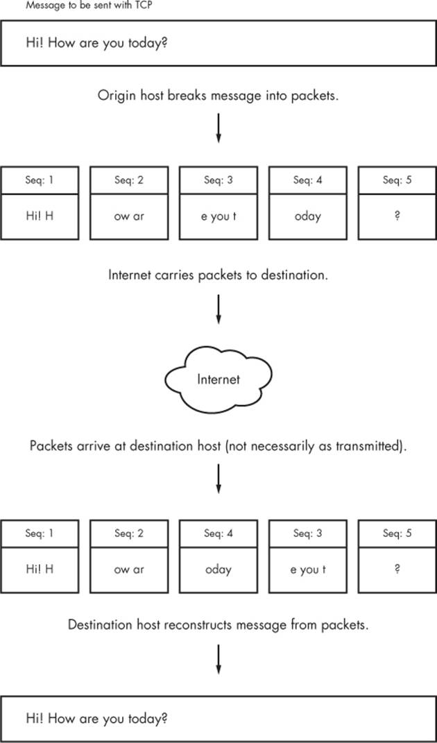
Figure 9-3. Sending a message with TCP

NOTE

The rest of this chapter deals with more advanced networking topics, such as network filtering and routers, as they relate to the lower network layers that we’ve already seen: physical, network, and transport. If you like, feel free to skip ahead to the next chapter to see the application layer where everything comes together in user space. You’ll see processes that actually use the network rather than just throwing around a bunch of addresses and packets.

9.15 Revisiting a Simple Local Network

We’re now going to look at additional components of the simple network introduced in 9.3 The Internet Layer. Recall that this network consists of one local area network as one subnet and a router that connects the subnet to the rest of the Internet. You’ll learn the following:

§ How a host on the subnet automatically gets its network configuration

§ How to set up routing

§ What a router really is

§ How to know which IP addresses to use for the subnet

§ How to set up firewalls to filter out unwanted traffic from the Internet

Let’s start by learning how a host on the subnet automatically gets its network configuration.

9.16 Understanding DHCP

When you set a network host to get its configuration automatically from the network, you’re telling it to use the Dynamic Host Configuration Protocol (DHCP) to get an IP address, subnet mask, default gateway, and DNS servers. Aside from not having to enter these parameters by hand, DHCP has other advantages for a network administrator, such as preventing IP address clashes and minimizing the impact of network changes. It’s very rare to see a modern network that doesn’t use DHCP.

For a host to get its configuration with DHCP, it must be able to send messages to a DHCP server on its connected network. Therefore, each physical network should have its own DHCP server, and on a simple network (such as the one in 9.3 The Internet Layer), the router usually acts as the DHCP server.

NOTE

When making an initial DHCP request, a host doesn’t even know the address of a DHCP server, so it broadcasts the request to all hosts (usually all hosts on its physical network).

When a machine asks a DHCP server for an IP address, it’s really asking for a lease on an address for a certain amount of time. When the lease is up, a client can ask to renew the lease.

9.16.1 The Linux DHCP Client

Although there are many different kinds of network manager systems, nearly all use the Internet Software Consortium (ISC) dhclient program to do the actual work. You can test dhclient by hand on the command line, but before doing so you must remove any default gateway route. To run the test, simply specify the network interface name (here, it’s eth0):

# dhclient eth0

Upon startup, dhclient stores its process ID in /var/run/dhclient.pid and its lease information in /var/state/dhclient.leases.

9.16.2 Linux DHCP Servers

You can task a Linux machine with running a DHCP server, which provides a good amount of control over the addresses that it gives out. However, unless you’re administering a large network with many subnets, you’re probably better off using specialized router hardware that includes built-in DHCP servers.

Probably the most important thing to know about DHCP servers is that you want only one running on the same subnet in order to avoid problems with clashing IP addresses or incorrect configurations.

9.17 Configuring Linux as a Router

Routers are essentially just computers with more than one physical network interface. You can easily configure a Linux machine as a router.

For example, say you have two LAN subnets, 10.23.2.0/24 and 192.168.45.0/24. To connect them, you have a Linux router machine with three network interfaces: two for the LAN subnets and one for an Internet uplink, as shown in Figure 9-4. As you can see, this doesn’t look very different from the simple network example that we’ve used in the rest of this chapter.

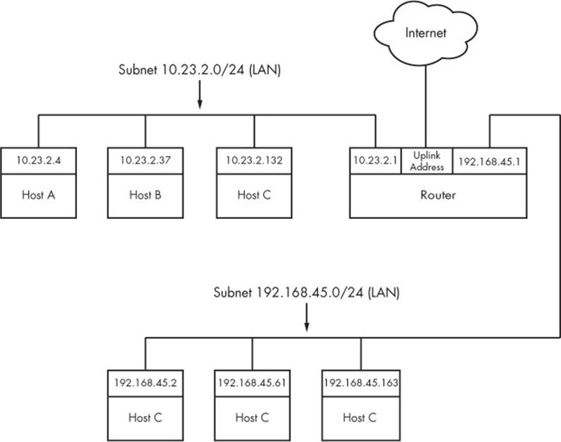
Figure 9-4. Two subnets joined with a router

The router’s IP addresses for the LAN subnets are 10.23.2.1 and 192.168.45.1. When those addresses are configured, the routing table looks something like this (the interface names might vary in practice; ignore the Internet uplink for now):

Destination Gateway Genmask Flags Metric Ref Use Iface

10.23.2.0 0.0.0.0 255.255.255.0 U 0 0 0 eth0

192.168.45.0 0.0.0.0 255.255.255.0 U 0 0 0 eth1

Now let’s say that the hosts on each subnet have the router as their default gateway (10.23.2.1 for 10.23.2.0/24 and 192.168.45.1 for 192.168.45.0/24). If 10.23.2.4 wants to send a packet to anything outside of 10.23.2.0/24, it passes the packet to 10.23.2.1. For example, to send a packet from 10.23.2.4 (Host A) to 192.168.45.61 (Host E), the packet goes to 10.23.2.1 (the router) via its eth0 interface, then back out through the router’s eth1 interface.

However, by default, the Linux kernel does not automatically move packets from one subnet to another. To enable this basic routing function, you need to enable IP forwarding in the router’s kernel with this command:

# sysctl -w net.ipv4.ip_forward

As soon as you enter this command, the machine should start routing packets between the two subnets, assuming that the hosts on those subnets know to send their packets to the router you just created.

To make this change permanent upon reboot, you can add it to your /etc/sysctl.conf file. Depending on your distribution, you may have the option to put it into a file in /etc/sysctl.d so that distribution updates won’t overwrite your changes.

9.17.1 Internet Uplinks

When the router also has the third network interface with an Internet uplink, this same setup allows Internet access for all hosts on both subnets because they’re configured to use the router as the default gateway. But that’s where things get more complicated. The problem is that certain IP addresses such as 10.23.2.4 are not actually visible to the whole Internet; they’re on so-called private networks. To provide for Internet connectivity, you must set up a feature called Network Address Translation (NAT) on the router. The software on nearly all specialized routers does this, so there’s nothing out of the ordinary here, but let’s examine the problem of private networks in a bit more detail.

9.18 Private Networks

Say you decide to build your own network. You have your machines, router, and network hardware ready. Given what you know about a simple network so far, your next question is “What IP subnet should I use?”

If you want a block of Internet addresses that every host on the Internet can see, you can buy one from your ISP. However, because the range of IPv4 addresses is very limited, this costs a a lot and isn’t useful for much more than running a server that the rest of the Internet can see. Most people don’t really need this kind of service because they access the Internet as a client.

The conventional, inexpensive alternative is to pick a private subnet from the addresses in the RFC 1918/6761 Internet standards documents, shown in Table 9-2.

Table 9-2. Private Networks Defined by RFC 1918 and 6761

You can carve up private subnets as you wish. Unless you plan to have more than 254 hosts on a single network, pick a small subnet like 10.23.2.0/24, as we’ve been using throughout this chapter. (Networks with this netmask are sometimes called class C subnets. Although the term is technically somewhat obsolete, it’s still useful.)

What’s the catch? Hosts on the real Internet know nothing about private subnets and will not send packets to them, so without some help, hosts on private subnets cannot talk to the outside world. A router connected to the Internet (with a true, nonprivate address) needs to have some way to fill in the gap between that connection and the hosts on a private network.

9.19 Network Address Translation (IP Masquerading)

NAT is the most commonly used way to share a single IP address with a private network, and it’s nearly universal in home and small office networks. In Linux, the variant of NAT that most people use is known as IP masquerading.

The basic idea behind NAT is that the router doesn’t just move packets from one subnet to another; it transforms them as it moves them. Hosts on the Internet know how to connect to the router, but they know nothing about the private network behind it. The hosts on the private network need no special configuration; the router is their default gateway.

The system works roughly like this:

1. A host on the internal private network wants to make a connection to the outside world, so it sends its connection request packets through the router.

2. The router intercepts the connection request packet rather than passing it out to the Internet (where it would get lost because the public Internet knows nothing about private networks).

3. The router determines the destination of the connection request packet and opens its own connection to the destination.

4. When the router obtains the connection, it fakes a “connection established” message back to the original internal host.

5. The router is now the middleman between the internal host and the destination. The destination knows nothing about the internal host; the connection on the remote host looks like it came from the router.

This isn’t quite as simple as it sounds. Normal IP routing knows only source and destination IP addresses in the Internet layer. However, if the router dealt only with the Internet layer, each host on the internal network could establish only one connection to a single destination at one time (among other limitations), because there is no information in the Internet layer part of a packet to distinguish multiple requests from the same host to the same destination. Therefore, NAT must go beyond the Internet layer and dissect packets to pull out more identifying information, particularly the UDP and TCP port numbers from the transport layers. UDP is fairly easy because there are ports but no connections, but the TCP transport layer is complex.

In order to set up a Linux machine to perform as a NAT router, you must activate all of the following inside the kernel configuration: network packet filtering (“firewall support”), connection tracking, IP tables support, full NAT, and MASQUERADE target support. Most distribution kernels come with this support.

Next you need to run some complex-looking iptables commands to make the router perform NAT for its private subnet. Here’s an example that applies to an internal Ethernet network on eth1 sharing an external connection at eth0 (you’ll learn more about the iptables syntax in 9.21 Firewalls):

# sysctl -w net.ipv4.ip_forward

# iptables -P FORWARD DROP

# iptables -t nat -A POSTROUTING -o eth0 -j MASQUERADE

# iptables -A FORWARD -i eth0 -o eth1 -m state --state ESTABLISHED,RELATED -j ACCEPT

# iptables -A FORWARD -i eth1 -o eth0 -j ACCEPT

NOTE

Although NAT works well in practice, remember that it’s essentially a hack used to extend the lifetime of the IPv4 address space. In a perfect world, we would all be using IPv6 (the next-generation Internet) and using its larger and more sophisticated address space without any pain.

You likely won’t ever need to use the commands above unless you’re developing your own software, especially with so much special-purpose router hardware available. But the role of Linux in a network doesn’t end here.

9.20 Routers and Linux

In the early days of broadband, users with less demanding needs simply connected their machine directly to the Internet. But it didn’t take long for many users to want to share a single broadband connection with their own networks, and Linux users in particular would often set up an extra machine to use as a router running NAT.

Manufacturers responded to this new market by offering specialized router hardware consisting of an efficient processor, some flash memory, and several network ports—with enough power to manage a typical simple network, run important software such as a DHCP server, and use NAT. When it came to software, many manufacturers turned to Linux to power their routers. They added the necessary kernel features, stripped down the user-space software, and created GUI-based administration interfaces.

Almost as soon as the first of these routers appeared, many people became interested in digging deeper into the hardware. One manufacturer, Linksys, was required to release the source code for its software under the terms of the license of one its components, and soon specialized Linux distributions such as OpenWRT appeared for routers. (The “WRT” in these names came from the Linksys model number.)

Aside from the hobbyist aspect, there are good reasons to use these distributions: They’re often more stable than the manufacturer firmware, especially on older router hardware, and they typically offer additional features. For example, to bridge a network with a wireless connection, many manufacturers require you to buy matching hardware, but with OpenWRT installed, the manufacturer and age of the hardware don’t really matter. This is because you’re using a truly open operating system on the router that doesn’t care what hardware you use as long as your hardware is supported.

You can use much of the knowledge in this book to examine the internals of custom Linux firmware, though you’ll encounter differences, especially when logging in. As with many embedded systems, open firmware tends to use BusyBox to provide many shell features. BusyBox is a single executable program that offers limited functionality for many Unix commands such as the shell, ls, grep, cat, and more. (This saves a significant amount of memory.) In addition, the boot-time init tends to be very simple on embedded systems. However, you typically won’t find these limitations to be a problem, because custom Linux firmware often includes a web administration interface similar to what you’d see from a manufacturer.

9.21 Firewalls

Routers in particular should always include some kind of firewall to keep undesirable traffic out of your network. A firewall is a software and/or hardware configuration that usually sits on a router between the Internet and a smaller network, attempting to ensure that nothing “bad” from the Internet harms the smaller network. You can also set up firewall features for each machine where the machine screens all of its incoming and outgoing data at the packet level (as opposed to the application layer, where server programs usually try to perform some access control of their own). Firewalling on individual machines is sometimes called IP filtering.

A system can filter packets when it

§ receives a packet,

§ sends a packet, or

§ forwards (routes) a packet to another host or gateway.

With no firewalling in place, a system just processes packets and sends them on their way. Firewalls put checkpoints for packets at the points of data transfer identified above. The checkpoints drop, reject, or accept packets, usually based on some of these criteria:

§ The source or destination IP address or subnet

§ The source or destination port (in the transport layer information)

§ The firewall’s network interface

Firewalls provide an opportunity to work with the subsystem of the Linux kernel that processes IP packets. Let’s look at that now.

9.21.1 Linux Firewall Basics

In Linux, you create firewall rules in a series known as a chain. A set of chains makes up a table. As a packet moves through the various parts of the Linux networking subsystem, the kernel applies the rules in certain chains to the packets. For example, after receiving a new packet from the physical layer, the kernel activates rules in chains corresponding to input.

All of these data structures are maintained by the kernel. The whole system is called iptables, with an iptables user-space command to create and manipulate the rules.

NOTE

There is a newer system called nftables that has a goal of replacing iptables, but as of this writing, iptables is the dominant system for firewalls.

Because there can be many tables—each with their own sets of chains, each of which can contain many rules—packet flow can become quite complicated. However, you’ll normally work primarily with a single table named filter that controls basic packet flow. There are three basic chains in the filter table: INPUT for incoming packets, OUTPUT for outgoing packets, and FORWARD for routed packets.

Figure 9-5 and Figure 9-6 show simplified flowcharts for where rules are applied to packets in the filter table. There are two figures because packets can either come into the system from a network interface (Figure 9-5) or be generated by a local process (Figure 9-6). As you can see, an incoming packet from the network can be consumed by a user process and may not reach the FORWARD chain or the OUTPUT chain. Packets generated by user processes won’t reach the INPUT or FORWARD chains.

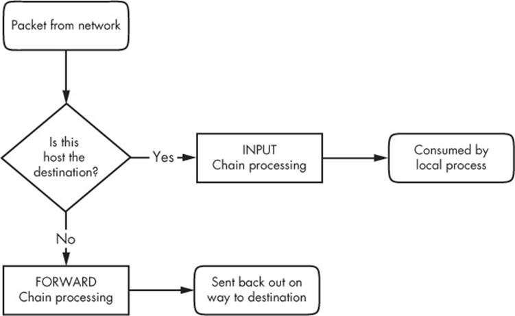
Figure 9-5. Chain-processing sequence for incoming packets from a network

Figure 9-6. Chain-processing sequence for incoming packets from a local process

This gets more complicated because there are many steps along the way other than just these three chains. For example, packets are subject to PREROUTING and POSTROUTING chains, and chain processing can also occur at any of the three lower network levels. For a big diagram for everything that’s going on, search the Internet for “Linux netfilter packet flow,” but remember that these diagrams try to include every possible scenario for packet input and flow. It often helps to break the diagrams down by packet source, as in Figure 9-5 and Figure 9-6.

9.21.2 Setting Firewall Rules

Let’s look at how the IP tables system works in practice. Start by viewing the current configuration with this command:

# iptables -L

The output is usually an empty set of chains, as follows:

Chain INPUT (policy ACCEPT)

target prot opt source destination

Chain FORWARD (policy ACCEPT)

target prot opt source destination

Chain OUTPUT (policy ACCEPT)

target prot opt source destination

Each firewall chain has a default policy that specifies what to do with a packet if no rule matches the packet. The policy for all three chains in this example is ACCEPT, meaning that the kernel allows the packet to pass through the packet-filtering system. The DROP policy tells the kernel to discard the packet. To set the policy on a chain, use iptables -P like this:

# iptables -P FORWARD DROP

WARNING

Don’t do anything rash with the policies on your machine until you’ve read through the rest of this section.

Say that someone at 192.168.34.63 is annoying you. To prevent them from talking to your machine, run this command:

# iptables -A INPUT -s 192.168.34.63 -j DROP

The -A INPUT parameter appends a rule to the INPUT chain. The -s 192.168.34.63 part specifies the source IP address in the rule, and -j DROP tells the kernel to discard any packet matching the rule. Therefore, your machine will throw out any packet coming from 192.168.34.63.

To see the rule in place, run iptables -L:

Chain INPUT (policy ACCEPT)

target prot opt source destination

DROP all -- 192.168.34.63 anywhere

Unfortunately, your friend at 192.168.34.63 has told everyone on his subnet to open connections to your SMTP port (TCP port 25). To get rid of that traffic as well, run

# iptables -A INPUT -s 192.168.34.0/24 -p tcp --destination-port 25 -j DROP

This example adds a netmask qualifier to the source address as well as -p tcp to specify TCP packets only. A further restriction, --destination-port 25, says that the rule should only apply to traffic to port 25. The IP table list for INPUT now looks like this:

Chain INPUT (policy ACCEPT)

target prot opt source destination

DROP all -- 192.168.34.63 anywhere

DROP tcp -- 192.168.34.0/24 anywhere tcp dpt:smtp

All is well until you hear from someone you know at 192.168.34.37 saying that they can’t send you email because you blocked their machine. Thinking that this is a quick fix, you run this command:

# iptables -A INPUT -s 192.168.34.37 -j ACCEPT

However, it doesn’t work. To see why, look at the new chain:

Chain INPUT (policy ACCEPT)

target prot opt source destination

DROP all -- 192.168.34.63 anywhere

DROP tcp -- 192.168.34.0/24 anywhere tcp dpt:smtp

ACCEPT all -- 192.168.34.37 anywhere

The kernel reads the chain from top to bottom, using the first rule that matches.

The first rule does not match 192.168.34.37, but the second does, because it applies to all hosts from 192.168.34.1 to 192.168.34.254 and this second rule says to drop packets. When a rule matches, the kernel carries out the action and looks no further down in the chain. (You might notice that 192.168.34.37 can send packets to any port on your machine except port 25 because the second rule only applies to port 25.)

The solution is to move the third rule to the top. First, delete the third rule with this command:

# iptables -D INPUT 3

Then insert that rule at the top of the chain with iptables -I:

# iptables -I INPUT -s 192.168.34.37 -j ACCEPT

To insert a rule elsewhere in a chain, put the rule number after the chain name (for example, iptables -I INPUT 4 ...).

9.21.3 Firewall Strategies

Although the tutorial above showed you how to insert rules and how the kernel processes IP chains, we haven’t seen firewall strategies that actually work. Let’s talk about that now.

There are two basic kinds of firewall scenarios: one for protecting individual machines (where you set rules in each machine’s INPUT chain) and one for protecting a network of machines (where you set rules in the router’s FORWARD chain). In both cases, you can’t have serious security if you use a default policy of ACCEPT and continuously insert rules to drop packets from sources that start to send bad stuff. You must allow only the packets that you trust and deny everything else.

For example, say your machine has an SSH server on TCP port 22. There’s no reason for any random host to initiate a connection to any other port on your machine, and you shouldn’t give any such host a chance. To set that up, first set the INPUT chain policy to DROP:

# iptables -P INPUT DROP

To enable ICMP traffic (for ping and other utilities), use this line:

# iptables -A INPUT -p icmp -j ACCEPT

Make sure that you can receive packets you send to both your own network IP address and 127.0.0.1 (localhost). Assuming your host’s IP address is my_addr, do this:

# iptables -A INPUT -s 127.0.0.1 -j ACCEPT

# iptables -A INPUT -s my_addr -j ACCEPT

If you control your entire subnet (and trust everything on it), you can replace my_addr with your subnet address and subnet mask, for example, 10.23.2.0/24.

Now, although you still want to deny incoming TCP connections, you still need to make sure that your host can make TCP connections to the outside world. Because all TCP connections start with a SYN (connection request) packet, if you let all TCP packets through that aren’t SYN packets, you’re still okay:

# iptables -A INPUT -p tcp '!' --syn -j ACCEPT

Next, if you’re using remote UDP-based DNS, you must accept traffic from your name server so that your machine can look up names with DNS. Do this for all DNS servers in /etc/resolv.conf. Use this command (where the name server’s address is ns_addr):

# iptables -A INPUT -p udp --source-port 53 -s ns_addr -j ACCEPT

And finally, allow SSH connections from anywhere:

# iptables -A INPUT -p tcp --destination-port 22 -j ACCEPT

The preceding iptables settings work for many situations, including any direct connection (especially broadband) where an intruder is much more likely to port-scan your machine. You could also adapt these settings for a firewalling router by using the FORWARD chain instead of INPUT and using source and destination subnets where appropriate. For more advanced configurations, you may find a configuration tool such as Shorewall to be helpful.

This discussion has only touched on security policy. Remember that the key idea is to permit only the things that you find acceptable, not to try to find and execute the bad stuff. Furthermore, IP firewalling is only one piece of the security picture. (You’ll see more in the next chapter.)

9.22 Ethernet, IP, and ARP

There is one interesting basic detail in the implementation of IP over Ethernet that we have yet to cover. Recall that a host must place an IP packet inside an Ethernet frame in order to transmit the packet across the physical layer to another host. Recall, too, that frames themselves do not include IP address information; they use MAC (hardware) addresses. The question is this: When constructing the Ethernet frame for an IP packet, how does the host know which MAC address corresponds to the destination IP address?

We don’t normally think about this question much because networking software includes an automatic system of looking up MAC addresses called Address Resolution Protocol (ARP). A host using Ethernet as its physical layer and IP as the network layer maintains a small table called anARP cache that maps IP addresses to MAC addresses. In Linux, the ARP cache is in the kernel. To view your machine’s ARP cache, use the arp command. (As with many other network commands, the -n option here disables reverse DNS lookups.)

$ arp -n

Address Hwtype Hwaddr Flags Mask Iface

10.1.2.141 ether 00:11:32:0d:ca:82 C eth0

10.1.2.1 ether 00:24:a5:b5:a0:11 C eth0

10.1.2.50 ether 00:0c:41:f6:1c:99 C eth0

When a machine boots, its ARP cache is empty. So how do these MAC addresses get in the cache? It all starts when the machine wants to send a packet to another host. If a target IP address is not in an ARP cache, the following steps occur:

1. The origin host creates a special Ethernet frame containing an ARP request packet for the MAC address that corresponds to the target IP address.

2. The origin host broadcasts this frame to the entire physical network for the target’s subnet.

3. If one of the other hosts on the subnet knows the correct MAC address, it creates a reply packet and frame containing the address and sends it back to the origin. Often, the host that replies is the target host and is simply replying with its own MAC address.

4. The origin host adds the IP-MAC address pair to the ARP cache and can proceed.

NOTE

Remember that ARP only applies to machines on local subnets (refer to 9.4 Routes and the Kernel Routing Table to see your local subnets). To reach destinations outside your subnet, your host sends the packet to the router, and it’s someone else’s problem after that. Of course, your host still needs to know the MAC address for the router, and it can use ARP to find it.

The only real problem you can have with ARP is that your system’s cache can get out-of-date if you’re moving an IP address from one network interface card to another because the cards have different MAC addresses (for example, when testing a machine). Unix systems invalidate ARP cache entries if there’s no activity after a while, so there shouldn’t be any trouble other than a small delay for invalidated data, but you can delete an ARP cache entry immediately with this command:

# arp -d host

You can also view the ARP cache for a single network interface with

$ arp -i interface

The arp(8) manual page explains how to manually set ARP cache entries, but you shouldn’t need to do this.

NOTE

Don’t confuse ARP with Reverse Address Resolution Protocol (RARP). RARP transforms a MAC address back to a hostname or IP address. Before DHCP became popular, some diskless workstations and other devices used RARP to get their configuration, but RARP is rare today.

9.23 Wireless Ethernet

In principle, wireless Ethernet (“WiFi”) networks aren’t much different from wired networks. Much like any wired hardware, they have MAC addresses and use Ethernet frames to transmit and receive data, and as a result the Linux kernel can talk to a wireless network interface much as it would a wired network interface. Everything at the network layer and above is the same; the main differences are additional components in the physical layer such as frequencies, network IDs, security, and so on.

Unlike wired network hardware, which is very good at automatically adjusting to nuances in the physical setup without much fuss, wireless network configuration is much more open-ended. To get a wireless interface working properly, Linux needs additional configuration tools.

Let’s take a quick look at the additional components of wireless networks.

§ Transmission details. These are physical characteristics, such as the radio frequency.

§ Network identification. Because more than one wireless network can share the same basic medium, you have to be able to distinguish between them. The SSID (Service Set Identifier, also known as the “network name”) is the wireless network identifier.

§ Management. Although it’s possible to configure wireless networking to have hosts talk directly to each other, most wireless networks are managed by one or more access points that all traffic goes through. Access points often bridge a wireless network with a wired network, making both appear as one single network.

§ Authentication. You may want to restrict access to a wireless network. To do so, you can configure access points to require a password or other authentication key before they’ll even talk to a client.

§ Encryption. In addition to restricting the initial access to a wireless network, you normally want to encrypt all traffic that goes out across radio waves.

The Linux configuration and utilities that handle these components are spread out over a number of areas. Some are in the kernel: Linux features a set of wireless extensions that standardize user-space access to hardware. As far as user space goes, wireless configuration can get complicated, so most people prefer to use GUI frontends, such as the desktop applet for NetworkManager, to get things working. Still, it’s worth looking at a few of the things happening behind the scenes.

9.23.1 iw

You can view and change kernel space device and network configuration with a utility called iw. To use iw, you normally need to know the network interface name for the device, such as wlan0. Here’s an example that dumps a scan of available wireless networks. (Expect a lot of output if you’re in an urban area.)

# iw dev wlan0 scan

NOTE

The network interface must be up for this command to work (if it’s not, run ifconfig wlan0 up), but you don’t need to configure any network layer parameters, such as an IP address.

If the network interface has joined a wireless network, you can view the network details like this:

# iw dev wlan0 link

The MAC address in the output of this command is from the access point that you’re currently talking to.

NOTE

The iw command distinguishes between physical device names such as phy0 and network interface names such as wlan0 and allows you to change various settings for each. You can even create more than one network interface for a single physical device. However, in nearly all basic cases, you’ll just use the network interface name.

Use iw to connect a network interface to an unsecured wireless network as follows:

# iw wlan0 connect network_name

Connecting to secured networks is a different story. For the rather insecure Wired Equivalent Privacy (WEP) system, you can use the keys parameter with the iw connect command. However, you shouldn’t use WEP if you’re serious about security.

9.23.2 Wireless Security

For most wireless security setups, Linux relies on a daemon called wpa_supplicant to manage both authentication and encryption for a wireless network interface. This daemon can handle both WPA (WiFi Protected Access) and WPA2 schemes of authentication, as well as nearly any kind of encryption technique used on wireless networks. When the daemon first starts, it reads a configuration file (by default, /etc/wpa_supplicant.conf) and attempts to identify itself to an access point and establish communication based on a given network name. The system is well documented; in particular, the wpa_supplicant(1) and wpa_supplicant.conf(5) manual pages are very detailed.

Running the daemon by hand every time you want to establish a connection is a lot of work. In fact, just creating the configuration file is tedious due to the number of possible options. To make matters worse, all of the work of running iw and wpa_supplicant simply allows your system to join a wireless physical network; it doesn’t even set up the network layer. And that’s where automatic network configuration managers such as NetworkManager take a lot of pain out of the process. Although they don’t do any of the work on their own, they know the correct sequence and required configuration for each step toward getting a wireless network operational.

9.24 Summary

You can now see that understanding the positions and roles of the various network layers is critical to understanding how Linux networking operates and how to perform network configuration. Although we’ve covered only the basics, more advanced topics in the physical, network, and transport layers bear similarities to what you’ve seen. Layers themselves are often subdivided, as you just saw with the various pieces of the physical layer in a wireless network.

A substantial amount of action that you’ve seen in this chapter happens in the kernel, with some basic user-space control utilities to manipulate the kernel’s internal data structures (such as routing tables). This is the traditional way of working with the network. However, as with many of the topics discussed in this book, some tasks aren’t suitable for the kernel due to their complexity and need for flexibility, and that’s where user-space utilities take over. In particular, NetworkManager monitors and queries the kernel and then manipulates the kernel configuration. Another example is support for dynamic routing protocols such as Border Gateway Protocol (BGP), which is used in large Internet routers.

But you’re probably a little bit bored with network configuration by now. Let’s turn to using the network—the application layer.