How Linux Works: What Every Superuser Should Know (2015)
Chapter 4. Disks and Filesystems
In Chapter 3, we discussed some of the top-level disk devices that the kernel makes available. In this chapter, we’ll discuss in detail how to work with disks on a Linux system. You’ll learn how to partition disks, create and maintain the filesystems that go inside disk partitions, and work with swap space.
Recall that disk devices have names like /dev/sda, the first SCSI subsystem disk. This kind of block device represents the entire disk, but there are many different components and layers inside a disk.
Figure 4-1 illustrates the schematic of a typical Linux disk (note that the figure is not to scale). As you progress through this chapter, you’ll learn where each piece fits in.
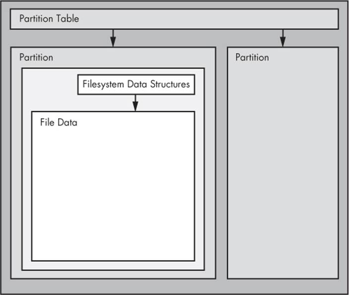
Figure 4-1. Typical Linux disk schematic
Partitions are subdivisions of the whole disk. On Linux, they’re denoted with a number after the whole block device, and therefore have device names such as /dev/sda1 and /dev/sdb3. The kernel presents each partition as a block device, just as it would an entire disk. Partitions are defined on a small area of the disk called a partition table.
NOTE
Multiple data partitions were once common on systems with large disks because older PCs could boot only from certain parts of the disk. Also, administrators used partitions to reserve a certain amount of space for operating system areas; for example, they didn’t want users to be able to fill up the entire system and prevent critical services from working. This practice is not unique to Unix; you’ll still find many new Windows systems with several partitions on a single disk. In addition, most systems have a separate swap partition.
Although the kernel makes it possible for you to access both an entire disk and one of its partitions at the same time, you would not normally do so, unless you were copying the entire disk.
The next layer after the partition is the filesystem, the database of files and directories that you’re accustomed to interacting with in user space. We’ll explore filesystems in 4.2 Filesystems.
As you can see in Figure 4-1, if you want to access the data in a file, you need to get the appropriate partition location from the partition table and then search the filesystem database on that partition for the desired file data.
To access data on a disk, the Linux kernel uses the system of layers shown in Figure 4-2. The SCSI subsystem and everything else described in 3.6 In-Depth: SCSI and the Linux Kernel are represented by a single box. (Notice that you can work with the disk through the filesystem as well as directly through the disk devices. You’ll do both in this chapter.)
To get a handle on how everything fits together, let’s start at the bottom with partitions.
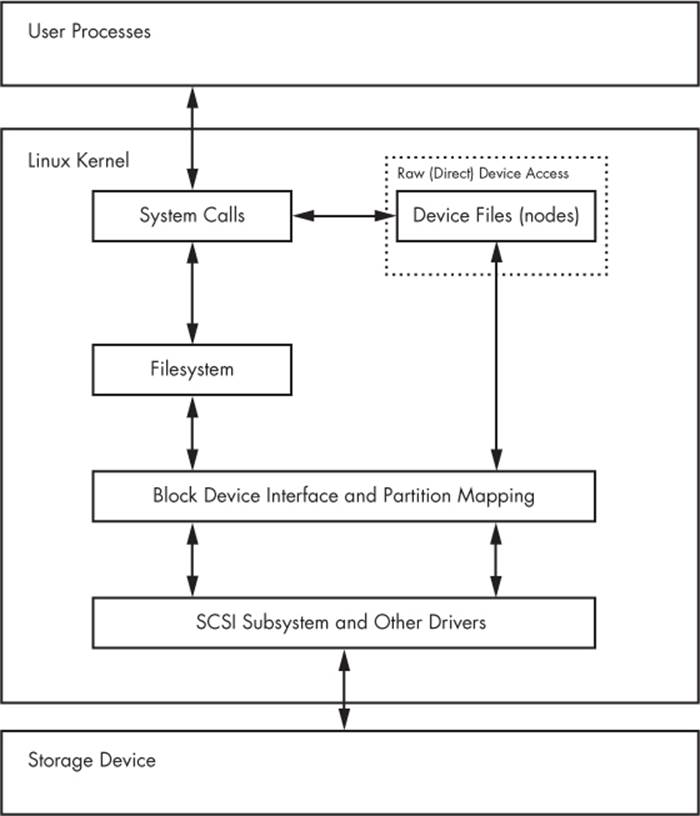
Figure 4-2. Kernel schematic for disk access
4.1 Partitioning Disk Devices
There are many kinds of partition tables. The traditional table is the one found inside the Master Boot Record (MBR). A newer standard starting to gain traction is the Globally Unique Identifier Partition Table (GPT).
Here is an overview of the many Linux partitioning tools available:
§ parted A text-based tool that supports both MBR and GPT.
§ gparted A graphical version of parted.
§ fdisk The traditional text-based Linux disk partitioning tool. fdisk does not support GPT.
§ gdisk A version of fdisk that supports GPT but not MBR.
Because it supports both MBR and GPT, we’ll use parted in this book. However, many people prefer the fdisk interface, and there’s nothing wrong with that.
NOTE
Although parted can create and resize filesystems, you shouldn’t use it for filesystem manipulation because you can easily get confused. There is a critical difference between partitioning and filesystem manipulation. The partition table defines simple boundaries on the disk, whereas a filesystem is a much more involved data system. For this reason, we’ll use parted for partitioning but use separate utilities for creating filesystems (see 4.2.2 Creating a Filesystem). Even the parted documentation encourages you to create filesystems separately.
4.1.1 Viewing a Partition Table
You can view your system’s partition table with parted -l. Here is sample output from two disk devices with two different kinds of partition tables:
# parted -l
Model: ATA WDC WD3200AAJS-2 (scsi)
Disk /dev/sda: 320GB
Sector size (logical/physical): 512B/512B
Partition Table: msdos
Number Start End Size Type File system Flags
1 1049kB 316GB 316GB primary ext4 boot
2 316GB 320GB 4235MB extended
5 316GB 320GB 4235MB logical linux-swap(v1)
Model: FLASH Drive UT_USB20 (scsi)
Disk /dev/sdf: 4041MB
Sector size (logical/physical): 512B/512B
Partition Table: gpt
Number Start End Size File system Name Flags
1 17.4kB 1000MB 1000MB myfirst
2 1000MB 4040MB 3040MB mysecond
The first device, /dev/sda, uses the traditional MBR partition table (called “msdos” by parted), and the second contains a GPT table. Notice that there are different parameters for each partition table, because the tables themselves are different. In particular, there is no Name column for the MBR table because names don’t exist under that scheme. (I arbitrarily chose the names myfirst and mysecond in the GPT table.)
The MBR table in this example contains primary, extended, and logical partitions. A primary partition is a normal subdivision of the disk; partition 1 is such a partition. The basic MBR has a limit of four primary partitions, so if you want more than four, you designate one partition as anextended partition. Next, you subdivide the extended partition into logical partitions that the operating system can use as it would any other partition. In this example, partition 2 is an extended partition that contains logical partition 5.
NOTE
The filesystem that parted lists is not necessarily the system ID field defined in most MBR entries. The MBR system ID is just a number; for example, 83 is a Linux partition and 82 is Linux swap. Therefore, parted attempts to determine a filesystem on its own. If you absolutely must know the system ID for an MBR, use fdisk -l.
Initial Kernel Read
When initially reading the MBR table, the Linux kernel produces the following debugging output (remember that you can view this with dmesg):
sda: sda1 sda2 < sda5 >
The sda2 < sda5 > output indicates that /dev/sda2 is an extended partition containing one logical partition, /dev/sda5. You’ll normally ignore extended partitions because you’ll typically want to access only the logical partitions inside.
4.1.2 Changing Partition Tables
Viewing partition tables is a relatively simple and harmless operation. Altering partition tables is also relatively easy, but there are risks involved in making this kind of change to the disk. Keep the following in mind:
§ Changing the partition table makes it quite difficult to recover any data on partitions that you delete because it changes the initial point of reference for a filesystem. Make sure that you have a backup if the disk you’re partitioning contains critical data.
§ Ensure that no partitions on your target disk are currently in use. This is a concern because most Linux distributions automatically mount any detected filesystem. (See 4.2.3 Mounting a Filesystem for more on mounting and unmounting.)
When you’re ready, choose your partitioning program. If you’d like to use parted, you can use the command-line parted utility or a graphical interface such as gparted; for an fdisk-style interface, use gdisk if you’re using GPT partitioning. These utilities all have online help and are easy to learn. (Try using them on a flash device or something similar if you don’t have any spare disks.)
That said, there is a major difference in the way that fdisk and parted work. With fdisk, you design your new partition table before making the actual changes to the disk; fdisk only makes the changes as you exit the program. But with parted, partitions are created, modified, and removed as you issue the commands. You don’t get the chance to review the partition table before you change it.
These differences are also important to understanding how these two utilities interact with the kernel. Both fdisk and parted modify the partitions entirely in user space; there is no need to provide kernel support for rewriting a partition table because user space can read and modify all of a block device.
Eventually, though, the kernel must read the partition table in order to present the partitions as block devices. The fdisk utility uses a relatively simple method: After modifying the partition table, fdisk issues a single system call on the disk to tell the kernel that it should reread the partition table. The kernel then generates debugging output that you can view with dmesg. For example, if you create two partitions on /dev/sdf, you’ll see this:
sdf: sdf1 sdf2
In comparison, the parted tools do not use this disk-wide system call. Instead, they signal the kernel when individual partitions are altered. After processing a single partition change, the kernel does not produce the preceding debugging output.
There are a few ways to see the partition changes:
§ Use udevadm to watch the kernel event changes. For example, udevadm monitor --kernel will show the old partition devices being removed and the new ones being added.
§ Check /proc/partitions for full partition information.
§ Check /sys/block/device/ for altered partition system interfaces or /dev for altered partition devices.
If you absolutely must be sure that you have modified a partition table, you can perform the old-style system call that fdisk uses by using the blockdev command. For example, to force the kernel to reload the partition table on /dev/sdf, run this:
# blockdev --rereadpt /dev/sdf
At this point, you have all you need to know about partitioning disks. However, if you’re interested in learning a few more details about disks, read on. Otherwise, skip ahead to 4.2 Filesystems to learn about putting a file-system on the disk.
4.1.3 Disk and Partition Geometry
Any device with moving parts introduces complexity into a software system because there are physical elements that resist abstraction. A hard disk is no exception; even though you can think of a hard disk as a block device with random access to any block, there are serious performance consequences if you aren’t careful about how you lay out data on the disk. Consider the physical properties of the simple single-platter disk illustrated in Figure 4-3.
The disk consists of a spinning platter on a spindle, with a head attached to a moving arm that can sweep across the radius of the disk. As the disk spins underneath the head, the head reads data. When the arm is in one position, the head can only read data from a fixed circle. This circle is called a cylinder because larger disks have more than one platter, all stacked and spinning around the same spindle. Each platter can have one or two heads, for the top and/or bottom of the platter, and all heads are attached to the same arm and move in concert. Because the arm moves, there are many cylinders on the disk, from small ones around the center to large ones around the periphery of the disk. Finally, you can divide a cylinder into slices called sectors. This way of thinking about the disk geometry is called CHS, for cylinder-head-sector.
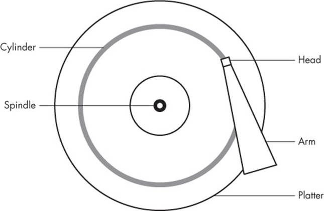
Figure 4-3. Top-down view of a hard disk
NOTE
A track is a part of a cylinder that a single head accesses, so in Figure 4-3, a cylinder is also a track. You probably don’t need to worry about tracks.
The kernel and the various partitioning programs can tell you what a disk reports as its number of cylinders (and sectors, which are slices of cylinders). However, on a modern hard disk, the reported values are fiction! The traditional addressing scheme that uses CHS doesn’t scale with modern disk hardware, nor does it account for the fact that you can put more data into outer cylinders than inner cylinders. Disk hardware supports Logical Block Addressing (LBA) to simply address a location on the disk by a block number, but remnants of CHS remain. For example, the MBR partition table contains CHS information as well as LBA equivalents, and some boot loaders are still dumb enough to believe the CHS values (don’t worry—most Linux boot loaders use the LBA values).
Nevertheless, the idea of cylinders has been important to partitioning because cylinders are ideal boundaries for partitions. Reading a data stream from a cylinder is very fast because the head can continuously pick up data as the disk spins. A partition arranged as a set of adjacent cylinders also allows for fast continuous data access because the head doesn’t need to move very far between cylinders.
Some partitioning programs complain if you don’t place your partitions precisely on cylinder boundaries. Ignore this; there’s little you can do because the reported CHS values of modern disks simply aren’t true. The disk’s LBA scheme ensures that your partitions are where they’re supposed to be.
4.1.4 Solid-State Disks (SSDs)
Storage devices with no moving parts, such as solid-state disks (SSDs), are radically different from spinning disks in terms of their access characteristics. For these, random access is not a problem because there’s no head to sweep across a platter, but certain factors affect performance.
One of the most significant factors affecting the performance of SSDs is partition alignment. When you read data from an SSD, you read it in chunks— typically 4096 bytes at a time—and the read must begin at a multiple of that same size. So if your partition and its data do not lie on a 4096-byte boundary, you may have to do two reads instead of one for small, common operations, such as reading the contents of a directory.
Many partitioning utilities (parted and gparted, for example) include functionality to put newly created partitions at the proper offsets from the beginning of the disks, so you may never need to worry about improper partition alignment. However, if you’re curious about where your partitions begin and just want to make sure that they begin on a boundary, you can easily find this information by looking in /sys/block. Here’s an example for a partition /dev/sdf2:
$ cat /sys/block/sdf/sdf2/start
1953126
This partition starts at 1,953,126 bytes from the beginning of the disk. Because this number is not divisible by 4,096, the partition would not be attaining optimal performance if it were on SSD.
4.2 Filesystems
The last link between the kernel and user space for disks is typically the file-system; this is what you’re accustomed to interacting with when you run commands such as ls and cd. As previously mentioned, the filesystem is a form of database; it supplies the structure to transform a simple block device into the sophisticated hierarchy of files and subdirectories that users can understand.
At one time, filesystems resided on disks and other physical media used exclusively for data storage. However, the tree-like directory structure and I/O interface of filesystems are quite versatile, so filesystems now perform a variety of tasks, such as the system interfaces that you see in /sysand /proc. Filesystems are also traditionally implemented in the kernel, but the innovation of 9P from Plan 9 (http://plan9.bell-labs.com/sys/doc/9.html) has inspired the development of user-space filesystems. The File System in User Space (FUSE) feature allows user-space filesystems in Linux.
The Virtual File System (VFS) abstraction layer completes the filesystem implementation. Much as the SCSI subsystem standardizes communication between different device types and kernel control commands, VFS ensures that all filesystem implementations support a standard interface so that user-space applications access files and directories in the same manner. VFS support has enabled Linux to support an extraordinarily large number of filesystems.
4.2.1 Filesystem Types
Linux filesystem support includes native designs optimized for Linux, foreign types such as the Windows FAT family, universal filesystems like ISO 9660, and many others. The following list includes the most common types of filesystems for data storage. The type names as recognized by Linux are in parentheses next to the filesystem names.
§ The Fourth Extended filesystem (ext4) is the current iteration of a line of filesystems native to Linux. The Second Extended filesystem (ext2) was a longtime default for Linux systems inspired by traditional Unix filesystems such as the Unix File System (UFS) and the Fast File System (FFS). The Third Extended filesystem (ext3) added a journal feature (a small cache outside the normal filesystem data structure) to enhance data integrity and hasten booting. The ext4 filesystem is an incremental improvement with support for larger files than ext2 or ext3 support and a greater number of subdirectories.
There is a certain amount of backward compatibility in the extended filesystem series. For example, you can mount ext2 and ext3 filesystems as each other, and you can mount ext2 and ext3 filesystems as ext4, but you cannot mount ext4 as ext2 or ext3.
§ ISO 9660 (iso9660) is a CD-ROM standard. Most CD-ROMs use some variety of the ISO 9660 standard.
§ FAT filesystems (msdos, vfat, umsdos) pertain to Microsoft systems. The simple msdos type supports the very primitive monocase variety in MS-DOS systems. For most modern Windows filesystems, you should use the vfat filesystem in order to get full access from Linux. The rarely used umsdos filesystem is peculiar to Linux. It supports Unix features such as symbolic links on top of an MS-DOS filesystem.
§ HFS+ (hfsplus) is an Apple standard used on most Macintosh systems.
Although the Extended filesystem series has been perfectly acceptable to most casual users, many advances have been made in filesystem technology that even ext4 cannot utilize due to the backward compatibility requirement. The advances are primarily in scalability enhancements pertaining to very large numbers of files, large files, and similar scenarios. New Linux filesystems, such as Btrfs, are under development and may be poised to replace the Extended series.
4.2.2 Creating a Filesystem
Once you’re done with the partitioning process described in 4.1 Partitioning Disk Devices, you’re ready to create filesystems. As with partitioning, you’ll do this in user space because a user-space process can directly access and manipulate a block device. The mkfs utility can create many kinds of filesystems. For example, you can create an ext4 partition on /dev/sdf2 with this command:
# mkfs -t ext4 /dev/sdf2
The mkfs program automatically determines the number of blocks in a device and sets some reasonable defaults. Unless you really know what you’re doing and feel like reading the documentation in detail, don’t change these.
When you create a filesystem, mkfs prints diagnostic output as it works, including output pertaining to the superblock. The superblock is a key component at the top level of the filesystem database, and it’s so important that mkfs creates a number of backups in case the original is destroyed. Consider recording a few of the superblock backup numbers when mkfs runs, in case you need to recover the superblock in the event of a disk failure (see 4.2.11 Checking and Repairing Filesystems).
WARNING
Filesystem creation is a task that you should only need to perform after adding a new disk or repartitioning an old one. You should create a filesystem just once for each new partition that has no preexisting data (or that has data that you want to remove). Creating a new filesystem on top of an existing filesystem will effectively destroy the old data.
It turns out that mkfs is only a frontend for a series of filesystem creation programs, mkfs.fs, where fs is a filesystem type. So when you run mkfs -t ext4, mkfs in turn runs mkfs.ext4.
And there’s even more indirection. Inspect the mkfs.* files behind the commands and you’ll see the following:
$ ls -l /sbin/mkfs.*
-rwxr-xr-x 1 root root 17896 Mar 29 21:49 /sbin/mkfs.bfs
-rwxr-xr-x 1 root root 30280 Mar 29 21:49 /sbin/mkfs.cramfs
lrwxrwxrwx 1 root root 6 Mar 30 13:25 /sbin/mkfs.ext2 -> mke2fs
lrwxrwxrwx 1 root root 6 Mar 30 13:25 /sbin/mkfs.ext3 -> mke2fs
lrwxrwxrwx 1 root root 6 Mar 30 13:25 /sbin/mkfs.ext4 -> mke2fs
lrwxrwxrwx 1 root root 6 Mar 30 13:25 /sbin/mkfs.ext4dev -> mke2fs
-rwxr-xr-x 1 root root 26200 Mar 29 21:49 /sbin/mkfs.minix
lrwxrwxrwx 1 root root 7 Dec 19 2011 /sbin/mkfs.msdos -> mkdosfs
lrwxrwxrwx 1 root root 6 Mar 5 2012 /sbin/mkfs.ntfs -> mkntfs
lrwxrwxrwx 1 root root 7 Dec 19 2011 /sbin/mkfs.vfat -> mkdosfs
As you can see, mkfs.ext4 is just a symbolic link to mke2fs. This is important to remember if you run across a system without a specific mkfs command or when you’re looking up the documentation for a particular filesystem. Each filesystem’s creation utility has its own manual page, like mke2fs(8). This shouldn’t be a problem on most systems, because accessing the mkfs.ext4(8) manual page should redirect you to the mke2fs(8) manual page, but keep it in mind.
4.2.3 Mounting a Filesystem
On Unix, the process of attaching a filesystem is called mounting. When the system boots, the kernel reads some configuration data and mounts root (/) based on the configuration data.
In order to mount a filesystem, you must know the following:
§ The filesystem’s device (such as a disk partition; where the actual file-system data resides).
§ The filesystem type.
§ The mount point—that is, the place in the current system’s directory hierarchy where the filesystem will be attached. The mount point is always a normal directory. For instance, you could use /cdrom as a mount point for CD-ROM devices. The mount point need not be directly below /; it may be anywhere on the system.
When mounting a filesystem, the common terminology is “mount a device on a mount point.” To learn the current filesystem status of your system, run mount. The output should look like this:
$ mount
/dev/sda1 on / type ext4 (rw,errors=remount-ro)
proc on /proc type proc (rw,noexec,nosuid,nodev)
sysfs on /sys type sysfs (rw,noexec,nosuid,nodev)
none on /sys/fs/fuse/connections type fusectl (rw)
none on /sys/kernel/debug type debugfs (rw)
none on /sys/kernel/security type securityfs (rw)
udev on /dev type devtmpfs (rw,mode=0755)
devpts on /dev/pts type devpts (rw,noexec,nosuid,gid=5,mode=0620)
tmpfs on /run type tmpfs (rw,noexec,nosuid,size=10%,mode=0755)
--snip--
Each line corresponds to one currently mounted filesystem, with items in this order:
§ The device, such as /dev/sda3. Notice that some of these aren’t real devices (proc, for example) but are stand-ins for real device names because these special-purpose filesystems do not need devices.
§ The word on.
§ The mount point.
§ The word type.
§ The filesystem type, usually in the form of a short identifier.
§ Mount options (in parentheses). (See 4.2.6 Filesystem Mount Options for more details.)
To mount a filesystem, use the mount command as follows with the file-system type, device, and desired mount point:
# mount -t type device mountpoint
For example, to mount the Fourth Extended filesystem /dev/sdf2 on /home/extra, use this command:
# mount -t ext4 /dev/sdf2 /home/extra
You normally don’t need to supply the -t type option because mount can usually figure it out for you. However, sometimes it’s necessary to distinguish between two similar types, such as the various FAT-style filesystems.
See 4.2.6 Filesystem Mount Options for a few more long options to mount. To unmount (detach) a filesystem, use the umount command:
# umount mountpoint
You can also unmount a filesystem with its device instead of its mount point.
4.2.4 Filesystem UUID
The method of mounting filesystems discussed in the preceding section depends on device names. However, device names can change because they depend on the order in which the kernel finds the devices. To solve this problem, you can identify and mount filesystems by their Universally Unique Identifier (UUID), a software standard. The UUID is a type of serial number, and each one should be different. Filesystem creation programs like mke2fs generate a UUID identifier when initializing the filesystem data structure.
To view a list of devices and the corresponding filesystems and UUIDs on your system, use the blkid (block ID) program:
# blkid
/dev/sdf2: UUID="a9011c2b-1c03-4288-b3fe-8ba961ab0898" TYPE="ext4"
/dev/sda1: UUID="70ccd6e7-6ae6-44f6-812c-51aab8036d29" TYPE="ext4"
/dev/sda5: UUID="592dcfd1-58da-4769-9ea8-5f412a896980" TYPE="swap"
/dev/sde1: SEC_TYPE="msdos" UUID="3762-6138" TYPE="vfat"
In this example, blkid found four partitions with data: two with ext4 filesystems, one with a swap space signature (see 4.3 swap space), and one with a FAT-based filesystem. The Linux native partitions all have standard UUIDs, but the FAT partition doesn’t have one. You can reference the FAT partition with its FAT volume serial number (in this case, 3762-6138).
To mount a filesystem by its UUID, use the UUID= syntax. For example, to mount the first filesystem from the preceding list on /home/extra, enter:
# mount UUID=a9011c2b-1c03-4288-b3fe-8ba961ab0898 /home/extra
You will typically not manually mount filesystems by UUID as above, because you’ll probably know the device, and it’s much easier to mount a device by its name than by its crazy UUID number. Still, it’s important to understand UUIDs. For one thing, they’re the preferred way to automatically mount filesystems in /etc/fstab at boot time (see 4.2.8 The /etc/fstab Filesystem Table). In addition, many distributions use the UUID as a mount point when you insert removable media. In the preceding example, the FAT filesystem is on a flash media card. An Ubuntu system with someone logged in will mount this partition at /media/3762-6138 upon insertion. The udevd daemon described in Chapter 3 handles the initial event for the device insertion.
You can change the UUID of a filesystem if necessary (for example, if you copied the complete filesystem from somewhere else and now need to distinguish it from the original). See the tune2fs(8) manual page for how to do this on an ext2/ext3/ext4 filesystem.
4.2.5 Disk Buffering, Caching, and Filesystems
Linux, like other versions of Unix, buffers writes to the disk. This means that the kernel usually doesn’t immediately write changes to filesystems when processes request changes. Instead it stores the changes in RAM until the kernel can conveniently make the actual change to the disk. This buffering system is transparent to the user and improves performance.
When you unmount a filesystem with umount, the kernel automatically synchronizes with the disk. At any other time, you can force the kernel to write the changes in its buffer to the disk by running the sync command. If for some reason you can’t unmount a filesystem before you turn off the system, be sure to run sync first.
In addition, the kernel has a series of mechanisms that use RAM to automatically cache blocks read from a disk. Therefore, if one or more processes repeatedly access a file, the kernel doesn’t have to go to the disk again and again—it can simply read from the cache and save time and resources.
4.2.6 Filesystem Mount Options
There are many ways to change the mount command behavior, as is often necessary with removable media or when performing system maintenance. In fact, the total number of mount options is staggering. The extensive mount(8) manual page is a good reference, but it’s hard to know where to start and what you can safely ignore. You’ll see the most useful options in this section.
Options fall into two rough categories: general and filesystem-specific ones. General options include -t for specifying the filesystem type (as mentioned earlier). In contrast, a filesystem-specific option pertains only to certain filesystem types.
To activate a filesystem option, use the -o switch followed by the option. For example, -o norock turns off Rock Ridge extensions on an ISO 9660 file-system, but it has no meaning for any other kind of filesystem.
Short Options
The most important general options are these:
§ -r The -r option mounts the filesystem in read-only mode. This has a number of uses, from write protection to bootstrapping. You don’t need to specify this option when accessing a read-only device such as a CD-ROM; the system will do it for you (and will also tell you about the read-only status).
§ -n The -n option ensures that mount does not try to update the system runtime mount database, /etc/mtab. The mount operation fails when it cannot write to this file, which is important at boot time because the root partition (and, therefore, the system mount database) is read-only at first. You’ll also find this option handy when trying to fix a system problem in single-user mode, because the system mount database may not be available at the time.
§ -t The -t type option specifies the filesystem type.
Long Options
Short options like -r are too limited for the ever-increasing number of mount options; there are too few letters in the alphabet to accommodate all possible options. Short options are also troublesome because it is difficult to determine an option’s meaning based on a single letter. Many general options and all filesystem-specific options use a longer, more flexible option format.
To use long options with mount on the command line, start with -o and supply some keywords. Here’s a complete example, with the long options following -o:
# mount -t vfat /dev/hda1 /dos -o ro,conv=auto
The two long options here are ro and conv=auto. The ro option specifies read-only mode and is the same as the -r short option. The conv=auto option tells the kernel to automatically convert certain text files from the DOS newline format to the Unix style (you’ll see more shortly).
The most useful long options are these:
§ exec, noexec Enables or disables execution of programs on the filesystem.
§ suid, nosuid Enables or disables setuid programs.
§ ro Mounts the filesystem in read-only mode (as does the -r short option).
§ rw Mounts the filesystem in read-write mode.
§ conv=rule (FAT-based filesystems) Converts the newline characters in files based on rule, which can be binary, text, or auto. The default is binary, which disables any character translation. To treat all files as text, use text. The auto setting converts files based on their extension. For example, a .jpg file gets no special treatment, but a .txt file does. Be careful with this option because it can damage files. Consider using it in read-only mode.
4.2.7 Remounting a Filesystem
There will be times when you may need to reattach a currently mounted filesystem at the same mount point when you need to change mount options. The most common such situation is when you need to make a read-only file-system writable during crash recovery.
The following command remounts the root in read-write mode (you need the -n option because the mount command can’t write to the system mount database when the root is read-only):
# mount -n -o remount /
This command assumes that the correct device listing for / is in /etc/fstab (as discussed in the next section). If it is not, you must specify the device.
4.2.8 The /etc/fstab Filesystem Table
To mount filesystems at boot time and take the drudgery out of the mount command, Linux systems keep a permanent list of filesystems and options in /etc/fstab. This is a plaintext file in a very simple format, as Listing 4-1 shows.
Example 4-1. List of filesystems and options in /etc/fstab
proc /proc proc nodev,noexec,nosuid 0 0
UUID=70ccd6e7-6ae6-44f6-812c-51aab8036d29 / ext4 errors=remount-ro 0 1
UUID=592dcfd1-58da-4769-9ea8-5f412a896980 none swap sw 0 0
/dev/sr0 /cdrom iso9660 ro,user,nosuid,noauto 0 0
Each line corresponds to one filesystem, each of which is broken into six fields. These fields are as follows, in order from left to right:
§ The device or UUID. Most current Linux systems no longer use the device in /etc/fstab, preferring the UUID. (Notice that the /proc entry has a stand-in device named proc.)
§ The mount point. Indicates where to attach the filesystem.
§ The filesystem type. You may not recognize swap in this list; this is a swap partition (see 4.3 swap space).
§ Options. Use long options separated by commas.
§ Backup information for use by the dump command. You should always use a 0 in this field.
§ The filesystem integrity test order. To ensure that fsck always runs on the root first, always set this to 1 for the root filesystem and 2 for any other filesystems on a hard disk. Use 0 to disable the bootup check for everything else, including CD-ROM drives, swap, and the /proc file-system (see the fsck command in 4.2.11 Checking and Repairing Filesystems).
When using mount, you can take some shortcuts if the filesystem you want to work with is in /etc/fstab. For example, if you were using Listing 4-1 and mounting a CD-ROM, you would simply run mount /cdrom.
You can also try to mount all entries at once in /etc/fstab that do not contain the noauto option with this command:
# mount -a
Listing 4-1 contains some new options, namely errors, noauto, and user, because they don’t apply outside the /etc/fstab file. In addition, you’ll often see the defaults option here. The meanings of these options are as follows:
§ defaults This uses the mount defaults: read-write mode, enable device files, executables, the setuid bit, and so on. Use this when you don’t want to give the filesystem any special options but you do want to fill all fields in /etc/fstab.
§ errors This ext2-specific parameter sets the kernel behavior when the system has trouble mounting a filesystem. The default is normally errors=continue, meaning that the kernel should return an error code and keep running. To have the kernel try the mount again in read-only mode, use errors=remount-ro. The errors=panic setting tells the kernel (and your system) to halt when there is a problem with the mount.
§ noauto This option tells a mount -a command to ignore the entry. Use this to prevent a boot-time mount of a removable-media device, such as a CD-ROM or floppy drive.
§ user This option allows unprivileged users to run mount on a particular entry, which can be handy for allowing access to CD-ROM drives. Because users can put a setuid-root file on removable media with another system, this option also sets nosuid, noexec, and nodev (to bar special device files).
4.2.9 Alternatives to /etc/fstab
Although the /etc/fstab file has been the traditional way to represent filesystems and their mount points, two new alternatives have appeared. The first is an /etc/fstab.d directory that contains individual filesystem configuration files (one file for each filesystem). The idea is very similar to many other configuration directories that you’ll see throughout this book.
A second alternative is to configure systemd units for the filesystems. You’ll learn more about systemd and its units in Chapter 6. However, the systemd unit configuration is often generated from (or based on) the /etc/ fstab file, so you may find some overlap on your system.
4.2.10 Filesystem Capacity
To view the size and utilization of your currently mounted filesystems, use the df command. The output should look like this:
$ df
Filesystem 1024-blocks Used Available Capacity Mounted on
/dev/sda1 1011928 71400 889124 7% /
/dev/sda3 17710044 9485296 7325108 56% /usr
Here’s a brief description of the fields in the df output:
§ Filesystem. The filesystem device
§ 1024-blocks. The total capacity of the filesystem in blocks of 1024 bytes
§ Used. The number of occupied blocks
§ Available. The number of free blocks
§ Capacity. The percentage of blocks in use
§ Mounted on. The mount point
It should be easy to see that the two filesystems here are roughly 1GB and 17.5GB in size. However, the capacity numbers may look a little strange because 71,400 plus 889,124 does not equal 1,011,928, and 9,485,296 does not constitute 56 percent of 17,710,044. In both cases, 5 percent of the total capacity is unaccounted for. In fact, the space is there, but it is hidden in reserved blocks. Therefore, only the superuser can use the full filesystem space if the rest of the partition fills up. This feature keeps system servers from immediately failing when they run out of disk space.
If your disk fills up and you need to know where all of those space-hogging media files are, use the du command. With no arguments, du prints the disk usage of every directory in the directory hierarchy, starting at the current working directory. (That’s kind of a mouthful, so just run cd /; du to get the idea. Press CTRL-C when you get bored.) The du -s command turns on summary mode to print only the grand total. To evaluate a particular directory, change to that directory and run du -s *.
NOTE
The POSIX standard defines a block size of 512 bytes. However, this size is harder to read, so by default, the df and du output in most Linux distributions is in 1024-byte blocks. If you insist on displaying the numbers in 512-byte blocks, set the POSIXLY_CORRECT environment variable. To explicitly specify 1024-byte blocks, use the -k option (both utilities support this). The df program also has a -m option to list capacities in 1MB blocks and a -h option to take a best guess at what a person can read.
4.2.11 Checking and Repairing Filesystems
The optimizations that Unix filesystems offer are made possible by a sophisticated database mechanism. For filesystems to work seamlessly, the kernel has to trust that there are no errors in a mounted filesystem. If errors exist, data loss and system crashes may result.
Filesystem errors are usually due to a user shutting down the system in a rude way (for example, by pulling out the power cord). In such cases, the filesystem cache in memory may not match the data on the disk, and the system also may be in the process of altering the filesystem when you happen to give the computer a kick. Although a new generation of filesystems supports journals to make filesystem corruption far less common, you should always shut the system down properly. And regardless of the filesystem in use, filesystem checks are still necessary every now and to maintain sanity.
The tool to check a filesystem is fsck. As with the mkfs program, there is a different version of fsck for each filesystem type that Linux supports. For example, when you run fsck on an Extended filesystem series (ext2/ ext3/ext4), fsck recognizes the filesystem type and starts thee2fsck utility. Therefore, you generally don’t need to type e2fsck, unless fsck can’t figure out the filesystem type or you’re looking for the e2fsck manual page.
The information presented in this section is specific to the Extended filesystem series and e2fsck.
To run fsck in interactive manual mode, give the device or the mount point (as listed in /etc/fstab) as the argument. For example:
# fsck /dev/sdb1
WARNING
You should never use fsck on a mounted filesystem because the kernel may alter the disk data as you run the check, causing runtime mismatches that can crash your system and corrupt files. There is only one exception: If you mount the root partition read-only in single-user mode, you may use fsck on it.
In manual mode, fsck prints verbose status reports on its passes, which should look something like this when there are no problems:
Pass 1: Checking inodes, blocks, and sizes
Pass 2: Checking directory structure
Pass 3: Checking directory connectivity
Pass 4: Checking reference counts
Pass 5: Checking group summary information /dev/sdb1: 11/1976 files (0.0% non-contiguous), 265/7891 blocks
If fsck finds a problem in manual mode, it stops and asks you a question relevant to fixing the problem. These questions deal with the internal structure of the filesystem, such as reconnecting loose inodes and clearing blocks (an inode is a building block of the filesystem; you’ll see how inodes work in 4.5 Inside a Traditional Filesystem). When fsck asks you about reconnecting an inode, it has found a file that doesn’t appear to have a name. When reconnecting such a file, fsck places the file in the lost+found directory in the filesystem, with a number as the filename. If this happens, you need to guess the name based on the content of the file; the original name is probably gone.
In general, it’s pointless to sit through the fsck repair process if you’ve just uncleanly shut down the system, because fsck may have a lot of minor errors to fix. Fortunately, e2fsck has a -p option that automatically fixes ordinary problems without asking and aborts when there’s a serious error. In fact, Linux distributions run some variant of fsck -p at boot time. (You may also see fsck -a, which just does the same thing.)
If you suspect a major disaster on your system, such as a hardware failure or device misconfiguration, you need to decide on a course of action because fsck can really mess up a filesystem that has larger problems. (One telltale sign that your system has a serious problem is that fsck asks alot of questions in manual mode.)
If you think that something really bad has happened, try running fsck -n to check the filesystem without modifying anything. If there’s a problem with the device configuration that you think you can fix (such as an incorrect number of blocks in the partition table or loose cables), fix it before running fsck for real, or you’re likely to lose a lot of data.
If you suspect that only the superblock is corrupt (for example, because someone wrote to the beginning of the disk partition), you might be able to recover the filesystem with one of the superblock backups that mkfs creates. Use fsck -b num to replace the corrupted superblock with an alternate at block num and hope for the best.
If you don’t know where to find a backup superblock, you may be able to run mkfs -n on the device to view a list of superblock backup numbers without destroying your data. (Again, make sure that you’re using -n, or you’ll really tear up the filesystem.)
Checking ext3 and ext4 Filesystems
You normally do not need to check ext3 and ext4 filesystems manually because the journal ensures data integrity. However, you may wish to mount a broken ext3 or ext4 filesystem in ext2 mode because the kernel will not mount an ext3 or ext4 filesystem with a nonempty journal. (If you don’t shut your system down cleanly, you can expect the journal to contain some data.) To flush the journal in an ext3 or ext4 filesystem to the regular filesystem database, run e2fsck as follows:
# e2fsck –fy /dev/disk_device
The Worst Case
Disk problems that are worse in severity leave you with few choices:
§ You can try to extract the entire filesystem image from the disk with dd and transfer it to a partition on another disk of the same size.
§ You can try to patch the filesystem as much as possible, mount it in read-only mode, and salvage what you can.
§ You can try debugfs.
In the first two cases, you still need to repair the filesystem before you mount it, unless you feel like picking through the raw data by hand. If you like, you can choose to answer y to all of the fsck questions by entering fsck -y, but do this as a last resort because issues may come up during the repair process that you would rather handle manually.
The debugfs tool allows you to look through the files on a filesystem and copy them elsewhere. By default, it opens filesystems in read-only mode. If you’re recovering data, it’s probably a good idea to keep your files intact to avoid messing things up further.
Now, if you’re really desperate, say with a catastrophic disk failure on your hands and no backups, there isn’t a lot you can do other than hope a professional service can “scrape the platters.”
4.2.12 Special-Purpose Filesystems
Not all filesystems represent storage on physical media. Specifically, most versions of Unix have filesystems that serve as system interfaces. That is, rather than serving only as a means to store data on a device, a filesystem can represent system information such as process IDs and kernel diagnostics. This idea goes back to the /dev mechanism, which is an early model of using files for I/O interfaces. The /proc idea came from the eighth edition of research Unix, implemented by Tom J. Killian and accelerated when Bell Labs (including many of the original Unix designers) created Plan 9—a research operating system that took filesystem abstraction to a whole new level (http://plan9.bell-labs.com/sys/doc/9.html).
The special filesystem types in common use on Linux include the following:
§ proc. Mounted on /proc. The name proc is actually an abbreviation for process. Each numbered directory inside /proc is actually the process ID of a current process on the system; the files in those directories represent various aspects of the processes. The file /proc/self represents the current process. The Linux proc filesystem includes a great deal of additional kernel and hardware information in files like /proc/cpuinfo. (There has been a push to move information unrelated to processes out of /proc and into /sys.)
§ sysfs. Mounted on /sys. (You saw this in Chapter 3.)
§ tmpfs. Mounted on /run and other locations. With tmpfs, you can use your physical memory and swap space as temporary storage. For example, you can mount tmpfs where you like, using the size and nr_blocks long options to control the maximum size. However, be careful not to constantly pour things into a tmpfs because your system will eventually run out of memory and programs will start to crash. (For years, Sun Microsystems used a version of tmpfs for /tmp that caused problems on long-running systems.)
4.3 swap space
Not every partition on a disk contains a filesystem. It’s also possible to augment the RAM on a machine with disk space. If you run out of real memory, the Linux virtual memory system can automatically move pieces of memory to and from a disk storage. This is called swapping because pieces of idle programs are swapped to the disk in exchange for active pieces residing on the disk. The disk area used to store memory pages is called swap space (or just swap for short).
The free command’s output includes the current swap usage in kilobytes as follows:
$ free
total used free
--snip--
Swap: 514072 189804 324268
4.3.1 Using a Disk Partition as Swap Space
To use an entire disk partition as swap, follow these steps:
1. Make sure the partition is empty.
2. Run mkswap dev, where dev is the partition’s device. This command puts a swap signature on the partition.
3. Execute swapon dev to register the space with the kernel.
After creating a swap partition, you can put a new swap entry in your /etc/fstab file to make the system use the swap space as soon as the machine boots. Here is a sample entry that uses /dev/sda5 as a swap partition:
/dev/sda5 none swap sw 0 0
Keep in mind that many systems now use UUIDs instead of raw device names.
4.3.2 Using a File as Swap Space
You can use a regular file as swap space if you’re in a situation where you would be forced to repartition a disk in order to create a swap partition. You shouldn’t notice any problems when doing this.
Use these commands to create an empty file, initialize it as swap, and add it to the swap pool:
# dd if=/dev/zero of=swap_file bs=1024k count=num_mb
# mkswap swap_file
# swapon swap_file
Here, swap_file is the name of the new swap file, and num_mb is the desired size, in megabytes.
To remove a swap partition or file from the kernel’s active pool, use the swapoff command.
4.3.3 How Much Swap Do You Need?
At one time, Unix conventional wisdom said you should always reserve at least twice as much swap as you have real memory. Today, not only do the enormous disk and memory capacities available cloud the issue, but so do the ways we use the system. On one hand, disk space is so plentiful that it’s tempting to allocate more than double the memory size. On the other hand, you may never even dip into your swap space because you have so much real memory.
The “double the real memory” rule dated from a time when multiple users would be logged into one machine at a time. Not all of them would be active, though, so it was convenient to be able to swap out the memory of the inactive users when an active user needed more memory.
The same may still hold true for a single-user machine. If you’re running many processes, it’s generally fine to swap out parts of inactive processes or even inactive pieces of active processes. However, if you’re constantly using the swap space because many active processes want to use the memory at once, you will suffer serious performance problems because disk I/O is just too slow to keep up with the rest of the system. The only solutions are to buy more memory, terminate some processes, or complain.
Sometimes, the Linux kernel may choose to swap out a process in favor of a little more disk cache. To prevent this behavior, some administrators configure certain systems with no swap space at all. For example, high-performance network servers should never dip into swap space and should avoid disk access if at all possible.
NOTE
It’s dangerous to do this on a general-purpose machine. If a machine completely runs out of both real memory and swap space, the Linux kernel invokes the out-of-memory (OOM) killer to kill a process in order to free up some memory. You obviously don’t want this to happen to your desktop applications. On the other hand, high-performance servers include sophisticated monitoring and load-balancing systems to ensure that they never reach the danger zone.
You’ll learn much more about how the memory system works in Chapter 8.
4.4 Looking Forward: Disks and User Space
In disk-related components on a Unix system, the boundaries between user space and the kernel can be difficult to characterize. As you’ve seen, the kernel handles raw block I/O from the devices, and user-space tools can use the block I/O through device files. However, user space typically uses the block I/O only for initializing operations such as partitioning, file-system creation, and swap space creation. In normal use, user space uses only the filesystem support that the kernel provides on top of the block I/O. Similarly, the kernel also handles most of the tedious details when dealing with swap space in the virtual memory system.
The remainder of this chapter briefly looks at the innards of a Linux filesystem. This is more advanced material, and you certainly don’t need to know it to proceed with the book. If this is your first time through, skip to the next chapter and start learning about how Linux boots.
4.5 Inside a Traditional Filesystem
A traditional Unix filesystem has two primary components: a pool of data blocks where you can store data and a database system that manages the data pool. The database is centered around the inode data structure. An inode is a set of data that describes a particular file, including its type, permissions, and—perhaps most importantly—where in the data pool the file data resides. Inodes are identified by numbers listed in an inode table.
Filenames and directories are also implemented as inodes. A directory inode contains a list of filenames and corresponding links to other inodes.
To provide a real-life example, I created a new filesystem, mounted it, and changed the directory to the mount point. Then, I added some files and directories with these commands (feel free to do this yourself with a flash drive):
$ mkdir dir_1
$ mkdir dir_2
$ echo a > dir_1/file_1
$ echo b > dir_1/file_2
$ echo c > dir_1/file_3
$ echo d > dir_2/file_4
$ ln dir_1/file_3 dir_2/file_5
Note that I created dir_2/file_5 as a hard link to dir_1/file_3, meaning that these two filenames actually represent the same file. (More on this shortly.)
If you were to explore the directories in this filesystem, its contents would appear to the user as shown in Figure 4-4. The actual layout of the filesystem, as shown in Figure 4-5, doesn’t look nearly as clean as the user-level representation.
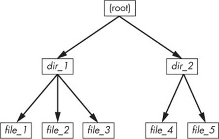
Figure 4-4. User-level representation of a filesystem
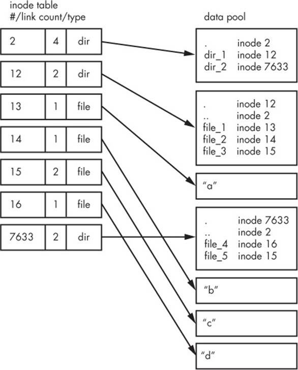
Figure 4-5. Inode structure of the filesystem shown in Figure 4-4
How do we make sense of this? For any ext2/3/4 filesystem, you start at inode number 2—the root inode. From the inode table in Figure 4-5, you can see that this is a directory inode (dir), so you can follow the arrow over to the data pool, where you see the contents of the root directory: two entries named dir_1 and dir_2 corresponding to inodes 12 and 7633, respectively. To explore those entries, go back to the inode table and look at either of those inodes.
To examine dir_1/file_2 in this filesystem, the kernel does the following:
1. Determines the path’s components: a directory named dir_1, followed by a component named file_2.
2. Follows the root inode to its directory data.
3. Finds the name dir_1 in inode 2’s directory data, which points to inode number 12.
4. Looks up inode 12 in the inode table and verifies that it is a directory inode.
5. Follows inode 12’s data link to its directory information (the second box down in the data pool).
6. Locates the second component of the path (file_2) in inode 12’s directory data. This entry points to inode number 14.
7. Looks up inode 14 in the directory table. This is a file inode.
At this point, the kernel knows the properties of the file and can open it by following inode 14’s data link.
This system, of inodes pointing to directory data structures and directory data structures pointing to inodes, allows you to create the filesystem hierarchy that you’re used to. In addition, notice that the directory inodes contain entries for . (the current directory) and .. (the parent directory, except for the root directory). This makes it easy to get a point of reference and to navigate back down the directory structure.
4.5.1 Viewing Inode Details
To view the inode numbers for any directory, use the ls -i command. Here’s what you’d get at the root of this example. (For more detailed inode information, use the stat command.)
$ ls -i
12 dir_1 7633 dir_2
Now you’re probably wondering about the link count. You’ve already seen the link count in the output of the common ls -l command, but you likely ignored it. How does the link count relate to the files in Figure 4-5, in particular the “hard-linked” file_5? The link count field is the number of total directory entries (across all directories) that point to an inode. Most of the files have a link count of 1 because they occur only once in the directory entries. This is expected: Most of the time when you create a file, you create a new directory entry and a new inode to go with it. However, inode 15 occurs twice: First it’s created as dir_1/file_3, and then it’s linked to as dir_2/file_5. A hard link is just a manually created entry in a directory to an inode that already exists. The ln command (without the -s option) allows you to manually create new links.
This is also why removing a file is sometimes called unlinking. If you run rm dir_1/file_2, the kernel searches for an entry named file_2 in inode 12’s directory entries. Upon finding that file_2 corresponds to inode 14, the kernel removes the directory entry and then subtracts 1 from inode 14’s link count. As a result, inode 14’s link count will be 0, and the kernel will know that there are no longer any names linking to the inode. Therefore, it can now delete the inode and any data associated with it.
However, if you run rm dir_1/file_3, the end result is that the link count of inode 15 goes from 2 to 1 (because dir_2/file_5 still points there), and the kernel knows not to remove the inode.
Link counts work much the same for directories. Observe that inode 12’s link count is 2, because there are two inode links there: one for dir_1 in the directory entries for inode 2 and the second a self-reference (.) in its own directory entries. If you create a new directory dir_1/dir_3, the linkcount for inode 12 would go to 3 because the new directory would include a parent (..) entry that links back to inode 12, much as inode 12’s parent link points to inode 2.
There is one small exception. The root inode 2 has a link count of 4. However, Figure 4-5 shows only three directory entry links. The “fourth” link is in the filesystem’s superblock because the superblock tells you where to find the root inode.
Don’t be afraid to experiment on your system. Creating a directory structure and then using ls -i or stat to walk through the pieces is harmless. You don’t need to be root (unless you mount and create a new filesystem).
But there’s still one piece missing: When allocating data pool blocks for a new file, how does the filesystem know which blocks are in use and which are available? One of the most basic ways is with an additional management data structure called a block bitmap. In this scheme, the filesystem reserves a series of bytes, with each bit corresponding to one block in the data pool. A value of 0 means that the block is free, and a 1 means that it’s in use. Thus, allocating and deallocating blocks is a matter of flipping bits.
Problems in a filesystem arise when the inode table data doesn’t match the block allocation data or when the link counts are incorrect; this can happen when you don’t cleanly shut down a system. Therefore, when you check a filesystem, as described in 4.2.11 Checking and Repairing Filesystems, the fsck program walks through the inode table and directory structure to generate new link counts and a new block allocation map (such as the block bitmap), and then it compares the newly generated data with the filesystem on the disk. If there are mismatches, fsck must fix the link counts and determine what to do with any inodes and/or data that didn’t come up when it traversed the directory structure. Most fsck programs make these “orphans” new files in the filesystem’s lost+found directory.
4.5.2 Working with Filesystems in User Space
When working with files and directories in user space, you shouldn’t have to worry much about the implementation going on below them. You’re expected to access the contents of files and directories of a mounted file-system through kernel system calls. Curiously, though, you do have access to certain filesystem information that doesn’t seem to fit in user space—in particular, the stat() system call returns inode numbers and link counts.
When not maintaining a filesystem, do you have to worry about inode numbers and link counts? Generally, no. This stuff is accessible to user mode programs primarily for backward compatibility. Furthermore, not all filesystems available in Linux have these filesystem internals. The Virtual File System (VFS) interface layer ensures that system calls always return inode numbers and link counts, but those numbers may not necessarily mean anything.
You may not be able to perform traditional Unix filesystem operations on nontraditional filesystems. For example, you can’t use ln to create a hard link on a mounted VFAT filesystem because the directory entry structure is entirely different.
Fortunately, the system calls available to user space on Unix/Linux systems provide enough abstraction for painless file access—you don’t need to know anything about the underlying implementation in order to access files. In addition, filenames are flexible in format and mixed-case names are supported, making it easy to support other hierarchical-style filesystems.
Remember, specific filesystem support does not necessarily need to be in the kernel. In user-space filesystems, the kernel only needs to act as a conduit for system calls.
4.5.3 The Evolution of Filesystems
As you can see, even the simple filesystem just described has many different components to maintain. At the same time, the demands placed on filesystems continuously increase with new tasks, technology, and storage capacity. Today’s performance, data integrity, and security requirements are beyond the offerings of older filesystem implementations, so filesystem technology is constantly changing. We’ve already mentioned Btrfs as an example of a next-generation filesystem (see 4.2.1 Filesystem Types).
One example of how filesystems are changing is that new filesystems use separate data structures to represent directories and filenames, rather than the directory inodes described here. They reference data blocks differently. Also, filesystems that optimize for SSDs are still evolving. Continuous change in the development of filesystems is the norm, but keep in mind that the evolution of filesystems doesn’t change their purpose.
All materials on the site are licensed Creative Commons Attribution-Sharealike 3.0 Unported CC BY-SA 3.0 & GNU Free Documentation License (GFDL)
If you are the copyright holder of any material contained on our site and intend to remove it, please contact our site administrator for approval.
© 2016-2026 All site design rights belong to S.Y.A.