MICROSOFT BIG DATA SOLUTIONS (2014)

Part III. Storing and Managing Big Data

In This Part

· Chapter 4: HDFS, Hive, HBase, and HCatalog

· Chapter 5: Storing and Managing Data in HDFS

· Chapter 6: Adding Structure with Hive

· Chapter 7: Expanding Your Capability with HBase and HCatalog

Chapter 4. HDFS, Hive, HBase, and HCatalog

What You Will Learn in This Chapter

· Exploring HDFS

· Working with Hive

· Understanding HBase and HCatalog

One of the key pieces of the Hadoop big data platform is the file system. Functioning as the backbone, it is used to store and later retrieve your data, making it available to consumers for a multitude of tasks, including data processing.

Unlike the file system found on your desktop computer or laptop, where drives are typically measured in gigabytes, the Hadoop Distributed File System (HDFS) must be capable of storing files where each file can be of gigabyte or terabyte sizes. This presents a series of unique challenges that must be overcome.

This chapter discusses the HDFS, its architecture, and how it solves many of the hurdles, such as reliably storing your big data, efficient access, and other tasks like replicating data throughout your cluster. We will also look at Hive, HBase, and HCatalog, all platforms or tools available within the Hadoop ecosystem that help simplify the management and subsequent retrieval of data out of HDFS.

Exploring the Hadoop Distributed File System

Originally created as part of a web search engine project called Apache Nutch, HDFS is a distributed file system designed to run on a cluster of cost-effective commodity hardware. Although there are a number of distributed file systems in the marketplace, several notable characteristics make HDFS really stand out. These characteristics align with the overalls goals as defined by the HDFS team and are enumerated here:

· Fault tolerance: Instead of assuming that hardware failure is rare, HDFS assumes that failures are instead the norm. To this end, an HDFS instance consists of multiple machines or servers that each stores part of the data. Because the data is distributed, HDFS can quickly detect faults and failures and subsequently automatically and transparently recover.

· High throughput: Where most file systems strive for low-latency operations, HDFS is more focused on high throughput, even at the expense of latency. This characteristic means that HDFS can stream data to its clients to support analytical processing over large sets of data and favors batch over interactive operations. With forward-looking features like caching and tiered storage, it will no longer be the case that HDFS is not good for interactive operations.

· Support for large data sets: It's not uncommon for HDFS to contain files that range in size from several gigabytes all the way up to several terabytes and can include data sets in excess of tens of millions of files per instance (all accomplished by scaling on cost-effective commodity hardware).

· Write-once read-many (WORM) principle: This is one of the guiding principles of HDFS and is sometimes referred to as coherency. More simply put, data files in HDFS are written and when closed are never updated. This simplification enables the high level of throughput obtained by HDFS.

· Data locality: In a normal application scenario, a process requests data for a source; the data is then transferred from the source over a network to the requestor who can then process it. This time tested and proven process often works fine on smaller data sets. As the size of the data set grows, however, bottlenecks and hotspots begin to appear. Server resources and networks can quickly become overwhelmed as the whole process breaks down. HDFS overcomes this limitation by providing facilities or interfaces for applications to move the computation to the data, rather than moving the data to the computation.

As one of the more critical pieces of the Hadoop ecosystem, it's worth spending a little extra time to understand the HDFS architecture and how it enables the aforementioned capabilities.

Explaining the HDFS Architecture

Before discussing machine roles or nodes, let's look at the most fundamental concept within HDFS: the block. You may already be familiar with the block concept as it is carried over from the file system found on your own computer. Blocks, in this context, are how files are split up so that they can be written to your hard drive in whatever free space is available.

A lot of functional similarities exist between your file system blocks and the HDFS block. HDFS blocks split files, some which may be larger than any single drive, so that they can be distributed throughout the cluster and subsequently written to each node's disk. HDFS blocks are also much larger than those in use on your local file system, defaulting to an initial size of 64MB (but often being allocated much larger).

Within an HDFS cluster, two types or roles of machines or servers make up what is often referred to as the master/slave architecture. The first, called the NameNode, functions as the master or controller for the entire cluster. It's responsible for maintaining all the HDFS metadata and drives the entire file system namespace operation. There can be only one single NameNode per cluster, and if it is lost or fails, all the data in the HDFS cluster is gone.

The second type of role within an HDFS cluster is the DataNode. And although there is only one NameNode, there are usually many DataNodes. These nodes primarily interact with HDFS clients by taking on the responsibility to read and write or store data or data blocks. This makes scaling in your cluster easy, as you simply add additional DataNodes to your cluster to increase capacity. The DataNode is also responsible for replicating data out when instructed to do so by the NameNode (more on HDFS replication shortly).

HDFS Read and Write Operations

To get a better understanding of how these parts or pieces fit together, Figure 4.1 and Figure 4.2 illustrate how a client reads from and writes to an HDFS cluster.

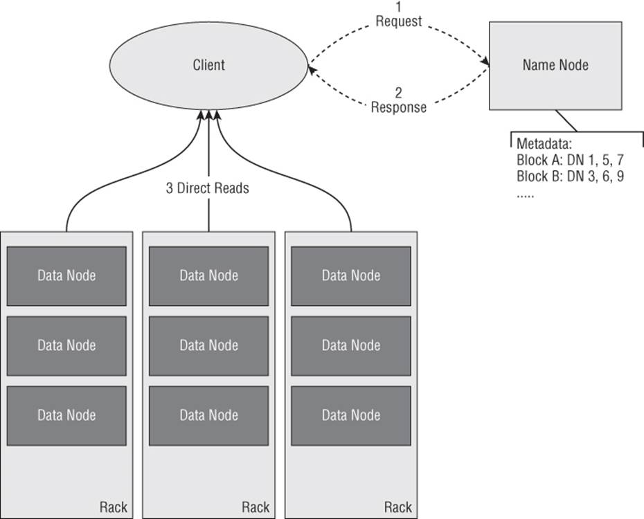
Figure 4.1 HDFS read operation

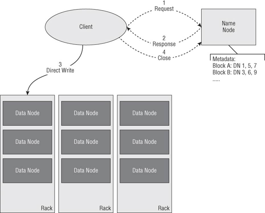
Figure 4.2 HDFS write operation

When a client needs to read a data set from HDFS (see Figure 4.1), it must first contact the NameNode. The NameNode contains all the metadata associated with the data set or file, including its blocks and all the block storage locations. The NameNode passes this metadata or information back to the client. The client then subsequently requests the data directly for each DataNode.

The pattern of this interaction is important. Although the NameNode acts as a gatekeeper, after the metadata is provided to the client, it gets out of the way and allows the client to interact directly with the DataNode. This provides the foundation for the extremely high level of throughput in HDFS.

Much like the read operation, an HDFS write-operation begins with the NameNode (see Figure 4.2). First, the client requests that the NameNode create a new empty file with no blocks associated with it. Next, the client streams data directly to the DataNode using an internal queue to reliably manage the process of sending and acknowledging the data.

Throughout the streaming process, as new blocks are allocated, the NameNode is updated. After the client has completed the write operation, it closes out the process with the NameNode. The NameNode only verifies that the minimum set of replicas have been created before returning successfully.

NOTE

Throughout this process, any write failures are handled silently and transparently to the client. If a node fails during the write or during the replicate process, it will be reattempted on an alternative node automatically.

Replication

Replication provides for fault tolerance within HDFS and occurs as part of each write or whenever the NameNode detects a DataNode failure. Out of the box, the default HDFS replication factor is three (controlled by the dfs.replication property), meaning that each block is written to three different nodes. Figure 4.3 elaborates on the previous write operation example to illustrate how replication occurs.

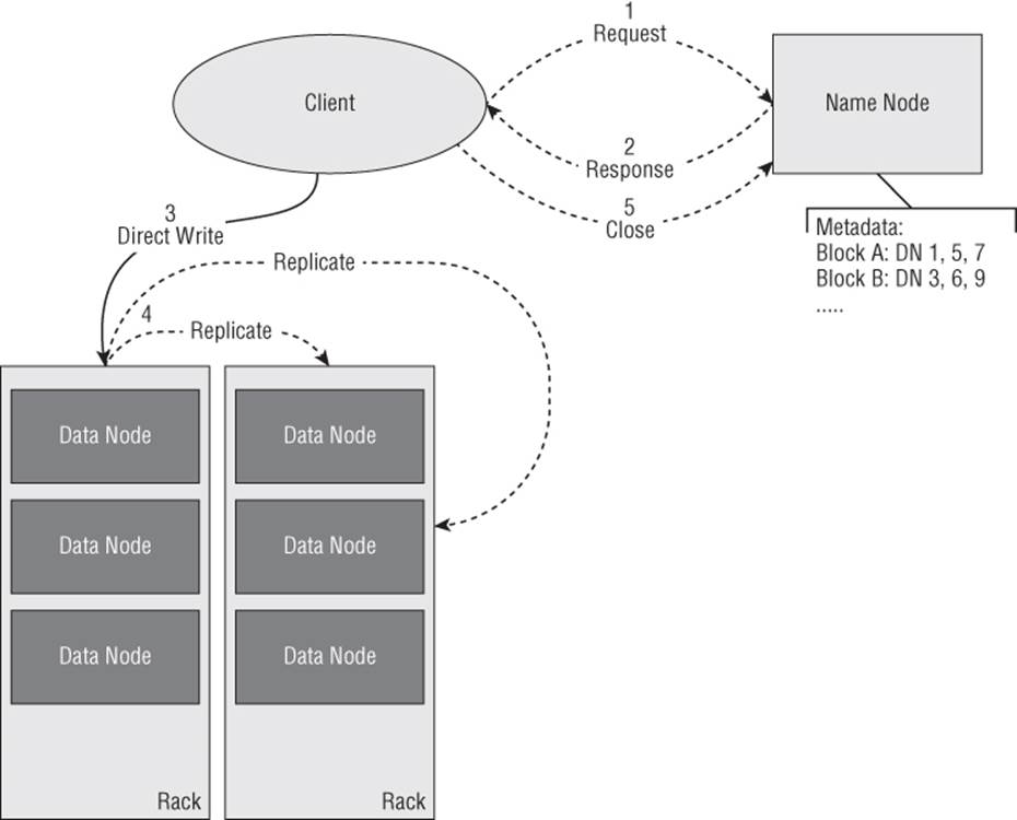
Figure 4.3 HDFS replication

During the course of the write the NameNode controls where replicated blocks are created and HDFS will create a minimum number of replicated blocks before the write is considered successful. Selecting the location for replicas is important for both fault tolerance and availability. HDFS is server, rack, and data center aware and is sophisticated in placement of replicated data so that maximum fault tolerance is achieved.

NOTE

The dfs.replication.min property controls the minimum number of replicas that must be created. If there is a difference between the dfs.replication and dfs.replication.min properties, the additional replicas are created asynchronously.

Interacting with HDFS

Because HDFS is built on top of the Java platform, the majority of integration and interaction options all require some level of Java development. Although these options, which range from the HDFS application programming interface (API) to Apache Thrift, are important (particularly if you are writing native client interactions), this chapter introduces only two of those most commonly used on the Microsoft platform: the HDFS command shell and WebHDFS. This is not intended to discount the other available options; instead, it is intended to help you get your feet wet as you get started with HDFS.

Hadoop File System (FS) Shell

Whether you realized it or not, you've already seen the HDFS command shell in action. As you worked through the Hortonworks Data Platform On-Premise introduction, the commands used to both upload and retrieve data from HDFS were all handled by the File System (FS) shell.

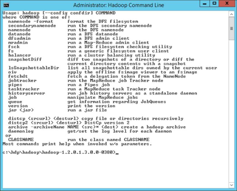
Figure 4.4 HDFS shell

The FS shell is actually part of Hadoop and uses commands that primarily align with UNIX commands. The FS shell commands all take the following format:

hadoop fs -<CMD> <ARGS>

The CMD is a specific file system command, and ARGS are the arguments needed to execute the command. The FS shell commands all use uniform resource indicators (URIs) in the format of [schema]://[authority]/[path]. For HDFS, these paths look like this:hdfs://node/mydata. The hdfs:// prefix is optional and is often left off for simplicity.

Table 4.1 lists some of the most common commands and shows usage examples.

Table 4.1 Hadoop File System Shell Commands

WebHDFS

The Hadoop FS shell is simple to get started with and straightforward to use for data management operations, but it has one potential weakness: The shell commands are just that, shell commands. Therefore, they require access to a machine with Hadoop installed to execute the commands.

NOTE

WebHDFS is just one of the many approaches for working with HDFS. There are advantages and disadvantages associated with each option.

An alternative to this approach, and one that overcomes this limitation, is WebHDFS. WebHDFS is an HTTP-based REST (Representational State Transfer) API that fully implements the same file system commands found in the FS shell.

Accessing this API is accomplished by embedding commands into HTTP URL requests and taking advantage of the standard HTTP operations (GET, POST, PUT, DELETE). To better illustrate, consider the following example to open a file via WebHDFS:

http://<HOST>:<PORT>/webhdfs/v1/<PATH>?op=OPEN

To deconstruct this URL for better understanding, note the following:

· The <HOST> and <PORT> arguments point to the location of the NameNode.

· The <PATH> argument is the file being requested.

· The op querystring parameter passes in the file system operation.

An HTTP GET request is issued using the example URL. After the path and location metadata is queried from the NameNode, an HTTP 307 temporary redirect is returned to the requestor, as shown here:

HTTP/1.1 307 TEMPORARY_REDIRECT

Location: http://<DATANODE>:<PORT>/webhdfs/v1/<PATH>?op=OPEN…

Content-Length: 0

The redirect contains the actual path to the DataNode that hosts the data file or block. The client can then follow the redirect to stream the data directly from the source.

As previously mentioned, the WebHDFS offers a complete implementation of the FS shell commands, Table 4.2 list some of the file system commands and their WebHDFS equivalents.

Table 4.2 WebHDFS Access Commands

Now that you are familiar with the basic concepts behind HDFS, let's look at some of the other functionality that is built on top of HDFS.

Exploring Hive: The Hadoop Data Warehouse Platform

Within the Hadoop ecosystem, HDFS can load and store massive quantities of data in an efficient and reliable manner. It can also serve that same data back up to client applications, such as MapReduce jobs, for processing and data analysis.

Although this is a productive and workable paradigm with a developer's background, it doesn't do much for an analyst or data scientist trying to sort through potentially large sets of data, as was the case with Facebook.

Hive, often considered the Hadoop data warehouse platform, got its start at Facebook as their analyst struggled to deal with the massive quantities of data produced by the social network. Requiring analysts to learn and write MapReduce jobs was neither productive nor practical.

Instead, Facebook developed a data warehouse-like layer of abstraction that would be based on tables. The tables function merely as metadata, and the table schema is projected onto the data, instead of actually moving potentially massive sets of data. This new capability allowed their analyst to use a SQL-like language called Hive Query Language (HQL) to query massive data sets stored with HDFS and to perform both simple and sophisticated summarizations and data analysis.

Designing, Building, and Loading Tables

If you are familiar with basic T-SQL data definition language (DDL) commands, you already have a good head start in working with Hive tables. To declare a Hive table, a CREATE statement is issued similar to those used to create tables in a SQL Server database. The following example creates a simple table using primitive types that are commonly found elsewhere:

CREATE EXTERNAL TABLE iislog (

date STRING,

time STRING,

username STRING,

ip STRING,

port INT,

method STRING,

uristem STRING,

uriquery STRING,

timetaken INT,

useragent STRING,

referrer STRING

)

ROW FORMAT DELIMITED FIELDS TERMINATED BY ',';

Two important distinctions need to be pointed out with regard to the preceding example. First, note the EXTERNAL keyword. This keyword tells Hive that for this table it only owns the table metadata and not the underlying data. The opposite of this keyword (and the default value) is INTERNAL, which gives Hive control of both the metadata and the underlying data.

The difference between these two options is most evident when the table is dropped using the DROP TABLE command. Because Hive does not own the data for an EXTERNAL table, only the metadata is removed, and the data continues to live on. For an INTERNAL table, both the table metadata and data are deleted.

The second distinction in the CREATE statement is found on the final line of the command: ROW FORMAT DELIMITED FIELDS TERMINATED BY ','. This command instructs Hive to read the underlying data file and split the columns or fields using a comma delimiter. This is indicative that instead of storing data in an actual table structure, the data continues to live in its original file format.

At this point, in this example, although we have defined a table schema, no data has been explicitly loaded. To load data after the table is created, you could use the following command to log all of your IIS web server log files that exist in the logs directory:

load data inpath '/logs'

overwrite into table iislog;

This demonstration only scratches the surface of the capabilities in Hive. Hive supports a robust set of features, including complex data types (maps, structs, and arrays), partitioning, views, and indexes. These features are beyond the scope of this book, but they certainly warrant further exploration if you intend to use this technology.

Querying Data

Like the process used previously to create a Hive table, HQL can be subsequently used to query data out for the purposes of summarization or analysis. The syntax, as you might expect, is almost identical to that use to query a SQL Server database. Don't be fooled, though. Although the interface looks a lot like SQL, behind the scenes Hive does quite a bit of heavy lifting to optimize and convert the SQL-like syntax to one or more MapReduce jobs that is used to satisfy the query:

SELECT *

FROM iislog;

This simple query, much like its counterparts in the SQL world, simply returns all rows found in the iislog table. Although this is not a sophisticated query, the HQL supports both basic operations such as sorts and joins to more sophisticated operations, including group by, unions, and even user-defined functions. The following example is a common example of a group by query to count the number of times each URI occurs in the web server logs:

SELECT uristem, COUNT(*)

FROM iislog

GROUP BY (uristem);

Configuring the Hive ODBC Driver

A wealth of third-party tools, such as Microsoft Excel, provide advanced analytic features, visualizations, and toolsets. These tools are often a critical part of a data analyst's day-to-day job, which make the Hive Open Database Connectivity (ODBC) driver one of the most important pieces of Hive. You can download the Hive ODBC driver from http://www.microsoft.com/en-us/download/details.aspx?id=40886. It allows any ODBC-compliant application to easily tap into and integrate with your big data store.

Configuring the Hive ODBC driver (see Figure 4.5) is handled using the ODBC Data Sources configuration tool built in to the Microsoft Windows operating system. After configuration is complete, Hive tables can be accessed directly from not only analytics tools such as Microsoft Excel but also from other ODBC-compliant tools such as SQL Server Integration Services (SSIS).

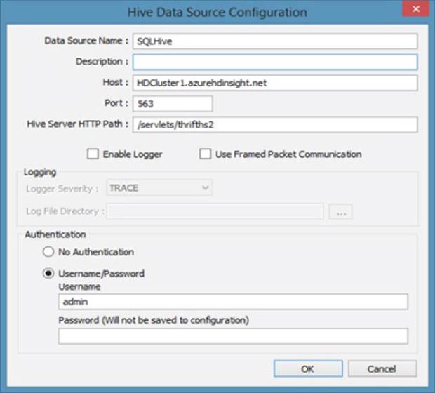
Figure 4.5 Hive ODBC configuration

Exploring HCatalog: HDFS Table and Metadata Management

In the previous examples, the source use for our Hive table is an HDFS path. This is common within the Hadoop ecosystem. While referencing these paths directly works fine and is perfectly acceptable in many scenarios, what it does is bind your Hive table or Pig job to a specific data layout within HDFS.

If this data layout were to change during an activity like data maintenance or simply because the size of the data outgrew the initial HDFS organizational structure, your script or job would be broken. This would require you to revisit every script or job that referenced this data, which in large systems could be potentially unpleasant.

This scenario is just one of the reasons the Apache HCatalog project was created. HCatalog started as an abstraction of the Hive metadata management functionality (currently is part of the larger Apache Hive project) and is intended to allow for shared metadata across the Hadoop ecosystem.

Table definitions and even data type mappings can be created and shared, so users can work with data stored in HDFS without worrying about the underlying details such as where or how the data is stored. HCatalog currently works with MapReduce, Hive, and of course, Pig; and as an abstraction of the Hive platform, the syntax for creating tables is identical, except that we have to specify the data location during creation of the table:

CREATE EXTERNAL TABLE iislog (

date STRING,

time STRING,

username STRING,

ip STRING,

port INT,

method STRING,

uristem STRING,

uriquery STRING,

timetaken INT,

useragent STRING,

referrer STRING

)

ROW FORMAT DELIMITED FIELDS TERMINATED BY ','

STORED AS TEXTFILE

LOCATION '/data/logs';

Our iislog table can now be referenced directly one or more times in Hive by simply using the table name, as seen previously. Because HCatalog is integrated across platforms, the same table can also be referenced in a Pig job.

Let's look first at an example of a simple Pig Latin script that references the data location directly and includes the column schema definition:

A = load '/data/logs' using PigStorage() as (date:chararray,

time:chararray, username:chararray, ip:chararray,

port:int, method:chararray, uristem:chararray,

uriquery:chararray, timetaken:int,

useragent:chararry, referrer:chararray);

You can compare and contrast the code samples to see how HCatalog simplifies the process by removing both the data storage location and schema from the script:

A = load 'iislog' using HCatLoader();

In this example, if the underlying data structure were to change and the location of the logs were moved from the /data/logs path to /archive/2013/weblogs, the HCatalog metadata could be updated using the ALTER statement. This allows all the Hive script, MapReduce, and Pig jobs that are using the HCatalog to continue to run without modification:

ALTER EXTERNAL TABLE iislog

LOCATION '/archive/2013/weblogs ';

Together, these features allow Hive to look and act like a database or data warehouse over your big data. In the next section, we will explore a different implementation that provides a No-SQL database on top of HDFS.

Exploring HBase: An HDFS Column-oriented Database

So far, all the techniques presented in this chapter have a similar use case. They are all efficient at simplifying access to your big data, but they have all largely been focused on batch-centric operations and are mostly inappropriate for interactive or real-time data access purposes. Apache HBase fills the gap in this space and is a NoSQL database built on top of Hadoop and HDFS that provides real-time, random read/write access to your big data.

The Apache HBase project is actually a clone modeled after the Google BigTable project defined by Chang et al. (2006) in the paper “BigTable: A Distributed Storage System for Structured Data.” You can review the whole paper athttp://research.google.com/archive/bigtable.html, but a summary or overview of columnar databases in general will suffice to get you going.

NoSQL Database Types

The term NoSQL often refers to nonrelational databases. There are four common types of NoSQL databases:

· Key/value: The simplest of the NoSQL databases, key/value databases are essentially hash sets that consist of a unique key and a value that is often represented as a schema-less blob.

· Document: Similar to key/value databases, document databases contain structured documents (such as XML, JSON, or even HTML) in place of the schema-less blob. These systems usually provide functionality to search within the stored documents.

· Columnar: Instead of storing data in a row/column approach, data in a columnar database is organized by column families which are groups of related columns, as discussed in more detail in the following section.

· Graph: The graph database consists of entities and edges, which represent relationships between nodes. The relationships between nodes can contain properties, which include items like direction of the relationship. This type of NoSQL database is commonly used to traverse organization or social network data.

Columnar Databases

If you are familiar with relational database systems, you are without a doubt familiar with the traditional column and row layout used. To demonstrate the differences, let's look at a concrete example.

Consider the entity-relationship diagram (ERD) shown in Figure 4.6. It uses a pretty common approach to model a one-to-many relationship between customers and addresses. Like you've probably been taught throughout the years, it is highly normalized and follows good relational database design principles. Figure 4.7 illustrates a populated customer and address model based on the ERD found in Figure 4.6.

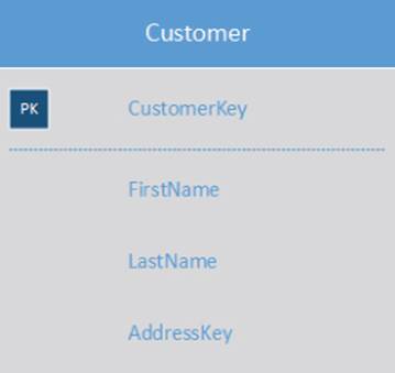
Figure 4.6 Entity-relationship diagram

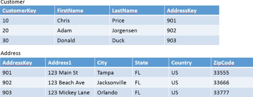
Figure 4.7 Traditional database structure

Relational designs and databases do not easily scale and cannot typically handle the volumes, variety, and velocity associated with big data environments. This is where NoSQL databases such as HBase were designed to excel, yet they represent a very different way of thinking about and ultimately storing your data.

HBase is a columnar database, which means that instead of being organized by rows and columns, it is organized by column families, which are sets of related columns. Restructuring the data presented in Figure 4.7 using the columnar approach results in a layout that although similar is actually very different (see Figure 4.8).

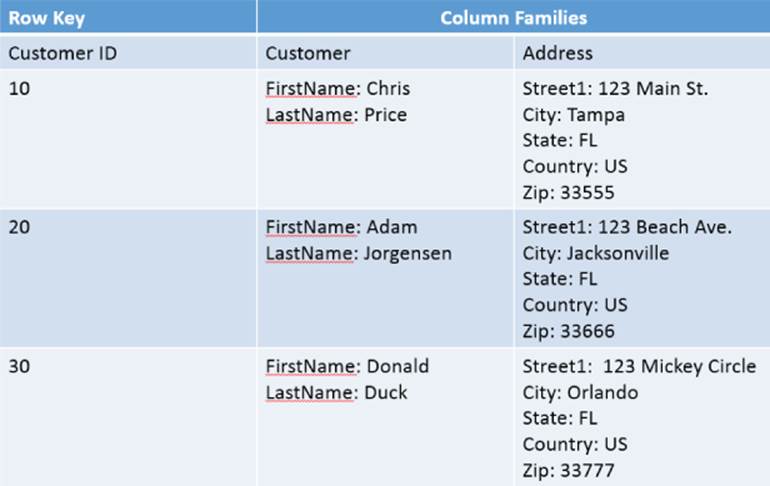
Figure 4.8 Columnar database structure

The columnar layout has many advantages over a relational model in the context of handling big data, including the following:

· Can handle very large (even massive) quantities of data through a process known as sharding

· Allows flexible data formats that can vary from row to row

· Typically scales linearly

For a more thorough discussion on columnar database capabilities and HBase in general, check out the HBase website at http://hbase.apache.org/.

Defining and Populating an HBase Table

HBase is installed and configured for you as part of the Hortonworks Data Platform. You can work with HBase directly from the HBase command shell.

To define a table, you specify a table name and the column family or families. In the following example, a basic customer table with a single column family for addresses is created:

create 'customer', 'address'

Take note that no schema or columns were defined for the actual table or the column family. This is intentional because the actual columns contained within an address could vary.

At this point, you may be questioning why this is a desirable behavior. There are actually a number of use cases; the easiest involves international addresses. Consider a U.S. address that has parts like address1, address2, city, state, and ZIP code. Other regions and countries do not necessarily follow this same format, so the flexibility is desirable in this scenario.

Now, let's take a quick look at how we put data into our customer table using the put statement:

put 'customer', 'row01', 'address:street', '123 Main St.'

put 'customer', 'row01', 'address:city', 'Tampa'

put 'customer', 'row01', 'address:state', 'Florida'

put 'customer', 'row01', 'address:country', 'United States of America'

put 'customer', 'row01', 'address:zip', '34637'

The format of this command specifies the table name (customer), the row identifier (row01), the column family and column name (address:[xxx]), and finally the value. When the commands complete, the data is available for query operations.

NOTE

To drop an HBase table, you must first disable it, and then drop it. The syntax to perform this operation is as follows:

disable 'customer'

drop 'customer'

Using Query Operations

To retrieve the data from the HBase table you just created, there are two fundamental methods available through the HBase shell. The scan command indiscriminately reads the entire contents of your table and dumps it to the console window:

scan 'customer'

For small tables, this command is useful for verifying that the table is configured and set up correct. When working with a larger table, it is preferable to use a more targeted query. The get command accomplishes this:

get 'customer' 'row01'

To use the get command, you specify the table name (customer) followed by the row key (row01). This returns all the column families and associated columns for the given key.

A more thorough discussion of HBase is beyond the scope of this book, but it's worth noting that HBase supports updating and deleting rows. There are also robust and fully functional Java and REST APIs available for integrating HBase outside the Hadoop ecosystem.

Summary

Hadoop offers a number of different methods or options for both storing and retrieving your data for processing and analytical purposes. HDFS is the Hadoop file system that provides a reliable and scalable platform for hosting your data. HDFS is also well suited to serve your data to other tools within the Hadoop ecosystem, like MapReduce and even Pig jobs.

Hive, the Hadoop Data Warehousing platform, is also built on top of HDFS. Using the HQL, you can easily project a schema onto your data and then use SQL-like syntax to summarize and analyze your data.

To build more robust solutions, you can implement HCatalog to abstract the details of how your big data is stored. HCatalog provides table and metadata management that is built on top of Hive and integrates well into the Hadoop stack of tools.

Finally, when it becomes necessary to provide real-time, random read/write capabilities to your data, the Apache HBase project provides a columnar NoSQL database implementation also built on top of HDFS. Together, these tools and platforms give you many different options to tackle a number of different use cases in the diverse big data space.