MICROSOFT BIG DATA SOLUTIONS (2014)

Part III. Storing and Managing Big Data

Chapter 6. Adding Structure with Hive

What You Will Learn in This Chapter

· Learning How Hive Provides Value in a Hadoop Environment

· Comparing Hive to a Relational Database

· Working With Data in Hive

· Understanding Advanced Options in Hive

This chapter discusses how you can use Hive with Hadoop to get more value out of your big data initiatives. Hive is a component of all major Hadoop distributions, and it is used extensively to provide SQL-like functionality from a Hadoop installation. For example, Hive is often used to enable common data warehouse scenarios on top of data stored in Hadoop. An example of this would be retrieving a summary of sales by store, and by department. Using MapReduce to prepare and produce these results would take multiple lines of Java code. By using Hive, you can write a familiar SQL query to get the same results:

SELECT Store, Department, SUM(SalesAmount)

FROM StoreSales

GROUP BY Store, Department

If you are familiar with SQL Server, or other relational databases, portions of Hive will seem very familiar. Other aspects of Hive, however, may feel very different or restrictive compared to a relational database. It's important to remember that Hive attempts to bridge some of the gap between Hadoop Distributed File System (HDFS) data store and the relational world, while providing some of the benefits of both technologies. By keeping that perspective, you'll find it easier to understand how and why Hive functions as it does.

Hive is not a full relational database, and limitations apply to the relational database management system (RDBMS) functionality it supports. The differences that are most likely to impact someone coming from a relational perspective are covered in this chapter. Although complete coverage of the administration and configuration of Hive is beyond the scope for this chapter, the discussion here does include basic commands for creating tables and working with data in Hive.

Understanding Hive's Purpose and Role

Hadoop was developed to handle big data. It does an admirable job of this; but in creating a new platform to solve this problem, it introduced a new challenge: people had to learn a new and different way to work with their data. Instead of using Structured Query Language (SQL) to retrieve and transform data, they had to use Java and MapReduce. Not only did this mean that data professionals had to learn a new skillset, but also that the SQL query tools that IT workers and business users traditionally used to access data didn't work against Hadoop.

Hive was created to address these needs and make it easier for people and tools to work with Hadoop data. It does that by acting as an interpreter for Hadoop; you give Hive instructions in Hive Query Language (HQL), which is a language that looks very much like SQL, and Hive translates that HQL into MapReduce jobs. This opens up Hadoop data to tools and users that understand SQL.

In addition to acting as a translator, Hive also answers another common challenge with data in Hadoop. Files stored in Hadoop do not have to share a common data format. They can be text files delimited by commas, control characters, or any of a wide variety of characters. It's not even necessary that they be delimited text files. They can be files that use binary format, XML, or any of a combination of different formats. Hive enables you to deliver the data to users in a way that adheres to a defined schema or format.

Hive addresses these issues by providing a layer on top of Hadoop data that resembles a traditional relational database. In particular, Hive is designed to support the common operations for data warehousing scenarios.

NOTE

Although Hive looks like a relational database, with tables, columns, indexes, and so on, and much of the terminology is the same, it is not a relational database. Hive does not enable referential integrity, it does not enable transactions, and it does not grant ACID (atomicity, consistency, isolation, and durability) properties to Hadoop data stores.

Providing Structure for Unstructured Data

Users and the tools they use for querying data warehouses generally expect tabular, well-structured data. They expect the data to be delivered in a row/column format, and they expect consistency in the data values returned. Take the example of a user requesting a data set containing all the sales transactions for yesterday. Imagine the user's reaction if some rows in the data set contained 10 columns, some contained 8 columns, and some contained 15. The user would also be very surprised to find that the unit cost column in the data set contained valid numeric values on some rows, and on others it might contain alpha characters.

Because Hadoop data stores don't enforce a particular schema, this is a very real scenario when querying Hadoop. Hive helps with this scenario by enabling you to specify a schema of columns and their types for the information. Then, when the data is queried through Hive, it ensures that the results conform to the expected schema.

These schemas are declared by creating a table. The actual table data is stored as files in the Hadoop file system. When you request data from the table, Hive translates that request to read the appropriate files from the Hadoop file system and returns the data in a format that matches the table definition provided.

The table definitions are stored in the Hive metadata store, or metastore. By default, the metastore is an embedded Derby database. This metastore is a relational database that captures the table metadata (the name of the table, the columns and data types it contains, and the format that the underlying files are expected to be in).

NOTE

In a default Hive setup, the Derby database used for the metastore may be configured for single-user access. If you are just testing Hive or running a local instance for development, this may be fine. However, for Hive implementation in a production environment, you will want to upgrade the metastore to a multiple-user setup using a more robust database. One of the more common databases used for this is MySQL. However, the metastore can be any Java Database Connectivity (JDBC)-compliant database. If you are using the Hortonworks' HDP 1.3 Windows distribution, SQL Server can be used as a supported metastore.

Hive v0.11 also includes HiveServer2. This version of Hive improves support for multi-user concurrency and supports additional authentication methods, while providing the same experience as the standard Hive server. Again, for a production environment, HiveServer2 may be a better fit. The examples used in this chapter run against Hive Server and HiveServer2.

Another area of difference between Hive and many relational databases is its support for different data types. Due to the unstructured data that it must support, it defines a number of data types that you won't find in a traditional relational database.

Hive Data Types

Table 6.1 lists the data types supported by Hive. Many of these data types have equivalent values in SQL Server, but a few are unique to Hive. Even for the data types that appear familiar, it is important to remember that Hive is coded as a Java application, and so these data types are implemented in Java. Their behavior will match the behavior from a Java application that uses the same data type. One immediate difference you will notice is that STRING types do not have a defined length. This is normal for Java and other programming languages, but is not typical for relational databases.

NOTE

DATE types are new for Hive 0.12. The Hortonworks Data Platform (HDP) 1.3 release is built using Hive 0.11, so this data type cannot be used with it yet.

Table 6.1 Hive Data Types

The types that are unique to Hive are MAP, ARRAY, and STRUCT. These types are supported in Hive so that it can better work with the denormalized data that is often found in Hadoop data stores. Relational database tables are typically normalized; that is, a row holds only one value for a given column. In Hadoop, though, it is not uncommon to find data where many values are stored in a row for a “column.” This denormalization of the data makes it easier and faster to write the data, but makes it more challenging to retrieve it in a tabular format.

Hive addresses this with the MAP, ARRAY, and STRUCT types, which let a developer flatten out the denormalized data into a multicolumn structure. The details of querying this denormalized data are discussed later in this chapter. For now, we will review the data types that support these structures.

A STRUCT is a column that contains multiple defined fields. Each field can have its own data type. This is comparable to structs in most programming languages. In Hive, you can declare a STRUCT for a full name using the following syntax:

STRUCT <FirstName:string, MiddleName:string, LastName:string>

To access the individual fields of the STRUCT type, use the column name followed by a period and the name of the field:

FullName.FirstName

An ARRAY is a column that contains an ordered sequence of values. All the values must be of the same type:

ARRAY<STRING>

Because it is ordered, the individual values can be accessed by their index. As with Java and .NET languages, ARRAY types use a zero-based index, so you use an index of 0 to access the first element, and an index of 2 to access the third element. If the preceding Full Name column were declared as an ARRAY, with first name in the first position, middle name in the second position, and last name in the third position, you would access the first name with index 0 and last name with index 2:

FullName[0], FullName[2]

A MAP column is a collection of key/value pairs, where both the key and values have data types. The key and value do not have to use the same data type. A MAP for Full Name might be declared using the following syntax:

MAP<string, string>

In the Full Name case, you would populate the MAP column with the following key/value pairs:

'FirstName', 'John'

'MiddleName', 'Doe'

'LastName', 'Smith'

You can access MAP column elements using the same syntax as you use with an ARRAY, except that you use the key value instead of the position as the index. Accessing the first and last names would be done with this syntax:

FullName['FirstName'], FullName['LastName']

After looking at the possible data types, you may be wondering how these are stored in Hive. The next section covers the file formats that can be used to store the data.

File Formats

Hive uses Hadoop as the underlying data store. Because the actual data is stored in Hadoop, it can be in a wide variety of formats. As discussed in Chapter 5, “Storing and Managing Data in HDFS,” Hadoop stores files and doesn't impose any restrictions in the content or format of those files. Hive offers enough flexibility that you can work with almost any file format, but some formats require significantly more effort.

The simplest files to work with in Hive are text files, and this is the default format Hive expects for files. These text files are normally delimited by specific characters. Common formats in business settings are comma-separated value files or tab-separated value files. However, the drawback of these formats is that commas and tabs often appear in real data; that is, they are embedded inside other text, and not intended as delimiters in all instances. For that reason, Hive by default uses control characters as delimiters, which are less likely to appear in real data. Table 6.2 describes these default delimiters.

NOTE

The default delimiters can be overridden when the table is created. This is useful when you are dealing with text files that use different delimiters, but are still formatted in a very similar way. The options for that are shown in the section “Creating Tables” in this chapter.

Table 6.2 Hive Default Delimiters for Text Files

What if one of the many text files that is accessed through a Hive table uses a different value as a column delimiter? In that case, Hive won't be able to parse the file accurately. The exact results will vary depending on exactly how the text file is formatted, and how the Hive table was configured. However, it's likely that Hive will find less than the expected number of columns in the text file. In this case, it will fill in the columns it finds values for, and then output null values for any “missing” columns.

The same thing will happen if the data values in the files don't match the data type defined on the Hive table. If a file contains alphanumeric characters where Hive is expecting only numeric values, it will return null values. This enables Hive to be resilient to data quality issues with the files stored in Hadoop.

Some data, however, isn't stored as text. Binary file formats can be faster and more efficient than text formats, as the data takes less space in the files. If the data is stored in a smaller number of bytes, more of it can be read from the disk in a single-read operation, and more of it can fit in memory. This can improve performance, particularly in a big data system.

Unlike a text file, though, you can't open a binary file in your favorite text editor and understand the data. Other applications can't understand the data either, unless they have been built specifically to understand the format. In some cases, though, the improved performance can offset the lack of portability of the binary file formats.

Hive supports several binary formats natively for files. One option is the Sequence File format. Sequence files consist of binary encoded key/value pairs. This is a standard file format for Hadoop, so it will be usable by many other tools in the Hadoop ecosystem.

Another option is the RCFile format. RCFile uses a columnar storage approach, rather than the row-based approach familiar to users of relational systems. In the columnar approach, the values in a column are compressed so that only the distinct values for the column need to be stored, rather than the repeated values for each row. This can help compress the data a great deal, particularly if the column values are repeated for many rows. RCFiles are readable through Hive, but not from most other Hadoop tools.

A variation on the RCFile is the Optimized Record Columnar File format (ORCFile). This format includes additional metadata in the file system, which can vastly speed up the querying of Hive data. This was released as part of Hive 0.11.

NOTE

Compression is an option for your Hadoop data, and Hive can decompress the data as needed for processing. Hive and Hadoop have native support for compressing and decompressing files on demand using a variety of compression types, including common formats like Zip compression. This can be an alternative that allows to you get the benefits of smaller data formats while still keeping the data in a text format.

If the data is in a binary or text format that Hive doesn't understand, custom logic can be developed to support it. The next section discusses how these can be implemented.

Custom File and Record Formats

Hive leverages Hadoop's ability to use custom logic for processing files. A full discussion of the implementation of custom logic for this is beyond the scope of this chapter, but this section does cover the basics.

First, you want to understand that Hive (and Hadoop in general) makes a distinction between the file format and the record format. The file format determines how records are stored in the file, and the record format determines how individual fields are extracted from each record.

By default, Hive uses the TEXTFILE format for the file format. You can override this for each Hive table by specifying a custom input format and a custom output format. The input format controls how records are written to the file, and the output format controls how the record is read from the file. If the record format of the file doesn't match one of the natively supported formats, you must provide an implementation of both the input format and output format, or Hive will not be able to use the file. Implementing the custom input and output formats is usually done in Java, although Microsoft is providing support for .NET-based implementations as well.

The record format is the next aspect to consider. As discussed already, the default record format is a text with delimiters between fields. If the record format requires custom processing, you must provide a reference to a serializer/deserializer (or SerDe). SerDes implements the logic for serializing the fields in a record to a specific record format and for deserializing that record format back to the individual fields.

Hive includes a couple of standard SerDes. The delimited record format is the default SerDe, and it can be customized to use different delimiters, in the event that a file uses a record format with nonstandard delimiters.

One of the other included SerDes handles regular expressions. The RegexSerde is useful when processing web logs and other text files where the format can vary but values can be extracted using pattern matching.

Third-Party SerDes

Third-party SerDes are available for Hive as well. Examples include CSVSerde (https://github.com/ogrodnek/csv-serde), which handles CSV files with embedded quotes and delimiters, and a JSON SerDe (https://github.com/cloudera/cdh-twitter-example/blob/master/hive-serdes/src/main/java/com/cloudera/hive/serde/JSONSerDe.java), which will parse records stored as JSON objects.

Hive has robust support for both standard and complex data types, stored in a wide variety of formats. And as highlighted in the preceding section, if support for a particular file format is not included, it can be added via third-party add-ons or custom implementations. This works very well with the type of data that is often found in Hadoop data stores. By using Hive's ability to apply a tabular structure to the data, it makes it easier for users and tools to consume. But there is another component to making access much easier for existing tools, which is discussed next.

Enabling Data Access and Transformation

Traditional users of data warehouses expect to be able to query and transform the data. They use SQL for this. They run this SQL through applications that use common middleware software to provide a standard interface to the data. Most RDBMS systems implement support for one or more of these middleware interfaces. Open Database Connectivity (ODBC) is a common piece of software for this and has been around since the early 1990s. Other common interfaces include the following:

· ADO.NET (used by Microsoft .NET-based applications)

· OLE DB

· Java Database Connectivity (JDBC)

ODBC, being one of the original interfaces for this, is well supported by existing applications, and many of the other interfaces provide bridges for ODBC.

Hive provides several forms of connectivity to Hadoop data through Thrift. Thrift is a software framework that supports network service communication, including support for JDBC and ODBC connectivity. Because ODBC is broadly supported by query access tools, it makes it much easier for business users to access the data in Hadoop using their favorite analysis tools. Excel is one of the common tools used by end users for working with data, and it supports ODBC. (Using Excel with Hadoop is discussed further in Chapter 11, “Visualizing Big Data with Microsoft BI.”)

In addition to providing ODBC data access, Hive also acts as a translator for the SQL. As mentioned previously, many users and developers are familiar with writing SQL statements to query and transform data. Hive can take that SQL and translate it into MapReduce jobs. So, rather than the business users having to learn Java and MapReduce, or learn a new tool for querying data, they can leverage their existing knowledge and skills.

Hive manages this SQL translation by providing Hive Query Language (HQL). HQL provides support for common SQL language operations like SELECT for retrieving information and INSERT INTO to load data. Although HQL is not ANSI SQL compliant, it implements enough of the standard to be familiar to users who have experience working with RDBMS systems.

Differentiating Hive from Traditional RDBMS Systems

This chapter has discussed several of the ways that Hive emulates a relational database. It's also covered some of the ways in which it differs, including the data types and the storage of the data. Those topics are worth covering in a bit more depth because they do have significant impact on how Hive functions and what you should expect from it.

In a relational database like SQL Server, the database engine manages the data storage. That means when you insert data into a table in a relational database, the server takes that data, converts it into whatever format it chooses, and stores it in data structures that it manages and controls. At that point, the server becomes the gatekeeper of the data. To access the data again, you must request it from the relational database so that the server can retrieve it from the internal storage and return it to you. Other systems cannot access or change the data directly without going through the server.

Hive, however, uses Hadoop as its data storage system. Therefore, the data sits in HDFS and is accessible to anyone with access to the file system. This does make it easier to manage the data and add new information, but you must be aware that other processes can manipulate the data.

One of the primary differences between Hive and most relational systems is that data in Hive can only be selected, inserted, or deleted; there is no update capability. This is due to Hive using Hadoop file storage for its data. As noted in Chapter 8, “Effective Big Data ETL with SSIS, Pig, and Sqoop,” Hadoop is a write-once, read-many file system. If you need to change something in a file, you delete the original and write a new version of the file. Because Hive manages table data using Hadoop, the same constraints apply to Hive. There are also no row-based operations. Instead, everything is done in bulk mode.

Another key difference is that the data structure is defined up-front in traditional relational databases. The columns of a table, their data types, and any constraints on what the column can hold are set when the table is created. The database server enforces that any data written to the table conforms to the rules set up when the table was created. This is referred to as schema on write; the relational database server enforces the schema of the data when it is written to the table. If the data does not match the defined schema, it will not be inserted into the table.

Because Hive doesn't control the data and can't enforce that it is written in a specific format, it uses a different approach. It applies the schema when the data is read out of the data storage: schema on read. As mentioned, if the number of columns in the file is less than what is defined in Hive, null values are returned for the missing columns. If the data types don't match, null values are returned for those columns as well. The benefit of this is that Hive queries rarely fail due to bad data in the files. However, you do have to ensure that the data coming back is still meaningful and doesn't contain so many null values that it isn't useful.

Working with Hive

Like many Hadoop tools, Hive leverages a command-line interface (CLI) for interaction with the service. Other tools are available, such as the Hive Web Interface (HWI) and Beeswax, a user interface that is part of the Hue UI for working with Hadoop. For the examples in this chapter, though, the command line is used.

NOTE

Beeswax and Hue are not yet supported in HDInsight or the Hortonworks HDP 1.3 distribution, but it is under development. In the meantime, the CLI is the primary means of interacting directly with Hive.

You can launch the CLI by navigating to the Hive bin folder (c:\hdp\hadoop\hive-0.11.0.1.3.0.0-0380\bin in the Hortonworks HDP 1.3 distribution with the default setup). Once there, run the CLI by executing the hive.cmd application. After the CLI has been run, you'll notice that the prompt changes to hive (see Figure 6.1).

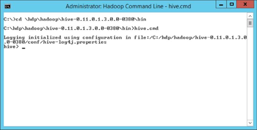
Figure 6.1 Hive CLI Interface

When executing Hive commands through the CLI, you must put a semicolon on each line of code that you want to execute. You can enter multiple lines, and the CLI will buffer them, until a semicolon is entered. At that point, the CLI executes all the proceeding commands.

A useful feature of the Hive CLI is the ability to run hadoop dfs commands without exiting. The Hive CLI uses an alias so that you can simply reference dfs directly, without the hadoop keyword, and it will execute the dfs command and return the results. For example, running the following code from the Hive prompt returns a recursive directory listing from the Hadoop file system:

dfs -lsr

The Hive CLI also supports basic autocomplete; that is, if you start typing a keyword or function and press the Tab key, it tries to complete the word. For example, if you type in cre and press Tab, it will complete it to create. If you press Tab on a new line, it prompts you if you want a list of all 427 possibilities. The CLI also maintains a history of previous commands entered. You can retrieve these values by pressing the up- and down-arrow keys. If you have a previously entered command selected, you can press the Enter key to run it again.

Creating and Querying Basic Tables

This section covers the basics of creating and organizing tables in Hive, as well as how to query them. If you are comfortable with SQL, you should find the commands familiar.

Creating Databases

Hive databases are essentially a way to organize tables. They are similar to the concept of a schema in SQL Server. In fact, Hive supports SCHEMA as a synonym for the DATABASE keyword. Databases are most often used to organize tables when there are multiple groups using the Hive server. When a database is created, Hive creates a folder in the Hadoop file system, by default using the same name as specified for the database, with.db appended to it. Any objects that are created using that database will be stored in the database's directory. If you don't specify a database when you create a table, it will be created in the default database.

To create a database, use the CREATE DATABASE command, followed by the name of the database:

CREATE DATABASE MsBigData;

NOTE

Many commands in Hive support IF EXISTS or IF NOT EXISTS clauses. Generally, you can use IF NOT EXISTS when creating objects, and IF EXISTS when removing them. These are used to check whether the target object is in the correct state before executing the command. For example, running a CREATE DATABASE foo; command when a foo database already exists will result in an error. However, if you use CREATE DATABASE IF NOT EXISTS foo;, no error will be produced, and the state of the database won't be modified.

If you want to see the directories created in Hadoop for the databases, you can run this command: dfs -lsr /hive/warehouse;. /hive/warehouse is the default location for Hive in Hadoop storage. If you want to place the files in a different location, you can also directly specify the directory for the database using the LOCATION clause:

CREATE DATABASE MsBigDataAlt LOCATION '/user/MyNewDb';

NOTE

The default directory for Hive metadata storage can be changed in the hive-site.xml file, along with many of the properties that control how Hive behaves. This file is located in the Hive conf folder, located at c:\hdp\hadoop\hive-0.110.1.3.0.0.0-0380\confin a standard HDP setup. Be careful when making changes to this file, though; any errors can cause Hive not to start correctly.

After creating a few databases, you may be wondering how to view what's been created and how to remove databases you don't need. The SHOW DATABASES command lists the databases, and DESCRIBE DATABASE provides the location of the database:

SHOW DATABASES;

DESCRIBE DATABASE MsBigData;

DROP DATABASE removes a database. This also removes the directory associated with the database. By default, Hive does not let you drop a database that contains tables. If you are sure that you want to remove the database and its tables, you can use the CASCADEkeyword. This tells Hive to remove all contents of the directory. DROP DATABASE also supports the IF EXISTS clause:

DROP DATABASE MsBigDataAlt;

DROP DATABASE MsBigDataAlt CASCADE;

Finally, you can use the USE command to control what database context will be used if you don't specify one. You'll find this convenient if you work in a particular database most of the time:

USE MsBigData;

Creating Tables

The basics of creating a table in Hive are similar to typical SQL, but there are a number of extensions, particularly for dealing with different file and record formats. A basic table can be created with the following:

CREATE TABLE MsBigData.customer (

name STRING,

city STRING,

state STRING,

postalCode STRING,

purchases MAP<STRING, DECIMAL>

);

This table holds some basic customer information, including a list of the customer purchases in a MAP column, where the key is the product name, and value is the amount paid. To copy the schema for an existing table, you can use the LIKE keyword:

CREATE TABLE IF NOT EXISTS MsBigData.customer2 LIKE MsBigData.customer;

You can use the SHOW command to list the tables in either the current database or other databases. The DESCRIBE command can also be used with tables:

SHOW TABLES;

SHOW TABLES IN default;

DESCRIBE MsBigData.customer;

NOTE

You might have noticed that no primary or foreign keys are defined on these tables, nor any NOT NULL or other column constraints. Hive doesn't support these options because it doesn't have any way to enforce constraints on the data. In a relational system, these constraints help enforce data quality and consistency and are generally enforced when the data is inserted into a table (schema on write). Hive doesn't control the data, so it can't enforce the constraints.

Tables can be removed by using the DROP TABLE command, and renamed using the ALTER TABLE statement. Columns can be renamed or have their types changed using CHANGE COLUMN, and they can be added or deleted using ADD COLUMNS and REPLACE COLUMNS, respectively. Replacing columns deletes any column not included in the new column list:

DROP TABLE MsBigData.customer2;

ALTER TABLE customer RENAME TO customer_backup;

ALTER TABLE customer_backup

CHANGE COLUMN name fullname STRING;

ALTER TABLE customer_backup

ADD COLUMNS (

country STRING);

ALTER TABLE customer_backup

REPLACE COLUMNS (

name STRING,

city STRING,

state STRING,

postalCode STRING,

purchases MAP<STRING, DECIMAL>);

WARNING

Using ALTER TABLE to modify a table changes the metadata for the table. It does not modify the data in the files. This option is useful for correcting mistakes in the schema for a table, but any data issues have to be cleaned up separately.

As discussed in the “Custom File and Record Formats” section, Hive gives you control over the record format. In the preceding CREATE TABLE statement, the Hive defaults are used; it expects text files in delimited format, with Ctrl-A (octal 001) as a field delimiter. To control that format, Hive supports explicitly declaring the format options. The preceding table, with explicit delimiters defined, would look like this:

CREATE TABLE MsBigData.customer (

name STRING,

city STRING,

state STRING,

postalCode STRING,

purchases MAP<STRING, DECIMAL>

)

ROW FORMAT DELIMITED

FIELDS TERMINATED BY '\001'

COLLECTION ITEMS TERMINATED BY '\002'

MAP KEYS TERMINATED BY '\003'

LINES TERMINATED BY '\n'

STORED AS TEXTFILE;

The file format is controlled by the STORED AS portion of the statement. To use the SEQUENCEFILE file format, you replace STORED AS TEXTFILE with STORED AS SEQUENCEFILE. To use custom file formats, you specify the INPUTFORMAT and OUTPUTFORMAT options directly. For example, here is the specification for the RCFile format. The value in the string is the class name for the file format to be used:

STORED AS

INPUTFORMAT 'org.apache.hadoop.hive.ql.io.RCFileInputFormat'

OUTPUTFORMAT 'org.apache.hadoop.hive.ql.io.RCFileOutputFormat'

The row format options are controlled by the ROW FORMAT portion. The delimited SerDe is the default. To specify a custom SerDe, use the SERDE keyword followed by the class name of the SerDe. For example, the RegexSerDe can be specified as follows:

ROW FORMAT SERDE 'org.apache.hadoop.hive.contrib.serde2.RegexSerDe'

Another important option in table creation is the EXTERNAL option. By default, when you create a table without specifying EXTERNAL, it is created as a managed table. This means that Hive considers itself the manager of the table, including any data created in it. The data for the table will be stored in a subdirectory under the database folder, and if the table is dropped, Hive will remove all the data associated with the table.

However, if you use CREATE EXTERNAL TABLE to create the table, Hive creates the metadata for the table, and allows you to query it, but it doesn't consider itself the owner of the table. If the table is dropped, the metadata for it will be deleted, but the data will be left intact. External tables are particularly useful for data files that are shared among multiple applications. Creating the Hive table definition allows it to be queried using the power of Hive, but it makes it clear that the data is shared with other applications.

When you use the EXTERNAL keyword, you must also use the LOCATION option:

CREATE EXTERNAL TABLE MsBigData.customer (

name STRING,

city STRING,

state STRING,

postalCode STRING,

purchases MAP<STRING, DECIMAL>

)

LOCATION 'user/MyCustomerTable';

You can the LOCATION option with managed tables, as well, but it's not necessary unless you want a table that Hive manages that is also stored in a directory that Hive doesn't manage. For clarity, it's recommended that LOCATION be used only with external tables.

WARNING

Be aware that, regardless of whether the table is managed or external, the data is still accessible through the Hadoop file system. Files can be added or deleted by anyone with access to Hadoop. So, even for managed tables, Hive doesn't really take full control of the data files.

Adding and Deleting Data

Remember from the earlier discussion about differences between Hive and relation systems that Hive uses Hadoop for storage, so it does not support row-level operations. You can't insert, update, or delete individual rows. However, because Hive is designed for big data, you would want to perform bulk operations in any case, so this isn't a significant restriction.

Perhaps the simplest way to add data to a Hive table is to write or copy a properly formatted file to the table's directory directly, using HDFS. (Commands for copying files directly in HDFS are covered in Chapter 5, “Storing and Managing Data in HDFS.”)

You can load data from existing files into a table using the LOAD DATA command. This is similar to using a BULK INSERT statement in SQL Server. All the data in the specified location will be loaded into the table. However, in SQL Server, BULK INSERT references a single data file. LOAD DATA is usually pointed at a directory, so that all files in the directory can be imported. Another important difference is that, while SQL Server verifies the data in a bulk load, Hive only verifies that the file format matches the table definition. It does not check that the record format matches what has been specified for the table:

LOAD DATA LOCAL INPATH 'C:/MsBigData/TestData/customers'

OVERWRITE INTO TABLE MsBigData.customer;

In the preceding statement, OVERWRITE indicates that any files in the table's directory should be deleted before loading the new data. If it is left out, the data files will be added to the files in the directory. The LOCAL keyword indicates that the data will be copied from the local file system into the Hive directory. The original copy of the files will be left in the local file system. If the LOCAL keyword is not included, the path is resolved against the HDFS, and the files are moved to the Hive directory, rather than being copied.

What if you want to insert data into one table based on the contents of another table? The INSERT statement handles that:

INSERT INTO TABLE customer

SELECT * FROM customer_import

The INSERT statement supports any valid SELECT statement as a source for the data. (The format for the SELECT statement is covered in the next section.) The data from the SELECT statement is appended to the table. If you replace the INTO keyword with OVERWRITE, the contents of the table are replaced.

NOTE

Several variations of these statements can be used with partitioned tables, as covered in the section “Loading Partitioned Tables,” later in this chapter.

There is also the option to create managed tables in Hive based on selecting data from another table:

CREATE TABLE florida_customers AS

SELECT * FROM MsBigData.Customers

WHERE state = 'FL';

NOTE

Hive doesn't support temp tables. You can create tables and populate them easily using the CREATE TABLE .. AS syntax, but you must manage the lifetime of the table yourself.

After a table has been loaded, you may want to export data from it. You can use the INSERT .. DIRECTORY command for this. OVERWRITE indicates that the target directory should be emptied before the new files are written, and LOCAL indicates that the target is a directory on the local file system. Omitting them has the same behavior as it had with the LOAD DATA command:

INSERT OVERWRITE LOCAL DIRECTORY 'c:\MsBigData\export_customer'

SELECT name, purchases FROM customer WHERE state = 'FL';

You can also export to multiple directories simultaneously. Be aware that each record that meets the WHERE clause conditions will be exported to the specified location, and each record is evaluated against every WHERE clause. It is possible, depending on how the WHEREclause is written, for the same record to be exported to multiple directories:

FROM customer c

INSERT OVERWRITE DIRECTORY '/tmp/fl_customers'

SELECT * WHERE c.state = 'FL'

INSERT OVERWRITE DIRECTORY '/tmp/ca_customers'

SELECT * WHERE c.state = 'CA';

Querying a Table

Writing queries against Hive is fairly straightforward if you are familiar with writing SQL queries. Instead of focusing on the everyday SQL, this section focuses on the aspects of querying Hive that differ from most relational databases.

The basic SELECT statement is intact, along with familiar elements such as WHERE clauses, table and column aliases, and ORDER BY clauses:

SELECT c.name, c.city, c.state, c.postalCode, c.purchases

FROM MsBigData.customer c LIMIT 100

WHERE c.state='FL'

ORDER BY c.postalCode;

NOTE

One useful difference to note is the LIMIT clause. This restricts the query to an upper limit of rows that it can return. If you are used to SQL Server, you might be familiar with the TOP clause. LIMIT works in the same way, but it doesn't support percentage based row limits. LIMIT can prove very handy when you are exploring data and don't want to process millions or billions of rows in your Hive tables.

When you run the SELECT statement, you'll notice that the results are as expected, with the exception of the purchases column. Because that column represents a collection of values, Hive flattens it into something that it can return as a column value. It does this using Java Script Object Notation (JSON), a standard format for representing objects:

John Smith Jacksonville FL 32226 {"Food":456.98,"Lodging":1245.45}

This might be useful to get a quick look at a table's data, but in most instances you will want to extract portions of the value out. Querying individual elements of complex types is fairly straightforward. For MAP types, you reference the key value:

SELECT c.name, c.city, c.state, c.postalCode, c.purchases['Lodging']

If purchases were an ARRAY, you would use the index of the value you are interested in:

SELECT c.name, c.city, c.state, c.postalCode, c.purchases[1]

And if purchases were a STRUCT, you would use the field name:

SELECT c.name, c.city, c.state, c.postalCode, c.purchases.Lodging

You can use this syntax in any location where you would use a regular column.

Calculations and functions are used in the same way as you would in most SQL dialects. For example, this SELECT statement returns the sum of lodging purchases for any customer who purchased over 100 in food:

SELECT SUM(c.purchases['Lodging'])

FROM MsBigData.customer c

WHERE c.purchases['Food'] > 100;

NOTE

One interesting feature of Hive is that you can use regular expressions in the column list of the SELECT. For example, this query returns the name column and all columns that start with “address” from the specified table:

SELECT name, 'address.*' FROM shipments;

You can also use the functions RLIKE and REGEXP, which function in the same way as LIKE but allow the use of regular expressions for matching.

Some functions that are of particular interest are those that deal with complex types, because these don't have equivalent versions in many relational systems. For example, there are functions for determining the size of a collection. There are also functions that generate tables as output. These are the opposite of aggregating functions, such as SUM, which take multiple rows and aggregate them into a single result. Table generating functions take a single row of input and produce multiple rows of output. These are useful when dealing with complex types that need to be flattened out. However, they must be used by themselves in SELECT column lists. Table 6.3 describes the table-generating functions, along with other functions that work with complex types.

Table 6.3 Functions Related to Complex Types

NOTE

There are also functions for parsing URLs and JSON objects into tables of information that can prove extremely useful if you need to deal with this type of data. For a complete, current list of Hive operators and functions, a good resource is the Hive wiki: https://cwiki.apache.org/confluence/display/Hive/LanguageManual+UDF.

Hive supports joining tables, but only using equi-join logic. This restriction is due to the distributed nature of the data, and because Hive has to translate many queries to MapReduce jobs. Performing non-equi-joins across distributed data sets is extremely resource intensive, and performance would often be unreasonably poor. For the same reason, ORs cannot be used in JOIN clauses.

INNER, LEFT OUTER, RIGHT OUTER, and FULL OUTER JOINs are supported. These function like their SQL equivalents. When processing a SELECT with both JOIN and WHERE clauses, Hive evaluates the JOIN first, then the WHERE clause is applied on the joined results.

During join operations, Hive makes the assumption that the largest table appears last in the FROM clause. Therefore, it attempts to process the other tables first, and then streams the content of the last table. If you keep this in mind when writing your Hive queries, you will get better performance. You can use a query hint to indicate which table should be streamed, too:

SELECT /*+ STREAMTABLE(bt) */ bt.name, bt.transactionAmount, c.state

FROM bigTable bt JOIN customer c ON bt.postalCode = c.PostalCode

When you are using ORDER BY, be aware that this requires ordering of the whole data set. Because this operation cannot be distributed across multiple nodes, it can be quite slow. Hive offers the alternative SORT BY. Instead of sorting the entire data set, SORT BY lets each node that is processing results sort its results locally. The overall data set won't be ordered, but the results from each node will be sorted:

SELECT c.name, c.city, c.state, c.postalCode, c.purchases

FROM MsBigData.customer c

SORT BY c.postalCode;

You can use SORT BY in conjunction with DISTRIBUTE BY to send related data to the same nodes for processing so that there is less overlap from sorting on multiple nodes. In the following example, the data is distributed to nodes, based on the state, and then the postal codes are sorted per state for each node:

SELECT c.name, c.city, c.state, c.postalCode, c.purchases

FROM MsBigData.customer c

DISTRIBUTE BY c.state;

SORT BY c.state, c.postalCode;

Now that you have explored the basic operations in Hive, the next section will address the more advanced features, like partitioning, views, and indexes.

Using Advanced Data Structures with Hive

Hive has a number of advanced features. These are primarily used for performance and ease of use. This section covers the common ones.

Setting Up Partitioned Tables

Just like most relational databases, Hive supports partitioning, though the implementation is different. Partitioned tables are good for performance because they help Hive narrow down the amount of data it needs to process to respond to queries.

The columns used for partitioning should not be included in the other columns for the table. For example, using the customer table example from earlier, a logical partition choice would be the state column. To partition the table by state, the state column would be removed from the column list and added to the PARTITIONED BY clause:

CREATE TABLE MsBigData.customer (

name STRING,

city STRING,

postalCode STRING,

purchases MAP<STRING, DECIMAL>

)

PARTITIONED BY (state STRING);

There can be multiple partition columns, and the columns in the PARTITIONED BY list cannot be repeated in the main body of the table, because Hive considers those to be ambiguous columns. This is because Hive stores the partition column values separately from the data in the files. As discussed previously, Hive creates a directory to store the files for managed tables. When a managed table is partitioned, Hive creates a subdirectory structure in the table directory. A subdirectory is created for each partition value, and only data files with that partition value are stored in those folders. The directory structure would look something like this:

…/customers/state=AL

…/customers/state=AK

…..

…/customers/state=WI

…/customers/state=WY

You can also use the SHOW PARTITIONS command to see what the partitions look like for the table. The partitions are created automatically as data is loaded into the table.

When this table is queried with a WHERE clause like state = 'AL', Hive only has to process files in the …/customers/state=AL folder. Partitioning can drastically impact performance by reducing the number of folders that need to be scanned to respond to queries. However, to benefit from it, the queries have included the partition columns in the WHERE clause. One of the available options for Hive is a “strict” mode. In this mode, any query against a partitioned table must include partitioned columns in the WHERE clause. This can be enabled or disabled by setting the hive.mapred.mode to strict or nonstrict, respectively.

External partitioned tables are managed a bit differently. The partitioned columns are still declared using the PARTITIONED BY clause. However, because Hive doesn't manage the directory structure for external tables, you must explicitly set the available partitions and the directory it maps to using the ALTER TABLE statement. For example, if the customer example were an external table, adding a partition for the state of Alabama (AL) would look like this:

ALTER TABLE MsBigData.customer ADD PARTITION(state = 'AL')

LOCATION 'hdfs://myserver/data/state/AL';

Notice that in this mode you have complete flexibility with the directory structure. This makes it useful when you have large amounts of data coming from other tools. You can get the performance benefits of partitioning while still retaining the original directory structure of the data.

To remove a partition, you can use the DROP PARTITION clause:

ALTER TABLE MsBigData.customer DROP PARTITION(state = 'AL')

LOCATION 'hdfs://myserver/data/state/AL';

Moving a partition can be done using the SET LOCATION option:

ALTER TABLE MsBigData.customer PARTITION(state = 'AL')

SET LOCATION 'hdfs://myserver/data/new_state/AL';

Loading Partitioned Tables

When loading data into a partitioned table, you must tell Hive what partition the data belongs to. For example, to load the AL partition of the customer table, you specify the target partition:

LOAD DATA LOCAL INPATH 'C:/MsBigData/TestData/customers_al'

OVERWRITE INTO TABLE MsBigData.customer

PARTITION (state = 'AL');

If you want to insert data into a partition from an existing table, you must still define the partition that is being loaded:

INSERT INTO TABLE customer

PARTITION (state = 'AL')

SELECT * FROM customer_import ci

WHERE ci.state_code = 'AL';

However, this may not work well if you have a large number of partitions. The INSERT INTO…SELECT statement for each partition would have to scan the source table for the data, which would be very inefficient. An alternative approach is to use the FROM…INSERT format:

FROM customer_import ci

INSERT INTO TABLE customer

PARTITION (state = 'AL')

SELECT * WHERE ci.state_code = 'AL'

PARTITION (state = 'AK')

SELECT * WHERE ci.state_code = 'AK'

PARTITION (state = 'AZ')

SELECT * WHERE ci.state_code = 'AZ'

PARTITION (state = 'AR')

SELECT * WHERE ci.state_code = 'AR';

When you use this format, the table is scanned only once. Each record in the source table is evaluated against each WHERE clause. If it matches, it is inserted into the associated partition. Because the record is compared against each clause (even if it's already matched to a previous WHERE clause), records can be inserted into multiple partitions, or none at all if it doesn't match any clauses.

You can also do dynamic partitioning. This is based on matching the last columns in the SELECT statement against the partition. For example, in the following FROM. . .INSERT INTO statement, the country code has a hard-coded value, meaning it is static. However, the state partition does not have a hard-coded value, which makes it dynamic. The state_code column is used to dynamically determine what partition the record should be placed in. This isn't based on matching the column name; it's based on ordinal position in theSELECT. In this case, there is one partition column, so the last column in the SELECT list is used. If there were two partition columns, the last two columns would be used, and so on:

FROM customer_import ci

INSERT INTO TABLE customer

PARTITION (country='US', state)

SELECT name, city, postalCode, purchases, state_code;

WARNING

Be careful when using dynamic partitioning. It can be easy to inadvertently create a massive number of partitions and impact performance negatively. By default, it operates in strict mode, which means at least some of the partition columns must be static. This can avoid runaway partition creation.

Using Views

Views are a way of persisting queries so that they can be treated like any other table in Hive. They behave similarly to views in a relational database. You can use CREATE VIEW to define a view based on a query:

CREATE VIEW customerSales AS

SELECT c.name, c.city, c.state, c.postalCode, s.salesAmount,

FROM MsBigData.customer c JOIN sales s ON c.name = s.customerName

WHERE c.state='FL';

Selecting from the view works like selecting from any table, except that the logic of the original query is abstracted away:

SELECT * FROM customerSales

WHERE salesAmount > 50000;

One of the most powerful uses of views in Hive is to handle complex data types. Often, these need to be flattened out for consumption by users or other processes. If you are using a view, the purchases column in the customer table could be flattened into two columns, and consumers of the view wouldn't need to understand the collection structure:

CREATE VIEW customerPurchases AS

SELECT c.name, c.city, c.state, c.postalCode,

c.purchases['Food'] AS foodPurchase,

c.purchases['Lodging'] AS lodgingPurchase

FROM MsBigData.customer c

WHERE c.state='FL';

You can remove views by using the DROP VIEW statement:

DROP VIEW customerPurchases;

Creating Indexes for Tables

As mentioned in the section on creating tables, Hive doesn't support keys. Because traditional relational databases create indexes by creating stores of indexed values that link to the keys of records with those values, you might wonder how Hive can support them. The short answer is that indexes work differently in Hive. For the slightly longer answer, read on.

When an index is created in Hive, it creates a new table to store the indexed values in. The primary benefit of this is that Hive can load a smaller number of columns (and thus use less memory and disk resources) to respond to queries that use those columns. However, this benefit in query performance comes at the cost of processing the index and the additional storage space required for it. In addition, unlike indexes in most relational systems, Hive does not automatically update the index when new data is added to the indexed table. You are responsible for rebuilding the index as necessary.

To create an index, you use the CREATE INDEX statement. You must provide the table and columns to use for creating the index. You also need to provide the type of index handler to use. As with many parts of Hive, indexes are designed to be extensible, so you can develop your own index handlers in Java. In the following example, the COMPACT index handler is used:

CREATE INDEX customerIndex

ON TABLE customer (state)

AS 'COMPACT'

WITH DEFERRED REBUILD

IN TABLE customerIndexTable;

Another option for the index handler is BITMAP. This handler creates bitmap indexes, which work well for columns that don't have a large number of distinct values.

The index creation also specifies the table where the index data will be placed. This is optional; however, it does make it easier to see what the index contains. Most of the standard options for CREATE TABLE can also be specified for the table that holds the index.

The WITH DEFERRED REBUILD clause tells Hive not to populate the index immediately. Rather, you tell it to begin rebuilding with the ALTER INDEX. . . REBUILD command:

ALTER INDEX customerIndex

ON TABLE customer

REBUILD;

You can show indexes for a table using the SHOW INDEX command, and drop one by using DROP INDEX:

SHOW INDEX ON customer;

DROP INDEX customerIndex ON TABLE customer;

Summary

This chapter covered the basics of working with Hive. The commands for creating databases, tables, and views were covered. In addition, the commands for inserting data into those tables and querying it back out were reviewed. Some more advanced functionality around partitions and indexing was also highlighted.

Hive has quite a bit of functionality, and not all the functionality could be covered here due to space constraints. In particular, administration, configuration, and extensibility could require a book unto themselves to cover fully. An excellent reference for this isProgramming Hive (O'Reilly Media, Inc., 2012), by Edward Capriolo, Dean Wampler, and Jason Rutherglen. However, a good overview of setting up data for querying and implementing some common performance improvements has been provided.