MICROSOFT BIG DATA SOLUTIONS (2014)

Part III. Storing and Managing Big Data

Chapter 7. Expanding Your Capability with HBase and HCatalog

What You Will Learn in This Chapter

· Knowing When to Use HBase

· Creating HBase Tables

· Loading Data into an HBase Table

· Performing a Fast Lookup with HBase

· Defining Data Structures in HCatalog

· Creating Indexes and Partitions on HCatalog Tables

· Integrating HCatalog with Pig and Hive

This chapter looks at two tools that you can use to create structure on top of your big data stored in the Hadoop Distributed File System (HDFS): HBase and HCatalog. HBase is a tool that creates key/value tuples on top of the data and stores the key values in a columnar storage structure. HBase ensures fast lookups and enables consistency when updating the data. It supports huge update rates while providing almost instant access to the updated data. For example, you might use HBase to record and analyze streaming data from sensors providing near real-time agile predictive analytics.

The other tool, HCatalog, provides a relational table abstraction layer over HDFS. Using the HCatalog abstraction layer allows query tools such as Pig and Hive to treat the data in a familiar relational architecture. It also permits easier exchange of data between the HDFS storage and client tools used to present the data for analysis using familiar data exchange application programming interfaces (APIs) such as Java Database Connectivity (JDBC) and Open Database Connectivity (ODBC). For example using HCatalog you can use the same schema for processing the data in Hive or Pig and then pull the data into a traditional data warehouse contained in SQL Server, where it can easily be combined with your traditional BI systems.

Using HBase

Although HDFS is excellent at storing large amounts of data, and although MapReduce jobs and tools such as Hive and Pig are well suited for reading and aggregating large amounts of data, they are not very efficient when it comes to individual record lookups or updating the data. This is where HBase comes into play.

HBase is classified as a NoSQL database. Unlike traditional relational databases like SQL Server or Oracle, NoSQL databases do not attempt to provide ACID (atomicity, consistency, isolation, durability) transactional reliability. Instead, they are tuned to handle large amounts of unstructured data, providing fast key-based lookups and updates.

As mentioned previously, HBase is a key/value columnar storage system. The key is what provides fast access to the value for retrieval and updating. An HBase table consists of a set of pointers to the cell values. These pointers are made up of a row key, a column key, and a version key. Using this type of key structure, the values that make up tables and rows are stored in regions across regional servers. As the data grows, the regions are automatically split and redistributed. Because HBase uses HDFS as the storage layer, it relies on it to supply services such as automatic replication and failover.

Because HBase relies so heavily on keys for its performance, it is a very important consideration when defining tables. In the next section, you will look at creating HBase tables and defining appropriate keys for the table.

Creating HBase Tables

Because the keys are so important when retrieving or updating data quickly, it is the most important consideration when setting up an HBase table. The creation of the keys depends a great deal on how the data gets accessed. If data is accessed as a single-cell lookup, a randomized key structure works best. If you retrieve data based on buckets (for example, logs from a certain server), you should include this in the key. If you further look up values based on log event type or date ranges, these should also be part of the key. The order of the key attributes is important. If lookups are based primarily on server and then on event type, the key should be made up of Server–Event–Timestamp.

Another factor to consider when creating tables in HBase is normalization versus denormalization. Because HBase does not support table joins, it is important to know how the data will be used by the clients accessing the data. Like most reporting-centric databases, it is a good idea to denormalize your tables somewhat depending on how the data is retrieved. For example, if sales orders are analyzed by customer location, this data should be denormalized into the same table. Sometimes it makes more sense to use table joins. If you need to perform table joins, it can be implemented in a MapReduce job or in the client application after retrieving the data.

To interact with HBase, you can use the HBase shell. The HBase command-line tool is located in the bin directory of your HBase installation directory if you are using HDP for Windows. (Note: The shell is not currently available in HDInsight.) To launch the HBase shell using the Windows command prompt, navigate to the bin directory and issue the following command:

hbase shell

After the HBase shell is launched, you can view the help by issuing the help command. After issuing the help command, you will see a list of the various command groups (see Figure 7.1).

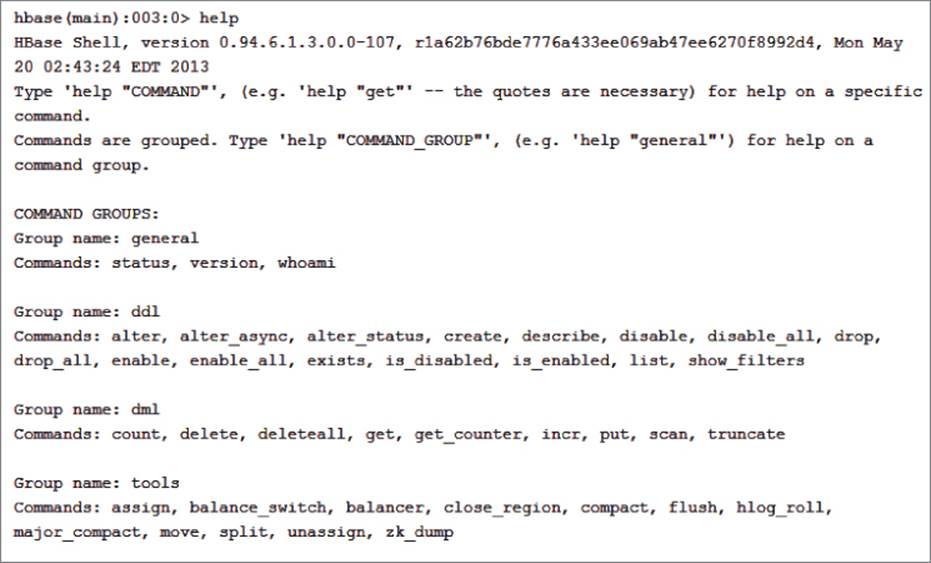
Figure 7.1 Listing the various command groups in the HBase shell.

There are command groups for data definition statements (DDL), data manipulation statements (DML), replication, tools, and security. To list help for a command group, issue the help command followed by the group name in quotation marks. For example, Figure 7.2 shows the help for the DDL command group (only the Alter command is showing).

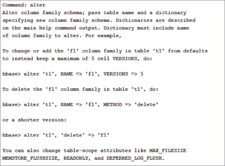
Figure 7.2 Listing help for the DDL command group.

To create a basic table named Stocks with a column family named Price and one named Trade, enter the following code at the command prompt:

create 'Stocks', 'Price','Trade'

To verify that the table has been created, you can use the describe command:

describe 'Stocks'

Figure 7.3 shows the output describing the table attributes.

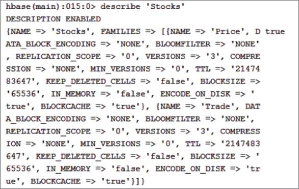
Figure 7.3 Describing the table attributes.

Notice the two column family groups. You can also set attributes for the table/column groups (for example, the number of versions to keep and whether to keep deleted cells).

Now that you've created your table, you're ready to load data into it.

Loading Data into an HBase Table

You can load data into the table in two ways. To load a single value, you use the put command, supplying the table, column, and value. The column is prefixed by the column family. The following code loads a row of stock data into the Stocks table:

put 'Stocks', 'ABXA_12092009','Price:Open','2.55'

put 'Stocks', 'ABXA_12092009','Price:High','2.77'

put 'Stocks', 'ABXA_12092009','Price:Low','2.5'

put 'Stocks', 'ABXA_12092009','Price:Close','2.67'

put 'Stocks', 'ABXA_12092009','Trade:Volume','158500'

To verify that the values have been loaded in the table, you can use the scan command:

scan 'Stocks'

You should see the key/values listed as shown in Figure 7.4. Notice a timestamp has been automatically loaded as part of the key to keep track of versioning.

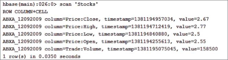
Figure 7.4 Listing key/values.

If the key is already in the table, HBase updates the value and creates a new timestamp for the cell. The old record is still maintained in the table.

Using the HBase shell and the put command illustrates the process of adding a row to the table, but it is not practical in a production setting. You can load data into an HBase table in several other ways. You can use the HBase tools ImportTsv and CompleteBulkLoad. You can also write a MapReduce job or write a custom application using the HBase API. Another option is to use Hive or Pig to load the data. For example, the following code loads data into an HBase table from a CSV file:

StockData = LOAD '/user/hue/StocksTest2.csv' USING PigStorage(',') as

(RowKey:chararray,stock_price_open:long);

STORE StockData INTO 'hbase://StocksTest'

USING org.apache.pig.backend.hadoop.hbase.HBaseStorage('Price:Open');

Now that you know how to load the data into the table, it is now time to see how you read the data from the table.

Performing a Fast Lookup

One of HBase's strengths is its ability to perform fast lookups. HBase supports two data-retrieval operations: get and scan. The get operation returns the cells for a specified row. For example, the following get command is used to retrieve the cell values for a row in the Stocks table. Figure 7.5 shows the resulting output:

get 'Stocks', 'ABXA_12092009'

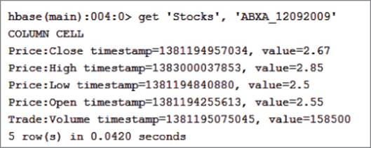
Figure 7.5 Getting the row cell values.

You can also use the get command to retrieve the previous versions of a cell value. The following get command gets the last three versions of the high column. Figure 7.6 shows the output:

get 'Stocks', 'ABXA_12092009', {COLUMN => 'Price:High', VERSIONS => 3}

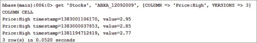
Figure 7.6 Retrieving previous versions of a cell.

You can query the values in the HBase table using the scan command. The following command returns all columns in the Stocks table:

scan 'Stocks'

You can limit the output by passing filters with the scan command. For example, to retrieve just the high price column, you can use the following command:

scan 'Stocks', {COLUMNS => ['Price:High']}

You can also use value-based filters, prefix filters, and timestamp filters. For example, this filter scans for values greater than 2.8:

scan 'Stocks', {FILTER => "ValueFilter(>, 'binary:2.8')"}

HBase provides for fast scanning and lets you create some complex querying through the use of filters. Unfortunately, it is based on the JRuby language and can be quite complex to master. You may want to investigate a tool such as HBase Manager (http://sourceforge.net/projects/hbasemanagergui/), which provides a simple graphical user interface (GUI) to the HBase database.

Loading and Querying HBase

To complete the exercise in this section, you need to download and install the Hortonworks Data Platform (HDP) for Windows from Hortonworks. (Note: At the time of this writing the HBase shell is not yet exposed in HDP for Windows or HDInsight. It is anticipated it will be available in early 2014.) You can set up HDP for Windows on a development server to provide a local test environment that supports a single-node deployment. (For a detailed discussion of installing the Hadoop development environment on Windows, see http://hortonworks.com/products/hdp-windows/.)

In this exercise, you load stock data into an HBase table and query the data using scan filters. The file containing the data is a tab-separated value file named StocksTest.tsv that you can download from http://www.wiley.com/go/microsoftbigdatasolutions.com. The first step is to load the file into the Hadoop file system. Open the Hadoop command-line interface and issue the following command to copy the file (although your paths may differ):

hadoop fs -copyFromLocal

C:\SampleData\StocksTest.tsv /user/test/StockTest.tsv

You can verify the file was loaded by issuing a list command for the directory you placed it in:

hadoop fs -ls /user/test/

The next step is to create the table structure in HBase. Open the HBase shell and enter the following command to create a table named stock_test with three column families (info, price, and trade):

create 'stock_test', 'info','price','trade'

You can use Pig Latin to load the data into the HBase table. Open the Pig command shell and load the TSV file using the PigStorage function. Replace the path below with the path where you loaded StockTest.tsv into HDFS:

StockData = LOAD '/user/test/StockTest.tsv' USING PigStorage() as

(RowKey:chararray,stock_symbol:chararray,date:chararray,

stock_price_open:double,stock_price_close:double,

stock_volume:long);

Now you can load the HBase stock_test table using the HBaseStorage function. This function expects the row key for the table to be pasted first, and then the rest of the fields are passed to the columns designated in the input string:

STORE StockData INTO 'hbase://stock_test'

USING org.apache.pig.backend.hadoop.hbase.HBaseStorage

('info:symbol info:date price:open price:close trade:volume');

To test the load, you can run some scans with various filters passed in. The following scan filters on the symbol to look for the stock symbol ADCT:

SingleColumnValueFilter filter = new SingleColumnValueFilter(

info,

symbol,

CompareOp.EQUAL,

Bytes.toBytes("ADCT")

);

scan.setFilter(filter);

Managing Data with HCatalog

HCatalog creates a table abstraction layer over data stored on an HDFS cluster. This table abstraction layer presents the data in a familiar relational format and makes it easier to read and write data using familiar query language concepts. Originally used in conjunction with Hive and the Hive Query Language (HQL), it has expanded to support other toolsets such as Pig and MapReduce programs. There are also plans to increase the HCatalog support for HBase.

Working with HCatalog and Hive

HCatalog was developed to be used in combination with Hive. HCatalog data structures are defined using Hive's data definition language (DDL) and the Hive metastore stores the HCatalog data structures. Using the command-line interface (CLI), users can create, alter, and drop tables. Tables are organized into databases or are placed in the default database if none are defined for the table. Once tables are created, you can explore the metadata of the tables using commands such as Show Table and Describe Table. HCatalog commands are the same as Hive's DDL commands except that HCatalog cannot issue statements that would trigger a MapReduce job such as Create Table or Select or Export Table.

To invoke the HCatalog CLI, launch the Hadoop CLI and navigate to the bin directory of the HCatalog directory. Enter the command hcat.py, which should result in the output shown in Figure 7.7.To execute a query from the command line, use the -e switch. For example, the following code lists the databases in the metastore:

hcat.py -e "Show Databases"

At this point, the only database listed is the default database.

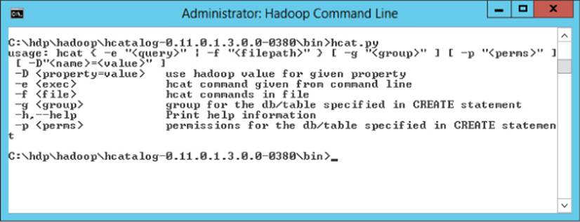
Figure 7.7 Invoking the HCatalog CLI.

Defining Data Structures

You can create databases in HCatalog by issuing a Create Database statement. The following code creates a database named flight to hold airline flight statistics tables:

hcat.py -e "Create Database flight"

To create tables using HCatalog, you use the Create Table command. When creating the table you need to define the column names and data types. HCatalog supports the same data types and is similar to those supported by most database systems such as integer, boolean, float, double, string, binary, and timestamp. Complex types such as the array, map, and struct are also supported. The following code creates an airport table in the flight database to hold airport locations:

Create Table flight.airport

(code STRING, name STRING, country STRING,

latitude double, longitude double)

Once a table is created, you can use the Describe command to see a list of the columns and data types. If you want to see a complete listing of the table metadata, include the Extended keyword, as follows:

Describe Extended flight.airport;

Figure 7.8 shows this command output.

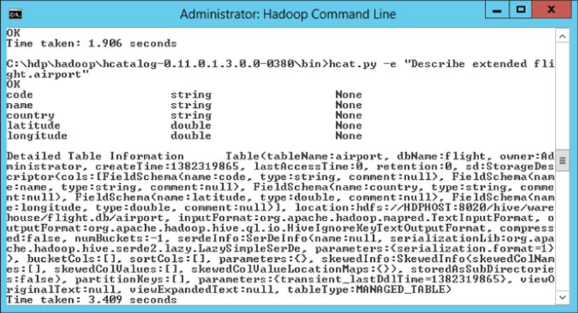
Figure 7.8 Extended description of the airport table.

Once a table is created, you can issue ALTER TABLE statements to do things like changing the table name, alter table properties, change column names, and change column data types. For example, the following command changes the table name:

ALTER TABLE airport RENAME TO us_airports

To add a new column to the table, you use the following code:

ALTER TABLE us_Airports ADD COLUMNS (city String)

You can also drop and truncate a table.

HCatalog supports the creation of views to filter a table. For example, you can create a Canadian airport view using the following command:

Create View canadian_airports as Select * from airport

where country = 'Canada'

Views are not materialized and are only logical structures (although there are plans to eventually support materialized views). When the view is referenced in a query, the view's definition is used to generate the rows. Just as with tables, you can alter views and drop views.

Creating Indexes

When joining tables or performing lookups, it is a good idea for performance to create indexes on the keys used. HCatalog supports the creation of indexes on tables using the CREATE INDEX statement. The following code creates an index on the code column in the us_airports table. Notice that it is passing in a reference to the index handler. Index handlers are pluggable interfaces, so you can create your own indexing technique depending on the requirements:

CREATE INDEX Airport_IDX_1 ON TABLE us_airports (code) AS

'org.apache.hadoop.hive.ql.index.compact.CompactIndexHandler'

with deferred rebuild

The deferred rebuild command is used to defer rebuilding the index until the table is loaded. After the load, you need to issue an ALTER statement to rebuild the index to reflect the changes in the data:

ALTER INDEX Airport_IDX_1 ON us_airports REBUILD

As with most data structures, you can delete an index by issuing the DROP command. The CompactIndexHandler creates an index table in the database to hold the index values. When the index is dropped, the underlying index table is also dropped:

DROP INDEX Airport_IDX_1 ON us_airports

Along with indexing, another way to improve query performance is through partitioning. In the next section, you will see how you can partition tables in HCatalog.

Creating Partitions

When working with large data stores, you can often improve queries by partitioning the data. For example, if queries are retrieved using a date value to restrict the results, a partition on dates will improve performance.

To create a partition on a table, you use the partitioned-by command as part of the Create Table statement. The following statement creates a table partitioned by the date column:

Create Table flightData_Partitioned (airline_cd int,airport_cd string,

delay int,dep_time int) Partitioned By(flight_date string);

Using the describe command, you can view partition information for the table, as shown in Figure 7.9.

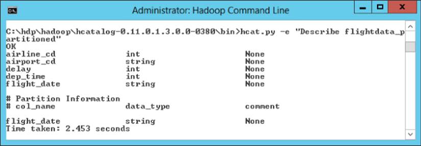
Figure 7.9 Viewing partition information.

You can create partitions on multiple columns, which results in a separate data directory for each distinct combination of values from the partition columns. For example, it may be beneficial to partition the flight data table by both the flight date and airport code depending on the amount of data and the types of queries. Another option is to further bucket the partitions using Clustered By and order the data in the buckets with a Sorted By command. The following statement creates a flight data table partitioned by flight date, bucketed by airport code, and sorted by departure time:

Create Table flightData_Bucketed (airline_cd int,airport_cd string,

delay int,dep_time int) Partitioned By(flight_date string)

Clustered By(airport_cd) Sorted By(dep_time) into 25 buckets;

When loading data into a partitioned table, it is up to you to ensure that the data is loaded into the right partition. You can use Hive to load the tables directly from a file. For example, the following statement is used to load a file containing daily flight data into a table partitioned by date:

LOAD DATA INPATH '/flight/data/flightdata_2013-01-01.txt'

INTO TABLE flightdata PARTITION(date='2013-01-01')

You can also use Hive to load data from one table into another table. For example, you may want to load data from a staging table into the partitioned tables, as illustrated by the following statement:

FROM flightdata_stg fds

INSERT OVERWRITE TABLE flightdata PARTITION(flight_date='2013-01-01')

SELECT fds.airline_cd, fds.airport_cd, fds.delay, fds.dep_time

WHERE fds.flight_date = '2013-01-01'

To load into multiple partitions, you can create a multi-insert statement as follows:

FROM flightdata_stg fds

INSERT OVERWRITE TABLE flightdata PARTITION(flight_date='2013-01-01')

SELECT fds.airline_cd, fds.airport_cd, fds.delay, fds.dep_time

WHERE fds.flight_date = '2013-01-01'

INSERT OVERWRITE TABLE flightdata PARTITION(flight_date='2013-01-02')

SELECT fds.airline_cd, fds.airport_cd, fds.delay, fds.dep_time

WHERE fds.flight_date = '2013-01-02'

If you have a table partitioned on more than one column, HCatalog supports dynamic partitioning. This allows you to load more efficiently without the need to know all the partition values ahead of time. To use dynamic partitioning, you need the top-level partition to be static, and the rest can be dynamic. For example, you could create a static partition on month and a dynamic partition on date. Then you could load the dates for the month in one statement. The following statement dynamically creates and inserts data into a date partition for a month's worth of data:

FROM flightdata_stg fds INSERT OVERWRITE TABLE flightdata

PARTITION(flight_month='01',flight_date)

SELECT fds.airline_cd, fds.airport_cd, fds.delay, fds.dep_time,

fds.flight_date WHERE fds.flight_month = '01'

One caveat to note is that the dynamic partition columns are selected by order and are the last columns in the select clause.

Integrating HCatalog with Pig and Hive

Although originally designed to provide the metadata store for Hive, HCatalog's role has greatly expanded in the Hadoop ecosystem. It integrates with other tools and supplies read and write interfaces for Pig and MapReduce. It also integrates with Sqoop, which is a tool designed to transfer data back and forth between Hadoop and relational databases such as SQL Server and Oracle. HCatalog also exposes a REST interface so that you can create custom tools and applications to interact with Hadoop data structures. In addition, HCatalog contains a notification service so that it can notify workflow tools such as Oozie when data has been loaded or updated.

Another key feature of HCatalog is that it allows developers to share data and structures across internal toolsets like Pig and Hive. You do not have to explicitly type the data structures in each program. This allows us to use the right tool for the right job. For example, we can load data into Hadoop using HCatalog, perform some ETL on the data using Pig, and then aggregate the data using Hive. After the processing, you could then send the data to your data warehouse housed in SQL Server using Sqoop. You can even automate the process using Oozie.

To complete the following exercise, you need to download and install the HDP for Windows from Hortonworks. You can set up HDP for Windows on a development server to provide a local test environment that supports a single-node deployment. (For a detailed discussion of installing the Hadoop development environment on Windows, see http://hortonworks.com/products/hdp-windows/.)

In this exercise, we analyze sensor data collected from HVAC systems monitoring the temperatures of buildings. You can download the sensor data from http://www.wiley.com/go/microsoftbigdatasolutions. There should be two files, one with sensor data (HVAC.csv) and a file containing building information (building.csv). After extracting the files, load the data into a staging table using HCatalog and Hive:

1. Open the Hive CLI. Because Hive and HCatalog are so tightly coupled, you can write HCatalog commands directly in the Hive CLI. As a matter of fact, you may recall that HCatalog actually uses a subset of Hive DDL statements. Create the sensor staging table with the following code:

2. CREATE TABLE sensor_stg(dt String, time String, target_tmp Int,

3. actual_tmp Int, system Int, system_age Int,building_id Int)

ROW FORMAT DELIMITED FIELDS TERMINATED BY ',';

4. Load the data into the staging table:

5. LOAD DATA Local INPATH 'C:\SampleData\HVAC.csv'

INTO TABLE sensor_stg;

6. Use the following statement to view the data to verify that it loaded. Your data should look similar to Figure 7.10:

Select * from sensor_stg Limit 10;

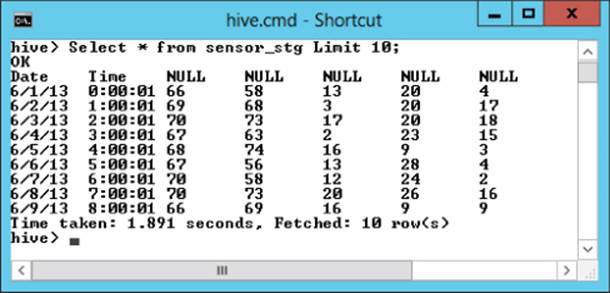
Figure 7.10 Sample sensor data.

7. Using the same process, load the building data into a staging table:

8. CREATE TABLE building_stg(building_id Int, mgr String,

9. building_age Int,

10. hvac_type String, country String)

11. ROW FORMAT DELIMITED FIELDS TERMINATED BY ',';

12. LOAD DATA Local INPATH 'C:\SampleData\building.csv'

13. INTO TABLE building_stg;

Select * from building_stg Limit 10;

14.Create tables to hold the processed data. The sensor table is partitioned by the date:

15. CREATE TABLE sensor(time String, target_tmp Int,

16. actual_tmp Int,delta_tmp Int, building_id Int)

17. PARTITIONED BY (dt String);

18. CREATE TABLE building(building_id Int,

building_age Int, hvac_type String);

19.Because you are going to join the tables using the building ID, you are going to create indexes for the tables using this column:

20. CREATE INDEX Building_IDX_1 ON TABLE sensor (building_id)

21. AS 'org.apache.hadoop.hive.ql.index.compact.CompactIndexHandler'

22. with deferred rebuild;

23. CREATE INDEX Building_IDX_2 ON TABLE building (building_id)

24. AS 'org.apache.hadoop.hive.ql.index.compact.CompactIndexHandler'

with deferred rebuild;

Now you can use Pig to extract, transform, and load the data from staging tables into the analysis tables.

25.Open the Hadoop CLI and browse to the bin directory of the Pig installation folder. Issue the following command to launch the Pig CLI, passing in the switch to use HCatalog:

pig.cmd -useHCatalog;

This will launch the Grunt, the Pig CLI.

26.Issue the following Pig Latin script to load the data from the staging table:

27. SensorData = load 'sensor_stg'

using org.apache.hcatalog.pig.HCatLoader();

You should see an output message indicating that a connection to the metastore is established.

28.To ensure that the data is loaded, you can issue a Dump command to output the data to the screen (which will take a few minutes):

Dump SensorData;

29.Use the following code to filter out nulls and calculate the temperature deltas:

30. FilteredData = Filter SensorData By building_id is not null;

31. ProcessedData = Foreach FilteredData Generate dt, time, target_tmp,

actual_tmp,target_tmp - actual_tmp as delta_tmp,building_id;

32.The final step is to load the processed data into the sensor table:

33. STORE ProcessedData INTO 'sensor' USING

org.apache.hcatalog.pig.HCatStorer();

Once the table loads, you can close the CLI.

34.Open the Hive CLI and issue the following query to verify that the sensor table has been loaded. Your output should look similar to Figure 7.11. Notice that the data is all coming from the same partition (date):

Select * from sensor Limit 10;

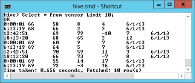
Figure 7.11 Selecting sensor data.

35.Load the building table with the following query:

36. From building_stg bs

37. Insert Overwrite Table building

select bs.building_id, bs.building_age, bs.hvac_type;

38.Now that the tables are loaded, you need to build the indexes:

39. ALTER INDEX Building_IDX_1 ON sensor REBUILD;

ALTER INDEX Building_IDX_2 ON building REBUILD;

After the index has been built, the data is now ready to analyze.

You can use Hive to query and aggregate the data. The following query determines the maximum temperature difference between target and actual temperatures for each day and HVAC type:

select max(s.delta_tmp), s.dt, b.hvac_type

from sensor s join building b on (s.building_id = b.building_id)

Group By s.dt, b.hvac_type;

In Chapter 11, “Visualizing Big Data with Microsoft BI,” you will see how you can use the Hive ODBC connector to load and analyze the data in Microsoft's BI toolset.

Using HBase or Hive as a Data Warehouse

Although both HBase and Hive are both considered data warehouse structures, they differ significantly as to how they store and query data. Hive is more like a traditional data warehouse reporting system. It structures the data in a set of tables that you can join, aggregate, and query on using a query language (Hive Query Language [HQL]) that is very similar to the SQL, which most database developers are already used to working with. This relieves you from having to write MapReduce code. The downside to Hive is it can take a long time to process through the data and is not intended to give clients instant results.

Hive is usually used to run processing through scheduled jobs and then load the results into a summary type table that can be queried on by client applications. One of the strengths of Hive and HCatalog is the ability to pass data between traditional relational databases such as SQL Server. A good use case for Hive and HCatalog is to load large amounts of unstructured data, aggregate the data, and push the results back to SQL Server where analysts can use the Microsoft BI toolset to explore the results. Another point to consider is that Hive and HCatalog do not allow data updates. When you load the data, you can either replace or append. This makes loading large amounts of data extremely fast, but limits your ability to track changes.

HBase, however, is a key/value data store that allows you to read, write, and update data. It is designed to allow quick reads of random access data from large amounts of data based on the key values. It is not designed to provide fast loading of large data sets, but rather quick updates and inserts of single sets of data that may be streaming in from a source. It also is not designed to perform aggregations of the data. It has a query language based on JRuby that is very unfamiliar to most SQL developers. Having said that, HBase will be your tool of choice under some circumstances. Suppose, for example, that you have a huge store of e-mail messages and you need to occasionally pull one for auditing. You may also tag the e-mails with identifying fields that may occasionally need updating. This is an excellent use case for HBase.

If you do need to aggregate and process the data before placing it into a summary table that needs to be updated, you can always use HBase and Hive together. You can load and aggregate the data with Hive and push the results to a table in HBase, where the data summary statistics can be updated.

Summary

This chapter examined two tools that you can use to create structure on top of your big data stored in HDFS. HBase is a tool that creates key/value tuples on top of the data and stores the key values in a columnar storage structure. Its strength is that it enables fast lookups and supports consistency when updating the data. The other tool, HCatalog, offers a relational table abstraction layer over HDFS. Using the HCatalog abstraction layer allows query tools such as Pig and Hive to treat the data in a familiar relational architecture. It also permits easier exchange of data between the HDFS storage and relational databases such as SQL Server and Oracle.