Excel® 2016 Formulas and Functions (2016)
Part I: Mastering Excel Ranges and Formulas
1. Getting the Most Out of Ranges
In This Chapter
Advanced Range-Selection Techniques
Data Entry in a Range
Filling a Range
Creating a Series
Advanced Range Copying and Pasting
Clearing a Range
Applying Conditional Formatting to a Range
Other than performing data-entry chores, you probably spend most of your Excel life working with ranges in some way. Whether you’re copying, moving, formatting, naming, or filling them, ranges are a big part of Excel’s day-to-day operations. And why not? After all, working with a range of cells is a lot easier than working with each cell individually. For example, suppose that you want to know the average of a column of numbers running from B1 to B30. You could enter all 30 cells as arguments in the AVERAGE function, but I’m assuming that you have a life to lead away from your computer screen. Typing =AVERAGE(B1:B30) is decidedly quicker (and probably more accurate).
In other words, ranges save time, and they save wear and tear on your typing fingers. But there’s more to ranges than that. Ranges are powerful tools that can unlock the hidden depths of Excel. So, the more you know about ranges, the more you’ll get out of your Excel investment, particularly when it comes to building formulas. This chapter takes you beyond the range routine and shows you some techniques for taking full advantage of Excel’s range capabilities.
Advanced Range-Selection Techniques
As you work with Excel, you’ll come across three situations when you’ll need to select a cell range:
![]() When a dialog box field requires a range input
When a dialog box field requires a range input
![]() While entering a function argument
While entering a function argument
![]() Before selecting a command that uses a range input
Before selecting a command that uses a range input
In a dialog box field or function argument, the most straightforward way to select a range is to enter the range coordinates by hand. You do this by typing the address of the upper-left cell (called the anchor cell), followed by a colon and then the address of the lower-right cell. To use this method, either you must be able to see the range you want to select or you must know in advance the range coordinates you want. Because this is often not the case, most people don’t type the range coordinates directly; instead, they select ranges using either the mouse or the keyboard.
This chapter assumes that you know the basic, garden-variety range-selection techniques. Therefore, the next few sections show you a few advanced techniques that can make your selection chores faster and easier.
Mouse Range-Selection Tricks
Keep these handy techniques in mind when using a mouse to select a range:
![]() When selecting a rectangular, contiguous range, if you select the wrong lower-right corner, your range will be either too big or too small. To fix it, hold down the Shift key and click the correct lower-right cell. The range adjusts automatically.
When selecting a rectangular, contiguous range, if you select the wrong lower-right corner, your range will be either too big or too small. To fix it, hold down the Shift key and click the correct lower-right cell. The range adjusts automatically.
![]() After selecting a large range, you’ll often no longer see the active cell because you may have scrolled it off the screen. If you need to see the active cell before continuing, you can either use the scroll bars to bring it into view or press Ctrl+Backspace.
After selecting a large range, you’ll often no longer see the active cell because you may have scrolled it off the screen. If you need to see the active cell before continuing, you can either use the scroll bars to bring it into view or press Ctrl+Backspace.
![]() You can use Excel’s Extend mode as an alternative method for using the mouse to select a rectangular, contiguous range. Click the upper-left cell of the range you want to select, press F8 to enter Extend mode (you see “Extend Selection” in the status bar), and then click the lower-right cell of the range. Excel selects the entire range. Press F8 again to turn off Extend mode.
You can use Excel’s Extend mode as an alternative method for using the mouse to select a rectangular, contiguous range. Click the upper-left cell of the range you want to select, press F8 to enter Extend mode (you see “Extend Selection” in the status bar), and then click the lower-right cell of the range. Excel selects the entire range. Press F8 again to turn off Extend mode.
![]() If the cells you want to work with are scattered willy-nilly throughout the sheet, you need to combine them into a noncontiguous range. The secret to defining a noncontiguous range is to hold down the Ctrl key while selecting the cells. That is, you first select a cell or range you want to include in the noncontiguous range, press and hold down the Ctrl key, and then select the other cells or rectangular ranges you want to include in the noncontiguous range.
If the cells you want to work with are scattered willy-nilly throughout the sheet, you need to combine them into a noncontiguous range. The secret to defining a noncontiguous range is to hold down the Ctrl key while selecting the cells. That is, you first select a cell or range you want to include in the noncontiguous range, press and hold down the Ctrl key, and then select the other cells or rectangular ranges you want to include in the noncontiguous range.
Caution
When you’re selecting a noncontiguous range, always press and hold down the Ctrl key after you’ve selected your first cell or range. Otherwise, Excel includes the currently selected cell or range as part of the noncontiguous range. This action could create a circular reference in a function if you are defining the range as one of the function’s arguments.
![]() If you’re not sure what a “circular reference” is, see “Fixing Circular References,” p. 118.
If you’re not sure what a “circular reference” is, see “Fixing Circular References,” p. 118.
Keyboard Range-Selection Tricks
Excel comes with a couple of tricks to make selecting a range via the keyboard easier or more efficient:
![]() If you want to select a contiguous range that contains data, there’s an easy way to select the entire range: Select any cell within the range and then press Ctrl+* or Ctrl+A. (For the latter, if you then press Ctrl+A a second time, Excel selects the entire sheet.)
If you want to select a contiguous range that contains data, there’s an easy way to select the entire range: Select any cell within the range and then press Ctrl+* or Ctrl+A. (For the latter, if you then press Ctrl+A a second time, Excel selects the entire sheet.)
Caution
The Ctrl+A behavior in Excel 2013 and later is actually more bizarre than I’ve let on so far. Pressing Ctrl+A twice to select the entire sheet works only if the current cell is within a range that contains data or if the current cell is between two ranges that have only a single column or row between them. If the current cell is one row above or one column to the left of a range with data, pressing Ctrl+A selects the empty row or column and the range but pressing Ctrl+A again does nothing. If the current cell is not adjacent to a range or has no data to the right or below, then pressing Ctrl+A selects the entire sheet.
![]() To select a contiguous range where the current cell becomes the upper-left corner of the selection, press Ctrl+Shift+End.
To select a contiguous range where the current cell becomes the upper-left corner of the selection, press Ctrl+Shift+End.
![]() If the range you select is so large that all the cells don’t fit on the screen, you can scroll through the selected cells by activating the Scroll Lock key, if your keyboard has one. (“Scroll Lock” appears in the status bar.) When Scroll Lock is on, pressing the arrow keys (or Page Up and Page Down) scrolls you through the cells while keeping the selection intact.
If the range you select is so large that all the cells don’t fit on the screen, you can scroll through the selected cells by activating the Scroll Lock key, if your keyboard has one. (“Scroll Lock” appears in the status bar.) When Scroll Lock is on, pressing the arrow keys (or Page Up and Page Down) scrolls you through the cells while keeping the selection intact.
Working with 3D Ranges
A 3D range is a range selected on multiple worksheets. This is a powerful concept because it means that you can select a range on two or more sheets and then enter data, apply formatting, or give a command, and the operation will affect all the ranges simultaneously. This is useful when you’re working with a multisheet model where some or all the labels are the same on each sheet. For example, in a workbook of expense calculations where each sheet details the expenses from a different division or department, you might want the label “Expenses” to appear in cell A1 on each sheet.
To create a 3D range, first you need to group the worksheets you want to work with. To select multiple sheets, use any of the following techniques:
![]() To select adjacent sheets, click the tab of the first sheet, hold down the Shift key, and click the tab of the last sheet.
To select adjacent sheets, click the tab of the first sheet, hold down the Shift key, and click the tab of the last sheet.
![]() To select nonadjacent sheets, click the tab of a sheet you want to include in the group, hold down the Ctrl key, and click the tab of each additional sheet you want to include in the group.
To select nonadjacent sheets, click the tab of a sheet you want to include in the group, hold down the Ctrl key, and click the tab of each additional sheet you want to include in the group.
![]() To select all the sheets in a workbook, right-click any sheet tab and click the Select All Sheets command.
To select all the sheets in a workbook, right-click any sheet tab and click the Select All Sheets command.
When you’ve selected your sheets, each tab is highlighted, and “[Group]” appears in the workbook title bar. To ungroup the sheets, click a tab that isn’t in the group. Alternatively, you can right-click one of the group’s tabs and select the Ungroup Sheets command from the shortcut menu.
With the sheets now grouped, you create your 3D range by switching to any of the grouped sheets and then selecting a range. Excel selects the same cells in all the other sheets in the group.
You can also type in a 3D range by hand when, say, entering a formula. Here’s the general format for a 3D reference:
FirstSheet:LastSheet!ULCorner:LRCorner
Here, FirstSheet is the name of the first sheet in the 3D range, LastSheet is the name of the last sheet, and ULCorner and LRCorner define the cell range you want to work with on each sheet. (Note that UL refers to Upper Left and LR refers to Lower Right.) For example, to specify the range A1:E10 on worksheets Sheet1, Sheet2, and Sheet3, use the following reference:
Sheet1:Sheet3!A1:E10
Caution
If one or both of the sheet names used in the 3D reference contain a space, be sure to enclose the sheet names in single quotation marks, as in this example:
'First Quarter:Fourth Quarter'!A1:F16
Caution
After you’re finished with the 3D range, be sure to ungroup the worksheets so that you don’t accidentally overwrite data or make other inadvertent changes in the grouped sheets.
You normally use 3D references in worksheet functions that accept them. These functions include AVERAGE(), COUNT(), COUNTA(), MAX(), MIN(), PRODUCT(), STDEV(), STDEVP(), SUM(), VAR(), and VARP(). (You’ll learn about these and other functions in Part II, “Harnessing the Power of Functions.”)
Selecting a Range Using Go To
For very large ranges, Excel’s Go To command comes in handy. You normally use the Go To command to jump quickly to a specific cell address or range name. The following steps show you how to exploit this power to select a range:
1. Select the upper-left cell of the range.
2. Select Home, Find & Select, Go To (or press F5 or Ctrl+G). The Go To dialog box appears, as shown in Figure 1.1.
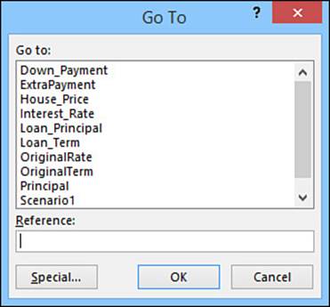
Figure 1.1 You can use the Go To dialog box to easily select a large range.
3. Use the Reference text box to enter the cell address of the lower-right corner of the range.
Tip
You also can select a range using Go To by entering the range coordinates in the Reference text box.
4. Hold down the Shift key and click OK. Excel selects the range.
Tip
Another way to select very large ranges is to select View, Zoom and click a reduced magnification in the Zoom dialog box (say, 50% or 25%; you can also click and drag the Zoom slider in the status bar or hold down Ctrl and scroll the mouse wheel). You can then use this “big picture” view to select your range.
Using the Go To Special Dialog Box
You normally select cells according to their position within a worksheet. However, Excel includes a powerful feature that enables you to select cells according to their contents or other special properties. If you select Home, Find & Select, Go To Special (or click the Special button in the Go To dialog box), the Go To Special dialog box appears, as shown in Figure 1.2.
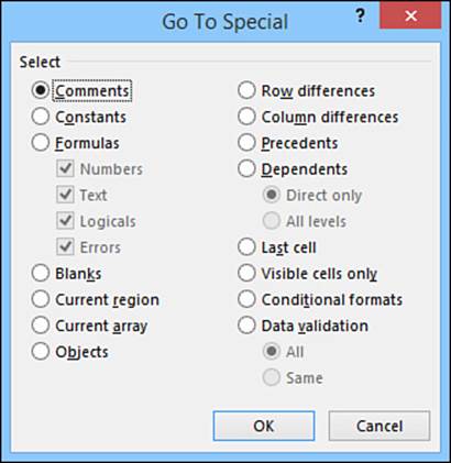
Figure 1.2 Use the Go To Special dialog box to select cells according to their contents, formula relationships, and more.
Selecting Cells by Type
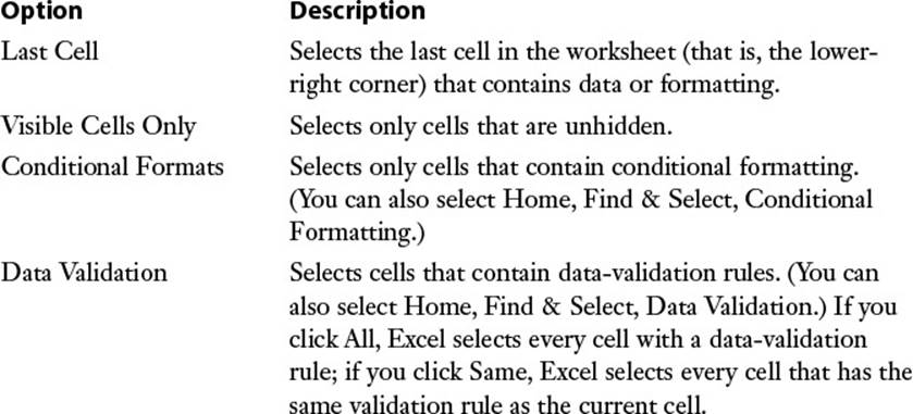
The Go To Special dialog box contains many options, but only four of them enable you to select cells according to the type of contents they contain. Table 1.1 summarizes these four options. (The next few sections discuss the other Go To Special options.)
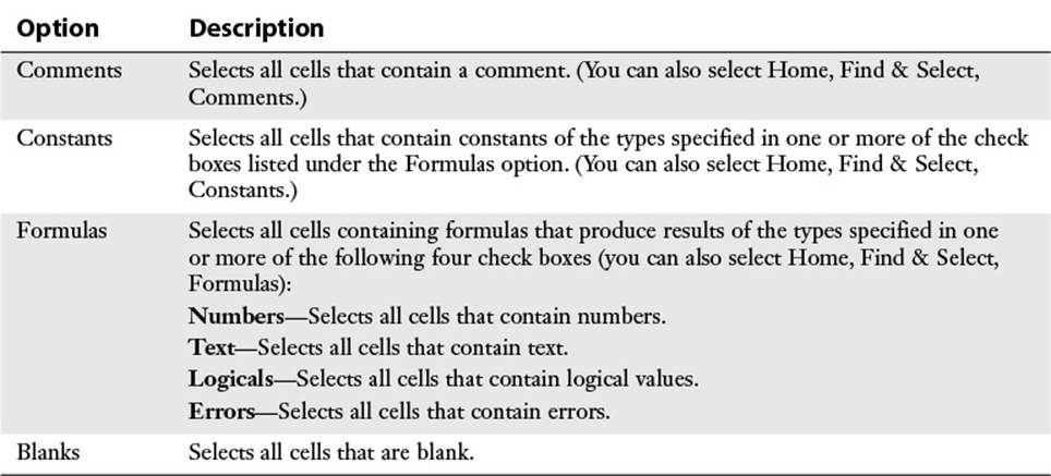
Table 1.1 Options for Selecting a Cell by Type
Selecting Adjacent Cells
The Go To Special dialog box gives you two options for selecting cells adjacent to the active cell. Click the Current Region option to select a rectangular range that extends to the right from the active cell to (but not including) the next empty column and down from the active cell to (but not including) the next empty row.
If the active cell is part of an array, click the Current Array option to select all the cells in the array.
![]() For an in-depth discussion of Excel arrays, see “Working with Arrays,” p. 87.
For an in-depth discussion of Excel arrays, see “Working with Arrays,” p. 87.
Selecting Cells by Differences
Excel also enables you to select cells by comparing rows or columns of data and selecting only those cells that are different. The following steps show you how it’s done:
1. Select the rows or columns you want to compare. (Make sure that the active cell is in the row or column with the comparison values you want to use.)
2. Display the Go To Special dialog box and click one of the following options:
• Row Differences—This option uses the data in the active cell’s column as the comparison values. Excel selects the cells in the corresponding rows that are different.
• Column Differences—This option uses the data in the active cell’s row as the comparison values. Excel selects the cells in the corresponding columns that are different.
3. Click OK.
For example, Figure 1.3 shows a selected range of numbers. The values in column B are the budget numbers assigned to all the company’s divisions; the values in columns C and D are the actual numbers achieved by the East Division and the West Division, respectively. Suppose you want to know the items for which a division ended up either under or over the budget. In other words, you want to compare the numbers in columns C and D with those in column B, and then you want to select the ones in C and D that are different. Because you’re comparing rows of data, you’d select the Row Differences option from the Go To Special dialog box. Figure 1.4 shows the results.
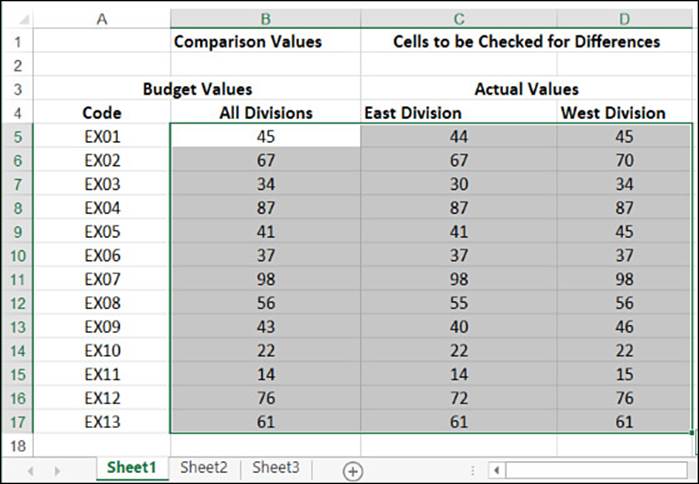
Figure 1.3 Before using the Go To Special feature that compares rows (or columns) of data, select the entire range of cells involved in the comparison.
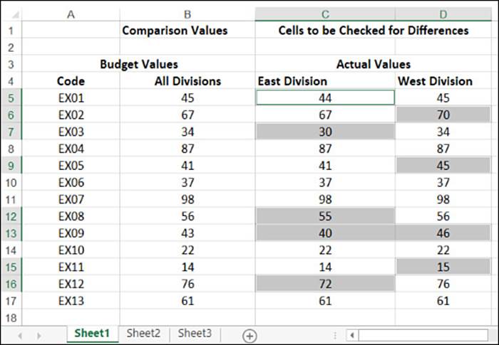
Figure 1.4 After running the Row Differences option, Excel shows those rows in columns C and D that are different from the value in column B.
Note
You can download this chapter’s sample workbooks at www.mcfedries.com/books/book.php?title=excel-2016-formulas-and-functions.
Selecting Cells by Reference
If a cell contains a formula, Excel defines the cell’s precedents as those cells that the formula refers to. For example, if cell A4 contains the formula =SUM(A1:A3), cells A1, A2, and A3 are the precedents of A4. A direct precedent is a cell referred to explicitly in the formula. In the preceding example, A1, A2, and A3 are direct precedents of A4. An indirect precedent is a cell referred to by a precedent. For example, if cell A1 contains the formula =B3*2, cell B3 is an indirect precedent of cell A4.
Excel also defines a cell’s dependents as those cells with a formula that refers to the cell. In the preceding example, cell A4 would be a dependent of cell A1. Like precedents, dependents can be direct or indirect.
Note
Think of dependents this way: The value that appears in cell A4 depends on the value that’s entered in cell A1.
The Go To Special dialog box enables you to select precedents and dependents as described in these steps:
1. Select the range you want to work with.
2. Display the Go To Special dialog box.
3. Click either the Precedents option or the Dependents option.
4. Click the Direct Only option to select only direct precedents or dependents. If you need to select both the direct and the indirect precedents or dependents, click the All Levels option.
5. Click OK.
Other Go To Special Options
The Go To Special dialog box includes a few more options to help you in your range-selection chores:
![]() To learn about conditional formatting, see “Applying Conditional Formatting to a Range,” p. 25.
To learn about conditional formatting, see “Applying Conditional Formatting to a Range,” p. 25.
![]() To learn about data validation, see “Applying Data-Validation Rules to Cells,” p. 100.
To learn about data validation, see “Applying Data-Validation Rules to Cells,” p. 100.
Shortcut Keys for Selecting via Go To
Table 1.2 lists the shortcut keys you can use to run many of the Go To Special operations.
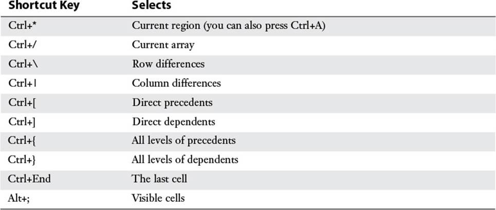
Table 1.2 Shortcut Keys for Selecting Precedents and Dependents
Data Entry in a Range
If you know in advance which range you’ll use for data entry, you can save yourself some time and keystrokes by selecting the range before you begin. As you enter your data in each cell, use the keys listed in Table 1.3 to navigate the range.
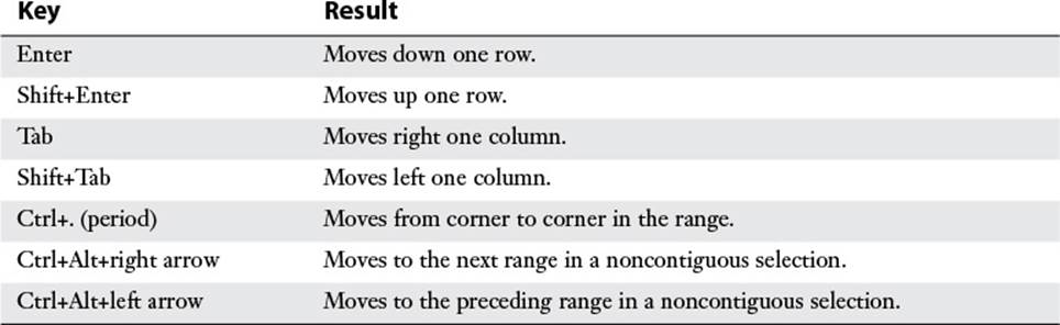
Table 1.3 Navigation Keys for a Selected Range
The advantage of this technique is that the active cell never leaves the range. For example, if you press Enter after adding data to a cell in the last row of the range, the active cell moves back to the top row and over one column.
Filling a Range
If you need to fill a range with a particular value or formula, Excel gives you two methods:
![]() Select the range you want to fill, type the value or formula, and press Ctrl+Enter. Excel fills the entire range with whatever you entered in the formula bar. If you entered a formula with relative cell references, Excel adjusts those references as it fills the range.
Select the range you want to fill, type the value or formula, and press Ctrl+Enter. Excel fills the entire range with whatever you entered in the formula bar. If you entered a formula with relative cell references, Excel adjusts those references as it fills the range.
![]() Enter the initial value or formula, select the range you want to fill (including the initial cell), and select Home, Fill. Then select the appropriate command from the submenu that appears. For example, if you’re filling a range down from the initial cell, select the Down command. If you’ve selected multiple sheets, use Home, Fill, Across Worksheets to fill the range in each worksheet.
Enter the initial value or formula, select the range you want to fill (including the initial cell), and select Home, Fill. Then select the appropriate command from the submenu that appears. For example, if you’re filling a range down from the initial cell, select the Down command. If you’ve selected multiple sheets, use Home, Fill, Across Worksheets to fill the range in each worksheet.
Tip
Press Ctrl+D to select Home, Fill, Down; press Ctrl+R to select Home, Fill, Right.
Using the Fill Handle
The fill handle is the small green square in the lower-right corner of the active cell or range. This versatile little tool can do many useful things, including create a series of text or numeric values and fill, clear, insert, and delete ranges. The next few sections show you how to use the fill handle to perform each of these operations.
Using AutoFill to Create Text and Numeric Series
Worksheets often use text series (such as January, February, March, or Sunday, Monday, Tuesday) and numeric series (such as 1, 3, 5, or 2014, 2015, 2016). Instead of entering these series by hand, you can use the fill handle to create them automatically. This handy feature is called AutoFill, and the following steps show you how it works:
1. For a text series, select the first cell of the range you want to use and enter the initial value. For a numeric series, enter the first two values and then select both cells.
2. Position the mouse pointer over the fill handle. The pointer changes to a plus sign (+).
3. Click and drag the mouse pointer until the gray border encompasses the range you want to fill. If you’re not sure where to stop, keep your eye on the pop-up value that appears near the mouse pointer and shows you the series value of the last selected cell.
4. Release the mouse button. Excel fills in the range with the series.
When you release the mouse button after using AutoFill, Excel not only fills in the series but also displays the Auto Fill Options button. To see the options, move your mouse pointer over the button and then click the downward-pointing arrow to drop down the list. The options you see depend on the type of series you created. (See “Creating a Series,” later in this chapter, for details on some of the options you might see.) However, you’ll usually see at least the following five:
![]() Copy Cells—Choose this option to fill the range by copying the original cell or cells.
Copy Cells—Choose this option to fill the range by copying the original cell or cells.
![]() Fill Series—Choose this option to get the default series fill.
Fill Series—Choose this option to get the default series fill.
![]() Fill Formatting Only—Choose this option to apply only the original cell’s formatting to the selected range.
Fill Formatting Only—Choose this option to apply only the original cell’s formatting to the selected range.
![]() Fill Without Formatting—Choose this option to fill the range with the series data but without the formatting of the original cell.
Fill Without Formatting—Choose this option to fill the range with the series data but without the formatting of the original cell.
![]() Flash Fill—Choose this option to fill the range based on the pattern you specified in the original cell. See “Flash-Filling a Range,” later in this chapter, for the details.
Flash Fill—Choose this option to fill the range based on the pattern you specified in the original cell. See “Flash-Filling a Range,” later in this chapter, for the details.
Figure 1.5 shows several series created with the fill handle. (The shaded cells are the initial fill values.) In particular, notice that Excel increments any text value that includes a numeric component, such as Quarter 1 (see column E) and Customer 1001 (see column F).
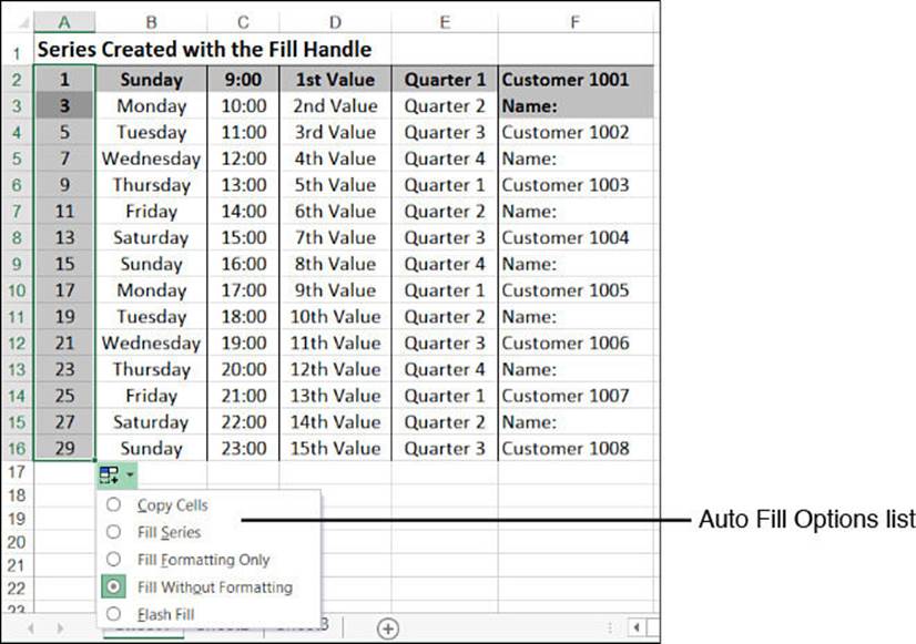
Figure 1.5 Some sample series created with the fill handle. Shaded entries are the initial fill values.
Keep the following guidelines in mind when using the fill handle to create a series:
![]() Clicking and dragging the handle down or to the right increments the values. Clicking and dragging up or to the left decrements the values.
Clicking and dragging the handle down or to the right increments the values. Clicking and dragging up or to the left decrements the values.
![]() The fill handle recognizes standard abbreviations such as Jan (January) and Sun (Sunday).
The fill handle recognizes standard abbreviations such as Jan (January) and Sun (Sunday).
![]() To vary the series interval for a text series, enter the first two values of the series and then select both of them before clicking and dragging. For example, entering 1st and 3rd produces the series 1st, 3rd, 5th, and so on.
To vary the series interval for a text series, enter the first two values of the series and then select both of them before clicking and dragging. For example, entering 1st and 3rd produces the series 1st, 3rd, 5th, and so on.
![]() If you use three or more numbers as the initial values for the fill handle series, Excel creates a “best fit” or “trend” line.
If you use three or more numbers as the initial values for the fill handle series, Excel creates a “best fit” or “trend” line.
![]() To learn more about using Excel for trend analysis, see Chapter 16, “Using Regression to Track Trends and Make Forecasts,” p. 371.
To learn more about using Excel for trend analysis, see Chapter 16, “Using Regression to Track Trends and Make Forecasts,” p. 371.
Creating a Custom AutoFill List
As you saw in the previous section, Excel recognizes certain values, such as January, Sunday, and Quarter 1, as parts of larger lists. When you drag the fill handle from a cell containing one of these values, Excel fills the cells with the appropriate series. However, you’re not stuck with just the few lists that Excel recognized out of the box. Instead, you’re free to define your own AutoFill lists, as described in the following steps:
1. Select File, Options to display the Excel Options dialog box.
2. Click Advanced and then click Edit Custom Lists to open the Custom Lists dialog box.
3. In the Custom Lists box, click New List. An insertion point appears in the List Entries box.
4. Type an item from your list into the List Entries box and press Enter. Repeat this step for each item. (Make sure you add the items in the order in which you want them to appear in the series.) Figure 1.6 shows an example.
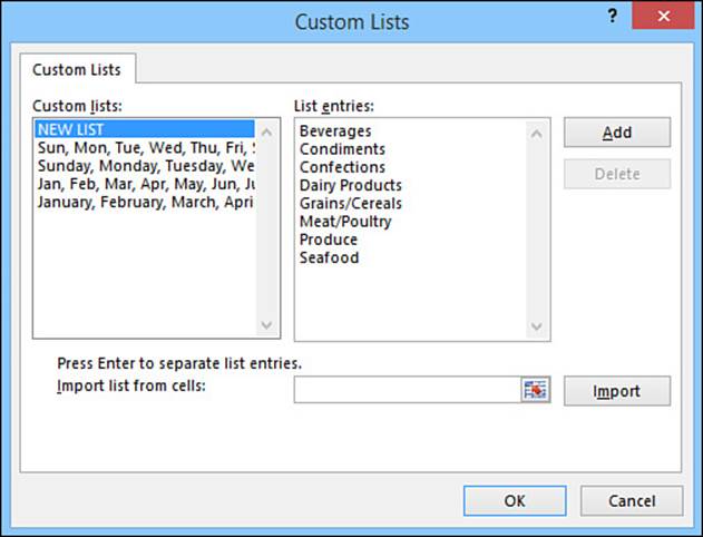
Figure 1.6 Use the Custom Lists tab to create your own lists that Excel can fill in automatically, using the AutoFill feature.
Tip
If you already have the list in a worksheet range, don’t bother entering each item by hand. Instead, activate the Import List from Cells edit box and enter a reference to the range (either by typing the reference or selecting the cells directly on the worksheet). Click the Import button to add the list to the Custom Lists box.
5. Click Add to add the list to the Custom Lists box.
6. Click OK and then click OK again to return to the worksheet.
Note
If you need to delete a custom list, select it in the Custom Lists box and then click Delete.
Using the Fill Handle to Fill a Range
You can use the fill handle to fill a range with a value or formula. To do this, enter your initial value or formula and then click and drag the fill handle over the destination range. When you release the mouse button, Excel fills the range.
Note that if the initial cell contains a formula with relative references, Excel adjusts the references accordingly. For example, suppose the initial cell contains the formula =A1. If you fill down, the next cell will contain the formula =A2, the next will contain =A3, and so on.
![]() For information on relative references, see “Understanding Relative Reference Format,” p. 62.
For information on relative references, see “Understanding Relative Reference Format,” p. 62.
Flash-Filling a Range
If you’ve inherited workbooks from someone else or if you’ve imported data from external data sources, you’ve probably come across your fair share of data that was either structured or formatted (or both) in such a way that it was either difficult to read or difficult to work with. It could be mainframe data that arrives as all-uppercase letters, dates that appear in non-date formats, phone numbers that don’t have dashes or parentheses, or fields that combine multiple pieces of data (such as first names and last names).
One way to tackle such data is to simply reenter it by hand in the structure or format you prefer or require. That’s fine for a few records, but it gets tedious and time-consuming for dozens of records, and it becomes pretty much mission impossible for hundreds or thousands of records.
The preferred way to tackle these large-scale changes is to forge a worksheet formula that does the heavy lifting for you. There are many examples of these types of formulas in this book. Here are just a few:
![]() Converting names or other text from all-uppercase (or all-lowercase) to sentence case (where just the first letter of each name or word is uppercase)
Converting names or other text from all-uppercase (or all-lowercase) to sentence case (where just the first letter of each name or word is uppercase)
![]() See “Converting Text to Sentence Case,” p. 153.
See “Converting Text to Sentence Case,” p. 153.
![]() Converting a date in a non-date format such as YYYYMMDD (for example, 20160823) to a date format such as M/D/YYYY (for example, 8/23/2016)
Converting a date in a non-date format such as YYYYMMDD (for example, 20160823) to a date format such as M/D/YYYY (for example, 8/23/2016)
![]() See “A Date-Conversion Formula,” p. 154.
See “A Date-Conversion Formula,” p. 154.
![]() Extracting just first names or just last names from a range where each cell contains a full name
Extracting just first names or just last names from a range where each cell contains a full name
![]() See “Extracting a First Name or Last Name,” p. 156.
See “Extracting a First Name or Last Name,” p. 156.
These formulas work great, but setting them up and getting them right can take a bit of work. Fortunately, creating such formulas may now be a thing of the past, thanks to a remarkable feature (found in Excel 2013 and later) called Flash Fill. Given a column of original data, if you use the first cell in the next column to enter the corrected data (which could be data extracted from the original cell or the same data formatted in a different way) and then begin the same data correction in the second cell, Flash Fill “recognizes” what you’re doing and automatically fills in the rest of the column with the corrected data. This sounds like voodoo, I know, but it really works.
Here’s the general procedure:
1. Make sure the column of original data has a heading.
2. Type a heading for the column of new data.
3. Type the first value you want in the first cell of the new column.
4. In the second cell of the new column, begin typing the second value. Flash Fill recognizes the pattern and displays suggestions for the rest of the column.
5. Press Enter. Excel flash-fills the column with the new data.
Let’s look at a few examples. Figure 1.7 is a composite image that shows five flash-filled ranges:
![]() Column A contains a list of all-uppercase company names. In column B, I used cell B2 to type the sentence-case version of the text in cell A2 and then used cell B3 to begin typing the sentence-case version of the text in cell A3. After I typed An, Flash Fill recognized the pattern and displayed its suggestions—sentence-case versions of all the other cells in column A—which you see from cell B4 down.
Column A contains a list of all-uppercase company names. In column B, I used cell B2 to type the sentence-case version of the text in cell A2 and then used cell B3 to begin typing the sentence-case version of the text in cell A3. After I typed An, Flash Fill recognized the pattern and displayed its suggestions—sentence-case versions of all the other cells in column A—which you see from cell B4 down.
![]() Column D contains a list of full names, where each cell contains the first name, middle initial, and last name. In cell E2, I typed just the first name from cell D2, and then in cell E3 I began typing the first name from cell D3. Again, Flash Fill recognized the pattern and displayed its suggestions: the first names from the rest of column D.
Column D contains a list of full names, where each cell contains the first name, middle initial, and last name. In cell E2, I typed just the first name from cell D2, and then in cell E3 I began typing the first name from cell D3. Again, Flash Fill recognized the pattern and displayed its suggestions: the first names from the rest of column D.
![]() In column F, I used cell F2 to type the middle initial from cell D2 (including the period). When I used cell F3 to begin typing the middle initial from cell D3, Flash Fill recognized the pattern and displayed its suggestions: the middle initials from the rest of column D.
In column F, I used cell F2 to type the middle initial from cell D2 (including the period). When I used cell F3 to begin typing the middle initial from cell D3, Flash Fill recognized the pattern and displayed its suggestions: the middle initials from the rest of column D.
![]() Column H contains a list of phone numbers without any parentheses or dashes. In cell I2, I typed the phone number from cell H2 and added the parentheses and dash. When I typed the opening parenthesis into cell I3, Flash Fill recognized the pattern and displayed its suggestions: the formatted phone numbers from the rest of column H.
Column H contains a list of phone numbers without any parentheses or dashes. In cell I2, I typed the phone number from cell H2 and added the parentheses and dash. When I typed the opening parenthesis into cell I3, Flash Fill recognized the pattern and displayed its suggestions: the formatted phone numbers from the rest of column H.
![]() Column J contains a list of dates in YYYMMDD format. Notice, however, that you don’t see any Flash Fill suggestions in column K. That’s because Flash Fill works best with text or alphanumeric values, so it doesn’t display its automatic suggestions for numbers, dates, or times. To make these work with Flash Fill, you have to invoke Flash Fill by hand. In this example, I first applied a custom date format (MM/DD/YYYY) to the cells in column K. I then used cells K2 and K3 to enter the first two dates in the format I wanted. Finally, I selected the range I wanted to fill (K2:K19) and selected the Data, Flash Fill command.
Column J contains a list of dates in YYYMMDD format. Notice, however, that you don’t see any Flash Fill suggestions in column K. That’s because Flash Fill works best with text or alphanumeric values, so it doesn’t display its automatic suggestions for numbers, dates, or times. To make these work with Flash Fill, you have to invoke Flash Fill by hand. In this example, I first applied a custom date format (MM/DD/YYYY) to the cells in column K. I then used cells K2 and K3 to enter the first two dates in the format I wanted. Finally, I selected the range I wanted to fill (K2:K19) and selected the Data, Flash Fill command.
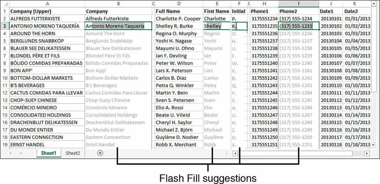
Figure 1.7 In this composite image, you can see that Excel’s new Flash Fill feature can automatically extract or format data based on a pattern you set.
![]() To learn how to apply a custom date format, see “Customizing Date and Time Formats,” p. 84.
To learn how to apply a custom date format, see “Customizing Date and Time Formats,” p. 84.
Note
For Flash Fill’s automatic suggestions to appear, you must have headings at the top of both the column of original data and the column you are using for the filled data. Also, there must not be any blank columns between the filled column and the original column, and the sample entries you make in the filled column must occur one after the other.
Creating a Series
Instead of using the fill handle to create a series, you can use Excel’s Series command to gain a little more control over the whole process. Follow these steps:
1. Select the first cell you want to use for the series and then enter the starting value. If you want to create a series out of a particular pattern (such as 2, 4, 6, and so on), fill in enough cells to define the pattern.
2. Select the entire range you want to fill.
3. Select Home, Fill, Series. Excel displays the Series dialog box.
4. Either click Rows to create the series in rows, starting from the active cell, or click Columns to create the series in columns.
5. Use the Type group to click the type of series you want. You have the following options:
• Linear—This option finds the next series value by adding the step value (see step 7) to the preceding value in the series.
• Growth—This option finds the next series value by multiplying the preceding value by the step value.
• Date—This option creates a series of dates based on the option you select in the Date Unit group (Day, Weekday, Month, or Year).
• AutoFill—This option works much like the fill handle. You can use it to extend a numeric pattern or a text series (for example, Qtr1, Qtr2, Qtr3).
6. If you want to extend a series trend, activate the Trend check box. You can use this option only with the Linear or Growth series types.
7. If you chose a Linear, Growth, or Date series type, enter a number in the Step Value box. This number is what Excel uses to increment each value in the series.
8. To place a limit on the series, enter the appropriate number in the Stop Value box.
9. Click OK. Excel fills in the series and returns you to the worksheet.
Figure 1.8 shows some sample column series. Note that the Growth series stops at cell C12 (value 128) because the next term in the series (256) is greater than the stop value of 250. The Day series fills the range with every second date (because the step value is 2). The Weekday series is slightly different: The dates are sequential, but weekends are skipped.
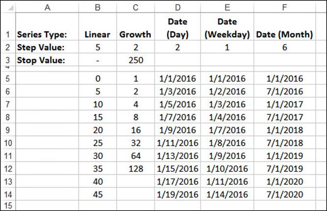
Figure 1.8 Some sample column series generated with the Series command.
Advanced Range Copying and Pasting
The standard Excel range-copying techniques—for example, choosing Home, Copy (or pressing Ctrl+C) and then choosing Home, Paste (or pressing Ctrl+V)—normally copy the entire contents of each cell in the range: the value or formula, the formatting, and any attached cell comments. If you like, you can tell Excel to paste only some of these attributes, you can transpose rows and columns, or you can combine the source and destination ranges arithmetically. All this is possible with Excel’s Paste Special command. These techniques are outlined in the next three sections.
Pasting Selected Cell Attributes
When rearranging a worksheet, you can save time by combining cell attributes. For example, if you need to copy several formulas to a range but don’t want to disturb the existing formatting, you can tell Excel to paste only the formulas.
If you want to paste only selected cell attributes, follow these steps:
1. Select and then copy the range you want to work with.
2. Select the destination range.
3. Select Home, pull down the Paste menu, and then select Paste Special. Excel displays the Paste Special dialog box, shown in Figure 1.9.
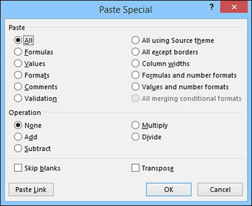
Figure 1.9 Use the Paste Special dialog box to select the cell attributes you want to paste.
Tip
You also can display the Paste Special dialog box by pressing Ctrl+Alt+V or by right-clicking the destination range and choosing Paste Special from the shortcut menu.
4. In the Paste group, click the attribute you want to paste into the destination range:
• All—Pastes all the source range’s cell attributes.
• Formulas—Pastes only the cell formulas. (You can also select Home, Paste, Formulas.)
• Values—Converts the cell formulas to values and pastes only the values. (You can also select Home, Paste, Paste Values.)
• Formats—Pastes only the cell formatting.
• Comments—Pastes only the cell comments.
• Validation—Pastes only the cell-validation rules.
• All Using Source Theme—Pastes all the cell attributes and then formats the copied range using the theme that’s applied to the copied range.
• All Except Borders—Pastes all the cell attributes except the cell’s border formatting. (You can also select Home, Paste, No Borders.)
• Column Widths—Changes the widths of the destination columns to match the widths of the source columns. No data is pasted.
• Formulas and Number Formats—Pastes the cell formulas and numeric formatting.
• Values and Number Formats—Converts the cell formulas to values and pastes only the values and the numeric formats.
• All Merging Conditional Formats—Pastes all the cell attributes and merges the conditional formatting from the source and destination ranges.
5. If you don’t want Excel to paste any blank cells included in the selection, activate the Skip Blanks check box.
6. If you want to paste only formulas that set the destination cells equal to the values of the source cells, click Paste Link. (For example, if the source cell is A1, the value of the destination cell is set to the formula =$A$1.) Otherwise, click OK to paste the range.
Combining Two Ranges Arithmetically
Excel enables you to combine two ranges arithmetically. For example, suppose you have a range of constants that you want to double. Instead of creating formulas that multiply each cell by 2 (or, even worse, doubling each cell by hand), you can place the number 2 in a cell, copy it, and then “paste” it to the range of constants using multiplication.
A more complex example would be a list of prices that you want to increase, but by varying amounts: some by $1, some by $2, some by $0.50, and so on. Again, instead of handling these increases by creating formulas or performing the arithmetic by hand, you can get Excel to do the work. In this case, you’d create a new range of values, each of which represents a price increase for the corresponding original price, so the resulting range would be the same size as the range of original prices. You then combine this new range with the old one and tell Excel to add the two ranges.
The following steps show you what to do:
1. Create the range of values you want to apply to the original range:
• If you want to apply a single value to the original range (for example, multiplying the original values by 2), enter that value in a single cell.
• If you want to apply multiple values to the original range, create a range of values that’s the same size as the original range.
2. Select the range you created in step 1.
3. Select Home, Copy.
4. Select the range of original values.
5. Select Home, click the bottom half of the Paste button, and then select Paste Special to display the Paste Special dialog box.
6. Use the following options in the Operation group to click the arithmetic operator you want to use:
• None—Performs no operation.
• Add—Adds the destination cells to the source cells.
• Subtract—Subtracts the source cells from the destination cells.
• Multiply—Multiplies the source cells by the destination cells.
• Divide—Divides the destination cells by the source cells.
7. If you don’t want Excel to include any blank cells in the operation, activate the Skip Blanks check box.
8. Click OK. Excel pastes the results of the operation into the destination range. Note that the results are the final values, not formulas.
Transposing Rows and Columns
If you have row data that you’d prefer to see in columns (or vice versa), you can use the Transpose command to transpose the data. Follow these steps:
1. Select and copy the source cells.
2. Select the upper-left corner of the destination range.
3. Select Home, pull down the Paste menu, and select Transpose. (If you already have the Paste Special dialog box open, activate the Transpose check box and then click OK.) Excel transposes the source range, as shown in Figure 1.10.
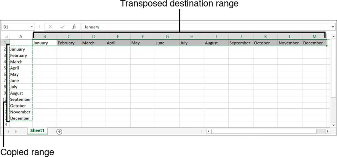
Figure 1.10 You can use the Transpose command to transpose a column of data into a row (as shown here) or vice versa.
Clearing a Range
Deleting a range actually removes the cells from the worksheet. However, if you want the cells to remain, but you want their contents or formats cleared, you can use Excel’s Clear command, as described in the following steps:
1. Select the range you want to clear.
2. Select Home, Clear. Excel displays a submenu of Clear commands.
3. Select Clear All, Clear Formats, Clear Contents, Clear Comments, or Clear Hyperlinks, as appropriate.
To clear the values and formulas in a range with the fill handle, you can use either of the following two techniques:
![]() If you want to clear only the values and formulas in a range, select the range and then click and drag the fill handle into the range and over the cells you want to clear. Excel grays out the cells as you select them. When you release the mouse button, Excel clears the cells’ values and formulas.
If you want to clear only the values and formulas in a range, select the range and then click and drag the fill handle into the range and over the cells you want to clear. Excel grays out the cells as you select them. When you release the mouse button, Excel clears the cells’ values and formulas.
![]() If you want to scrub everything from the range (values, formulas, formats, and comments), select the range and then hold down the Ctrl key. Next, click and drag the fill handle into the range and over each cell you want to clear. Excel clears the cells when you release the mouse button.
If you want to scrub everything from the range (values, formulas, formats, and comments), select the range and then hold down the Ctrl key. Next, click and drag the fill handle into the range and over each cell you want to clear. Excel clears the cells when you release the mouse button.
Applying Conditional Formatting to a Range
Many Excel worksheets contain hundreds of data values. This book is designed to help you make sense of large sets of data by creating formulas, applying functions, and performing data analysis. However, there are plenty of times when you don’t really want to analyze a worksheet per se. Instead, all you really want are answers to simple questions such as the following:
![]() Which cell values are less than 0?
Which cell values are less than 0?
![]() What are the top 10 values?
What are the top 10 values?
![]() Which cell values are above average, and which are below average?
Which cell values are above average, and which are below average?
These simple questions aren’t easy to answer just by glancing at the worksheet, and the more numbers you’re dealing with, the harder it gets. To help you “eyeball” your worksheets and answer these and similar questions, Excel lets you apply conditional formatting to the cells. This is a special format that Excel only applies to cells that satisfy some condition, which Excel calls a rule. For example, you could show all the negative values in a red font.
Creating Highlight Cells Rules
A highlight cell rule is one that applies a format to cells that meet specified criteria. To create a highlight cell rule, begin by choosing Home, Conditional Formatting, Highlight Cells Rules. Excel displays seven choices:
![]() Greater Than—Select this command to apply formatting to cells with values greater than the value you specify. For example, if you want to identify sales reps who increased their sales by more than 10% over last year, you’d create a column that calculates the percentage difference in yearly sales, and you’d then apply the Greater Than rule to that column to look for increases greater than 0.1.
Greater Than—Select this command to apply formatting to cells with values greater than the value you specify. For example, if you want to identify sales reps who increased their sales by more than 10% over last year, you’d create a column that calculates the percentage difference in yearly sales, and you’d then apply the Greater Than rule to that column to look for increases greater than 0.1.
![]() Less Than—Select this command to apply formatting to cells with values less than the value you specify. For example, if you want to recognize divisions, products, or reps whose sales fell from the previous year, you’d use this command to look for percentage or absolute differences that are less than 0.
Less Than—Select this command to apply formatting to cells with values less than the value you specify. For example, if you want to recognize divisions, products, or reps whose sales fell from the previous year, you’d use this command to look for percentage or absolute differences that are less than 0.
![]() Between—Select this command to apply formatting to cells with values between the two values you specify. For example, if you have a series of fixed-income investment possibilities on a worksheet and you’re only interested in medium-term investments, you’d apply this rule to highlight investments where the value in the Term column (expressed in years) is between 5 and 10.
Between—Select this command to apply formatting to cells with values between the two values you specify. For example, if you have a series of fixed-income investment possibilities on a worksheet and you’re only interested in medium-term investments, you’d apply this rule to highlight investments where the value in the Term column (expressed in years) is between 5 and 10.
![]() Equal To—Select this command to apply formatting to cells with values equal to the value you specify. For example, in a table of product inventory where you’re interested in products that are currently out of stock, you’d apply this rule to highlight those products where the value in the On Hand column equals 0.
Equal To—Select this command to apply formatting to cells with values equal to the value you specify. For example, in a table of product inventory where you’re interested in products that are currently out of stock, you’d apply this rule to highlight those products where the value in the On Hand column equals 0.
![]() Text That Contains—Select this command to apply formatting to cells with text values that contain the text value you specify (which is not case sensitive). For example, in a table of bonds that includes ratings where you’re interested only in those bonds that are upper-medium quality or higher (A, AA, or AAA), you’d apply this rule to highlight ratings that include the letter A. (Note that this doesn’t work for certain rating codes that include A in lower ratings, such as Baa and Ba.)
Text That Contains—Select this command to apply formatting to cells with text values that contain the text value you specify (which is not case sensitive). For example, in a table of bonds that includes ratings where you’re interested only in those bonds that are upper-medium quality or higher (A, AA, or AAA), you’d apply this rule to highlight ratings that include the letter A. (Note that this doesn’t work for certain rating codes that include A in lower ratings, such as Baa and Ba.)
![]() A Date Occurring—Select this command to apply formatting to cells with date values that satisfy the condition you select: Yesterday, Today, Tomorrow, In the Last 7 Days, Next Week, and so on. For example, in a table of employee data that includes birthdays, you could apply this command to the birthdays to look for those that occur next week so you can plan celebrations ahead of time.
A Date Occurring—Select this command to apply formatting to cells with date values that satisfy the condition you select: Yesterday, Today, Tomorrow, In the Last 7 Days, Next Week, and so on. For example, in a table of employee data that includes birthdays, you could apply this command to the birthdays to look for those that occur next week so you can plan celebrations ahead of time.
![]() Duplicate Values—Select this command to apply formatting to cells with values that appear more than once in the range. For example, if you have a table of account numbers, no two customers should have the same account number, so you can apply the Duplicate Values rule to those numbers to make sure they’re unique. You can also format cells with unique values—values that appear only once in the range.
Duplicate Values—Select this command to apply formatting to cells with values that appear more than once in the range. For example, if you have a table of account numbers, no two customers should have the same account number, so you can apply the Duplicate Values rule to those numbers to make sure they’re unique. You can also format cells with unique values—values that appear only once in the range.
In each case, you see a dialog box that you use to specify the condition and the formatting that you want applied to cells that match the condition. For example, Figure 1.11 shows the Less Than dialog box. In this case, I’m looking for cell values that are less than 0; Figure 1.12 shows the worksheet with the conditional formatting applied.
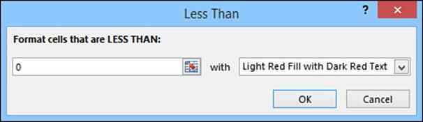
Figure 1.11 In the Highlight Cells Rules menu, select a command to display a dialog box for entering your condition, such as the Less Than dialog box shown here.
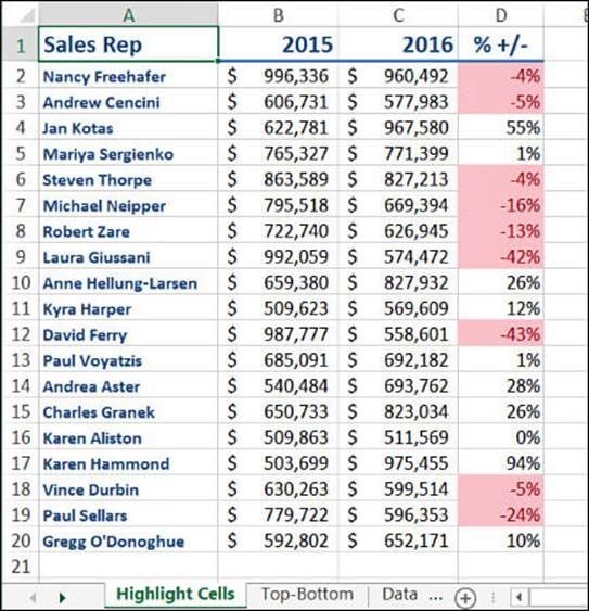
Figure 1.12 The conditional formatting rule shown in Figure 1.11 applied to the percentages in column D.
Creating Top/Bottom Rules
A top/bottom rule is a rule that applies a format to cells that rank in the top or bottom (for numerical items, the highest or lowest) values in a range. You can select the top or bottom either as an absolute value (for example, the top 10 items) or as a percentage (for example, the bottom 25%). You can also apply formatting to cells that are above or below the average. To create a top/bottom rule, begin by choosing Home, Conditional Formatting, Top/Bottom Rules. Excel displays six choices:
![]() Top 10 Items—Select this command to apply formatting to cells with values that rank in the top X items in the range, where X is the number of items you want to see. (The default is 10.) For example, in a table of product sales, you could use this rule to see the top 50 products.
Top 10 Items—Select this command to apply formatting to cells with values that rank in the top X items in the range, where X is the number of items you want to see. (The default is 10.) For example, in a table of product sales, you could use this rule to see the top 50 products.
![]() Top 10%—Select this command to apply formatting to cells with values that rank in the top X percentage of items in the range, where X is the percentage you want to see. (The default is 10.) For example, in a table of sales by sales rep, you could recognize your elite performers by applying this rule to see those reps who are in the top 5%.
Top 10%—Select this command to apply formatting to cells with values that rank in the top X percentage of items in the range, where X is the percentage you want to see. (The default is 10.) For example, in a table of sales by sales rep, you could recognize your elite performers by applying this rule to see those reps who are in the top 5%.
![]() Bottom 10 Items—Select this command to apply formatting to cells with values that rank in the bottom X items in the range, where X is the number of items you want to see. (The default is 10.) For example, if you have a table of unit sales by product, you could apply this rule to see the 20 products that sold the fewest units with an eye to either promoting those products or discontinuing them.
Bottom 10 Items—Select this command to apply formatting to cells with values that rank in the bottom X items in the range, where X is the number of items you want to see. (The default is 10.) For example, if you have a table of unit sales by product, you could apply this rule to see the 20 products that sold the fewest units with an eye to either promoting those products or discontinuing them.
![]() Bottom 10%—Select this command to apply formatting to those cells with values that rank in the bottom X percentage of items in the range, where X is the percentage you want to see. (The default is 10.) For example, in a table that displays product manufacturing defects, you could apply this rule to see those products that rank in the bottom 10% and so are the most reliably produced.
Bottom 10%—Select this command to apply formatting to those cells with values that rank in the bottom X percentage of items in the range, where X is the percentage you want to see. (The default is 10.) For example, in a table that displays product manufacturing defects, you could apply this rule to see those products that rank in the bottom 10% and so are the most reliably produced.
![]() Above Average—Select this command to apply formatting to those cells with values that are above the average of all the values in the range. For example, in a table of investment returns, you could apply this rule to see those investments that are performing above the average for all your investments.
Above Average—Select this command to apply formatting to those cells with values that are above the average of all the values in the range. For example, in a table of investment returns, you could apply this rule to see those investments that are performing above the average for all your investments.
![]() Below Average—Select this command to apply formatting to those cells with values that are below the average of all the values in the range. For example, if you have a list of products and the margins they generate, you could apply this rule to see those that have below-average margins so that you can take steps to improve sales or reduce costs.
Below Average—Select this command to apply formatting to those cells with values that are below the average of all the values in the range. For example, if you have a list of products and the margins they generate, you could apply this rule to see those that have below-average margins so that you can take steps to improve sales or reduce costs.
In each case, you see a dialog box that you use to set up the specifics of the rule. For the Top 10 Items, Top 10%, Bottom 10 Items, and Bottom 10% rules, you use the dialog box to specify the condition and the formatting you want applied to cells that match the condition. (For the Above Average and Below Average rules, you use the dialog box to specify the formatting only.) For example, Figure 1.13 shows the Top 10 Items dialog box. In this case, I’m looking for the top 10 values in the range; Figure 1.14 shows the worksheet with the conditional formatting applied.
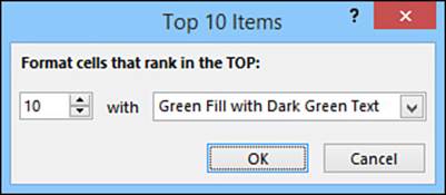
Figure 1.13 In the Top/Bottom Rules menu, select a command to display a dialog box for entering your condition, such as the Top 10 Items dialog box shown here.
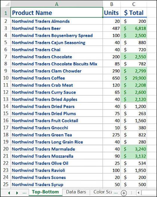
Figure 1.14 The conditional formatting rule shown in Figure 1.13 applied to the dollar values in column C.
Caution
Excel supports unlimited (within the confines of your system memory) conditional formatting rules for any range. Be careful, though: When you apply a rule, select the range, and then apply another rule, Excel does not replace the original rule. Instead, it adds the new rule to the existing one. If you want to change an existing rule, select Home, Conditional Formatting, Manage Rules, click the rule, and then click Edit Rule.
Adding Data Bars
Applying formatting to cells based on highlight cells rules or top/bottom rules is a great way to get particular values to stand out in a crowded worksheet. However, what if you’re more interested in the relationship between similar values in a worksheet? For example, if you have a table of products that includes a column showing unit sales, how do you compare the relative sales of all the products? You could create a new column that calculates the percentage of unit sales for each product relative to the highest value. If the product with the highest sales sold 1,000 units, a product that sold 500 units will show 50% in the new column.
That would work, but all you’re doing is adding more numbers to the worksheet, which might not make things any clearer. You really need some way to visualize the relative values in a range, and that’s where Excel’s data bars come in. Data bars are colored, horizontal bars that appear “behind” the values in a range. (They’re reminiscent of a bar chart.) Their key feature is that the length of the data bar that appears in each cell depends on the value in that cell: The larger the value, the longer the data bar. The cell with the highest value has the longest data bar, and the data bars that appear in the other cells have lengths that reflect their values. (For example, a cell with a value that is half of the largest value would have a data bar that’s half as long as the longest data bar.)
To apply data bars to the selected range, select Home, Conditional Formatting, Data Bars and then select the color you prefer. Figure 1.15 shows data bars applied to the values in the worksheet’s Units column.
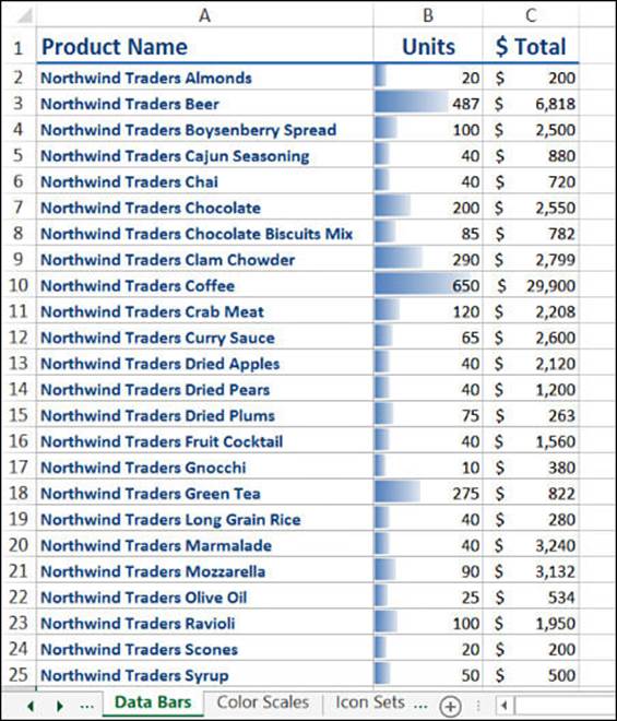
Figure 1.15 Use data bars to visualize the relative values in a range.
Excel configures its default data bars with the longest data bar based on the highest value in the range, and the shortest data bar based on the lowest value in the range. However, what if you want to visualize your values based on different criteria? With test scores, for example, you might prefer to see the data bars based on values between 0 and 100 (so for a value of 50, the data bar always fills only half the cell, no matter what the top mark is).
To apply custom data bars, select the range and then select Home, Conditional Formatting, Data Bars, More Rules to display the New Formatting Rule dialog box, shown in Figure 1.16. In the Edit the Rule Description group, make sure Data Bar appears in the Format Style list. Notice that there’s a Type list for both Minimum and Maximum. The type determines how Excel applies the data bars. You have six choices:
![]() Automatic—This is the default choice, and it means that Excel selects the type automatically, based on the data.
Automatic—This is the default choice, and it means that Excel selects the type automatically, based on the data.
![]() Lowest/Highest Value—With this bar type, the lowest value in the range gets the shortest data bar, and the highest value in the range gets the longest data bar. This is the most common type, and it’s the type Excel usually selects when you have the Type list values set to Automatic.
Lowest/Highest Value—With this bar type, the lowest value in the range gets the shortest data bar, and the highest value in the range gets the longest data bar. This is the most common type, and it’s the type Excel usually selects when you have the Type list values set to Automatic.
![]() Number—Use this type to base the data bar lengths on values that you specify in the two Value text boxes. For Shortest Bar, any cell in the range that has a value less than or equal to the value you specify will get the shortest data bar; similarly, for Longest Bar, any cell in the range that has a value greater than or equal to the value you specify will get the longest data bar.
Number—Use this type to base the data bar lengths on values that you specify in the two Value text boxes. For Shortest Bar, any cell in the range that has a value less than or equal to the value you specify will get the shortest data bar; similarly, for Longest Bar, any cell in the range that has a value greater than or equal to the value you specify will get the longest data bar.
![]() Percent—Use this type to base the data bar lengths on a percentage of the largest value in the range. For Shortest Bar, any cell in the range that has a relative value less than or equal to the percentage you specify will get the shortest data bar; for example, if you specify 10% and the largest value in the range is 1,000, any cell with a value of 100 or less will get the shortest data bar. For Longest Bar, any cell in the range that has a relative value greater than or equal to the percentage you specify will get the longest data bar; for example, if you specify 90% and the largest value in the range is 1,000, any cell with a value of 900 or more will get the longest data bar.
Percent—Use this type to base the data bar lengths on a percentage of the largest value in the range. For Shortest Bar, any cell in the range that has a relative value less than or equal to the percentage you specify will get the shortest data bar; for example, if you specify 10% and the largest value in the range is 1,000, any cell with a value of 100 or less will get the shortest data bar. For Longest Bar, any cell in the range that has a relative value greater than or equal to the percentage you specify will get the longest data bar; for example, if you specify 90% and the largest value in the range is 1,000, any cell with a value of 900 or more will get the longest data bar.
![]() Formula—Use this type to base the data bar lengths on a formula. I discuss this type in Chapter 8, “Working with Logical and Information Functions.”
Formula—Use this type to base the data bar lengths on a formula. I discuss this type in Chapter 8, “Working with Logical and Information Functions.”
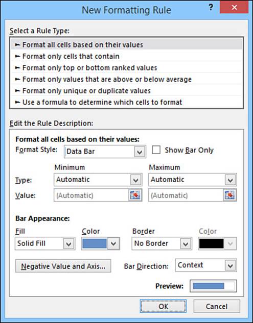
Figure 1.16 Use the New Formatting Rule dialog box to apply a different type of data bar.
![]() To learn how to use the Formula type, see “Applying Conditional Formatting with Formulas,” p. 171.
To learn how to use the Formula type, see “Applying Conditional Formatting with Formulas,” p. 171.
![]() Percentile—Use this type to base the data bar lengths on the percentile within which each cell value falls, given the overall range of the values. In this case, Excel ranks all the values in the range and assigns each cell a position within the ranking. For Shortest Bar, any cell in the range that has a rank less than or equal to the percentile you specify will get the shortest data bar; for example, if you have 100 values and specify the 10th percentile, the cells ranked 10th or less will get the shortest data bar. For Longest Bar, any cell in the range that has a rank greater than or equal to the percentile you specify will get the longest data bar; for example, if you have 100 values and specify the 75th percentile, any cell ranked 75th or higher will get the longest data bar.
Percentile—Use this type to base the data bar lengths on the percentile within which each cell value falls, given the overall range of the values. In this case, Excel ranks all the values in the range and assigns each cell a position within the ranking. For Shortest Bar, any cell in the range that has a rank less than or equal to the percentile you specify will get the shortest data bar; for example, if you have 100 values and specify the 10th percentile, the cells ranked 10th or less will get the shortest data bar. For Longest Bar, any cell in the range that has a rank greater than or equal to the percentile you specify will get the longest data bar; for example, if you have 100 values and specify the 75th percentile, any cell ranked 75th or higher will get the longest data bar.
Adding Color Scales
When examining your data, it’s often useful to get more of a “big picture” view. For example, you might want to know something about the overall distribution of the values. Are there lots of low values and just a few high values? Are most of the values clustered around the average? Are there any outliers, values that are much higher or lower than all or most of the other values? Similarly, you might want to make value judgments about your data. High sales and low numbers of product defects are “good,” whereas low margins and high employee turnover rates are “bad.”
You can analyze your worksheet data in these and similar ways by using Excel’s color scales. A color scale is similar to a data bar in that it compares the relative values of cells in a range. Instead of bars in each cell, though, you see cell shading, where the shading color reflects the cell’s value. For example, the lowest values might be shaded red, the higher values might be shaded light red, then orange, yellow, lime green, and finally deep green for the highest values. The distribution of the colors in the range gives you an immediate visualization of the distribution of the cell values, and outliers jump out because they have a completely different shading from the rest of the range. Value judgments are built in because (in this case) you can think of red as being “bad” (think of a red light) and green as being “good” (a green light).
To apply a color scale, select a range, select Home, Conditional Formatting, Color Scales, and then select the colors. Figure 1.17 shows color scales applied to a range of gross domestic product (GDP) growth rates for various countries.
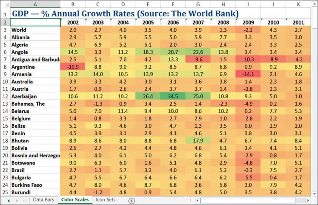
Figure 1.17 Use color scales to visualize the distribution of values in a range.
Your configuration options for color scales are similar to those you learned about in the previous section for data bars. To apply a custom color scale, select the range and then select Home, Conditional Formatting, Color Scales, More Rules to display the New Formatting Rule dialog box. In the Edit the Rule Description group, you can select either 2-Color Scale or 3-Color Scale in the Format Style list. If you select 3-Color Scale, you can select Type, Value, and Color for three parameters Minimum, Midpoint, and Maximum, as shown in Figure 1.18. Note that the items in the Type lists are the same as the ones I discussed for data bars in the previous section.
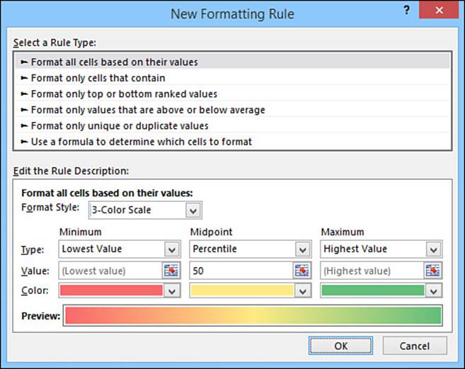
Figure 1.18 Select 3-Color Scale in the Format Style list to apply three colors to your cells.
Adding Icon Sets
When you’re trying to make sense of a great deal of data, symbols are often a useful aid for cutting through the clutter. With movie reviews, for example, a simple thumbs-up (or thumbs-down) is immediately comprehensible and tells something useful about the movie. There are many such symbols that people have strong associations with. For example, a check mark means something is good or finished or acceptable, whereas an X means something is bad or unfinished or unacceptable; a green circle is positive, whereas a red circle is negative (think traffic lights); a smiley face is good, whereas a sad face is bad; an up arrow means things are progressing, a down arrow means things are going backward, and a horizontal arrow means things are remaining as they are.
Excel puts these and many other symbolic associations to good use with the icon sets feature. As with data bars and color scales, you use icon sets to visualize the relative values of cells in a range. In this case, however, Excel adds a particular icon to each cell in the range, and that icon tells you something about the cell’s value relative to the rest of the range. For example, the highest values might get an upward-pointing arrow, the lowest values a downward-pointing arrow, and the values in between a horizontal arrow.
To apply an icon set to the selected range, select Home, Conditional Formatting, Icon Sets and then select the set you want. Figure 1.19 shows the 5 Arrows icon set applied to the percentage increases and decreases in employee sales.
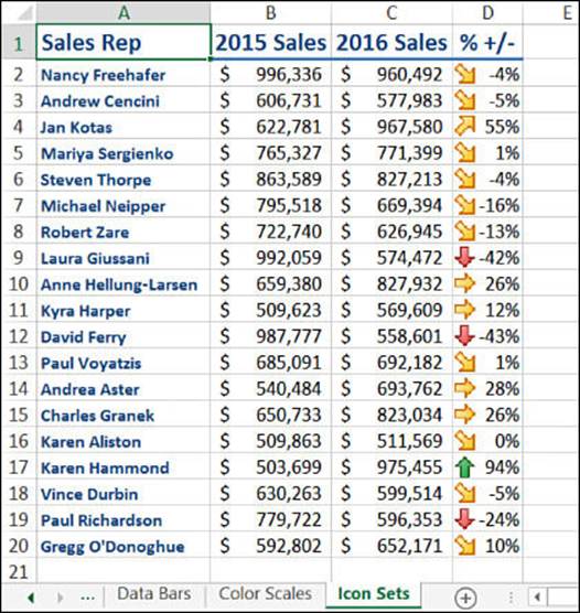
Figure 1.19 Use icon sets to visualize relative values with meaningful symbols.
Your configuration options for icon sets are similar to those you learned about for data bars and color scales. In this case, you need to specify a type and value for each icon (although the range for the lowest icon is always assumed to be less than the lower bound of the second-lowest icon range). To apply a custom icon set, select the range and then select Home, Conditional Formatting, Icon Sets, More Rules to display the New Formatting Rule dialog box, as shown in Figure 1.20. In the Edit the Rule Description group, select the icon set you want in the Icon Style list. Then select an operator, a value, and a type for each icon.
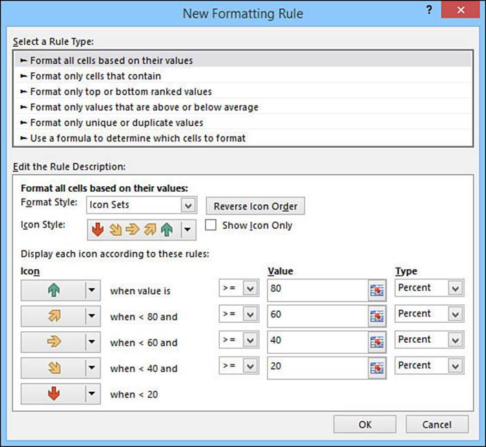
Figure 1.20 The New Formatting Rule dialog box for a custom icon set.
From Here
![]() For information on relative references, see “Understanding Relative Reference Format,” p. 62.
For information on relative references, see “Understanding Relative Reference Format,” p. 62.
![]() For an in-depth discussion of Excel arrays, see “Working with Arrays,” p. 87.
For an in-depth discussion of Excel arrays, see “Working with Arrays,” p. 87.
![]() To learn about data validation, see “Applying Data-Validation Rules to Cells,” p. 100.
To learn about data validation, see “Applying Data-Validation Rules to Cells,” p. 100.
![]() If you’re not sure what a circular reference is, see “Fixing Circular References,” p. 118.
If you’re not sure what a circular reference is, see “Fixing Circular References,” p. 118.
![]() To learn how to create formula-based rules, see “Applying Conditional Formatting with Formulas,” p. 171.
To learn how to create formula-based rules, see “Applying Conditional Formatting with Formulas,” p. 171.
![]() To learn more about using Excel for trend analysis, see “Using Regression to Track Trends and Make Forecasts,” p. 371.
To learn more about using Excel for trend analysis, see “Using Regression to Track Trends and Make Forecasts,” p. 371.
All materials on the site are licensed Creative Commons Attribution-Sharealike 3.0 Unported CC BY-SA 3.0 & GNU Free Documentation License (GFDL)
If you are the copyright holder of any material contained on our site and intend to remove it, please contact our site administrator for approval.
© 2016-2026 All site design rights belong to S.Y.A.