Excel® 2016 Formulas and Functions (2016)
Part I: Mastering Excel Ranges and Formulas
2. Using Range Names
In This Chapter
Defining a Range Name
Working with Range Names
Although ranges enable you to work efficiently with large groups of cells, there are some disadvantages to using range coordinates:
![]() Each time you want to use a range, you must check to see whether it still has the same coordinates (for example, one or more cells might have been inserted or deleted) and, if not, redefine its coordinates.
Each time you want to use a range, you must check to see whether it still has the same coordinates (for example, one or more cells might have been inserted or deleted) and, if not, redefine its coordinates.
![]() Range notation is not intuitive. To know what a formula such as =SUM(E6:E10) is adding, you have to look at the range itself.
Range notation is not intuitive. To know what a formula such as =SUM(E6:E10) is adding, you have to look at the range itself.
![]() A slight mistake in defining the range coordinates can lead to disastrous results, especially when you’re erasing a range.
A slight mistake in defining the range coordinates can lead to disastrous results, especially when you’re erasing a range.
You can overcome these problems by using range names, which are labels applied to a single cell or to a range of cells. You can use a defined name in place of the range coordinates. For example, to include the range in a formula or range command, you use the name instead of selecting the range or typing in its coordinates. You can create as many range names as you like, and you can even assign multiple names to the same range.
Range names also make your formulas intuitive and easy to read. For example, assigning the name AugustSales to a range such as E6:E10 immediately clarifies the purpose of a formula such as =SUM(AugustSales). Range names also increase the accuracy of your range operations because you don’t have to specify range coordinates.
Besides overcoming these problems, range names bring several other advantages to the table:
![]() Names are easier to remember than range coordinates.
Names are easier to remember than range coordinates.
![]() Names don’t change when you move a range to another part of the worksheet.
Names don’t change when you move a range to another part of the worksheet.
![]() Named ranges adjust automatically whenever you insert or delete rows or columns within the range.
Named ranges adjust automatically whenever you insert or delete rows or columns within the range.
![]() Names make it easier to navigate a worksheet. You can use the Go To command to jump to a named range quickly.
Names make it easier to navigate a worksheet. You can use the Go To command to jump to a named range quickly.
![]() You can use worksheet labels to create range names quickly.
You can use worksheet labels to create range names quickly.
In this chapter, I will show you how to define and work with range names, and I also hope to show you the power and flexibility that range names bring to your worksheet chores.
Defining a Range Name
Range names can be quite flexible, but you need to keep in mind a few restrictions and guidelines:
![]() The name can be a maximum of 255 characters.
The name can be a maximum of 255 characters.
![]() The name must begin with either a letter or the underscore character (_). For the rest of the name, you can use any combination of characters, numbers, or symbols (except spaces). For multiple-word names, separate the words by using the underscore character or by mixing case (for example, Cost_Of_Goods or CostOfGoods). Excel doesn’t distinguish between uppercase and lowercase letters in range names.
The name must begin with either a letter or the underscore character (_). For the rest of the name, you can use any combination of characters, numbers, or symbols (except spaces). For multiple-word names, separate the words by using the underscore character or by mixing case (for example, Cost_Of_Goods or CostOfGoods). Excel doesn’t distinguish between uppercase and lowercase letters in range names.
![]() Don’t use cell addresses (such as Q1) or any of the operator symbols (such as +, -, *, /, <, >, and &) because these can cause confusion if you use the name in a formula.
Don’t use cell addresses (such as Q1) or any of the operator symbols (such as +, -, *, /, <, >, and &) because these can cause confusion if you use the name in a formula.
![]() Range names that begin with R or C followed by one or more numbers are illegal because of conflicts with Excel’s R1C1 reference style, where each cell is referenced by its row number followed by its column number (such as R1C1 or R8C2).
Range names that begin with R or C followed by one or more numbers are illegal because of conflicts with Excel’s R1C1 reference style, where each cell is referenced by its row number followed by its column number (such as R1C1 or R8C2).
![]() To make typing easier, try to keep names as short as possible while still keeping them meaningful. TotalProfit2016 is faster to type than Total_Profit_For_Fiscal_Year_2016, and it’s certainly clearer than the more cryptic TotPft16.
To make typing easier, try to keep names as short as possible while still keeping them meaningful. TotalProfit2016 is faster to type than Total_Profit_For_Fiscal_Year_2016, and it’s certainly clearer than the more cryptic TotPft16.
![]() Don’t use any of Excel’s built-in names: Auto_Activate, Auto_Close, Auto_Deactivate, Auto_Open, Consolidate_Area, Criteria, Data_Form, Database, Extract, FilterDatabase, Print_Area, Print_Titles, Recorder, and Sheet_Title.
Don’t use any of Excel’s built-in names: Auto_Activate, Auto_Close, Auto_Deactivate, Auto_Open, Consolidate_Area, Criteria, Data_Form, Database, Extract, FilterDatabase, Print_Area, Print_Titles, Recorder, and Sheet_Title.
With these guidelines in mind, the next few sections show you various methods for defining range names.
Working with the Name Box
The Name box in Excel’s formula bar usually shows just the address of the active cell. However, the Name box also comes with a couple extra features that make it easier to work with range names:
![]() After you’ve defined a name, it appears in the Name box whenever you select the range, as shown in Figure 2.1.
After you’ve defined a name, it appears in the Name box whenever you select the range, as shown in Figure 2.1.
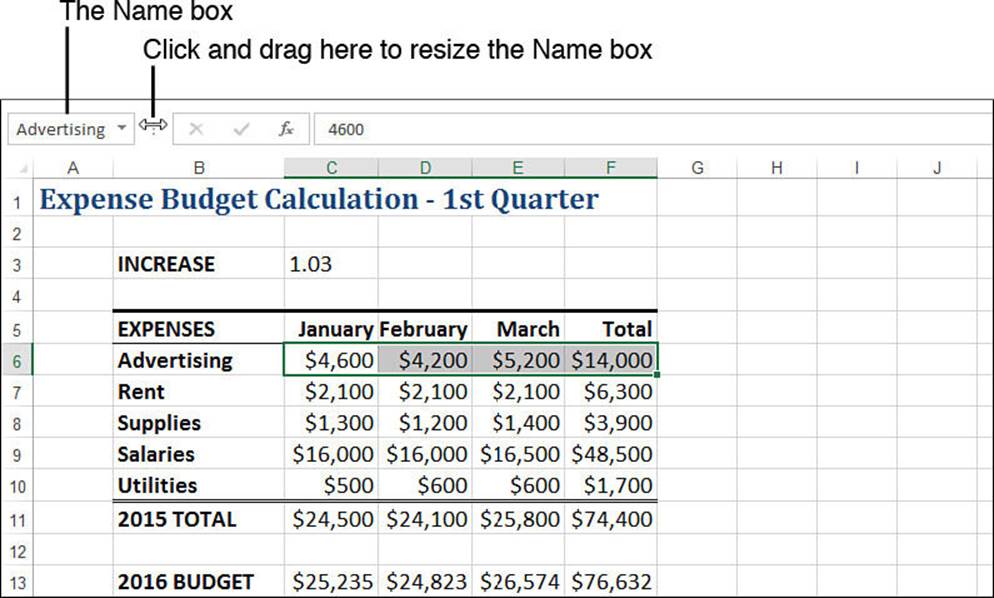
Figure 2.1 When you select a range with a defined name, the name appears in Excel’s Name box.
![]() The Name box doubles as a drop-down list. To select a named range quickly, drop the list down and select the name you want. Excel moves to the range and selects the cells.
The Name box doubles as a drop-down list. To select a named range quickly, drop the list down and select the name you want. Excel moves to the range and selects the cells.
Note
You can download this chapter’s sample workbooks at www.mcfedries.com/books/book.php?title=excel-2016-formulas-and-functions.
One handy feature of the Name box is that it’s resizable. If you can’t see all of the current name, move the mouse cursor to the right edge of the Name box. After it turns into a horizontal, two-headed arrow (see Figure 2.1), click and drag the edge to resize the box.
Using the Name box also happens to be the easiest way to define a range name. Here’s what you do:
1. Select the range you want to name.
2. Click inside the Name box to display the insertion point.
3. Type the name you want to use and then press Enter. Excel defines the new name automatically. (If the range name you typed already exists, Excel selects the range instead of defining a new range name.)
Using the New Name Dialog Box
Using the Name box to define a range name is fast and intuitive, but Excel has other range-naming options available, such as defining the scope of the name and adding a comment for the name. To access these options, follow these steps to define a range name using the New Name dialog box:
1. Select the range you want to name.
2. Select Formulas, Define Name. (Alternatively, right-click the selection and then click Define Name.) The New Name dialog box appears, as shown in Figure 2.2.
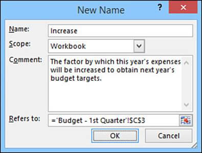
Figure 2.2 When you display the New Name dialog box to define a range name, the coordinates of the selected range appear automatically in the Refers To box.
3. Enter the range name in the Name text box.
Tip
When defining a range name, always enter at least the first letter of the name in uppercase. Why? This will prove invaluable later, when you need to troubleshoot your formulas. The idea is that you type the range name entirely in lowercase letters when you insert it into a formula. When you accept the formula, Excel converts the name to the case you used when you first defined the range name. If the name remains in lowercase letters, you can tell that Excel doesn’t recognize the name, so it’s likely that you misspelled the name when typing it.
4. Use the Scope list to select where you want the name to be available. In most cases, you want to select Workbook, but in the next section I talk about the advantages of limiting the name to a worksheet (see “Changing the Scope to Define Sheet-Level Names”).
5. Use the Comment text box to enter a description or other notes about the range name. This text appears when you use the name in a formula; see “Working with AutoComplete for Range Names,” later in this chapter.
6. If the range displayed in the Refers To box is incorrect, you can use one of two methods to change it:
• Type the correct range address (being sure to begin the address with an equal sign).
• Click inside the Refers To box and then use the mouse or keyboard to select a new range on the worksheet.
Caution
If you need to move around inside the Refers To box with the arrow keys (say, to edit the existing range address), first press F2 to put Excel into Edit mode. If you don’t, Excel remains in Point mode, and the program assumes that you’re trying to select a cell on the worksheet.
7. Click OK to return to the worksheet.
Changing the Scope to Define Sheet-Level Names
Excel enables you to define the scope of a range name. The scope tells you the extent to which the range name will be recognized in formulas. In the New Name dialog box, if you select Workbook from the Scope list (or if you create the name directly using the Name box), the range name is available to all the sheets in a workbook (and is called a workbook-level name). This means, for example, that a formula in Sheet1 can refer to a named range in Sheet3 by using the name directly. This can be a problem, however, if you need to use the same name in different worksheets. For example, say that you have four sheets—First Quarter, Second Quarter, Third Quarter, and Fourth Quarter—and you need to define an Expenses range name in each sheet.
If you need to use the same name in different sheets, you can create a name where the scope is defined for a specific worksheet (and so is called a sheet-level name). This means that the name will refer only to the range on the sheet in which it was defined.
You create a sheet-level name by displaying the New Name dialog box and then using the Scope list to select the worksheet you want to use.
Using Worksheet Text to Define Names
When you use the New Name dialog box, Excel sometimes suggests a name for the selected range. For example, Figure 2.3 shows that Excel has suggested the name Advertising for the range C6:F6. As you can see, Advertising is the row heading of the selected range, so Excel has used an adjacent text entry to make an educated guess about what you want to use as a name.
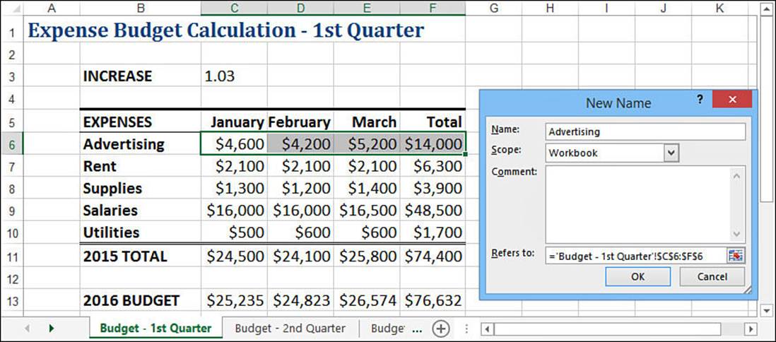
Figure 2.3 Excel often uses adjacent text to guess the range name you want to use.
Instead of waiting for Excel to guess (particularly since Excel sometimes refuses to guess, for reasons unknown), you can tell the program explicitly to use adjacent text as a range name. The following procedure shows you the appropriate steps:
1. Select the range of cells you want to name, including the appropriate text cells you want to use as the range names (see Figure 2.4).
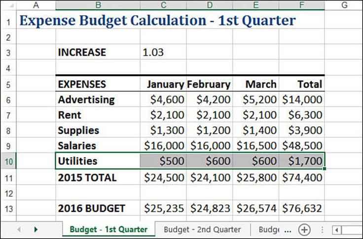
Figure 2.4 Include the text you want to use as the name when you select the range.
2. Select Formulas, Create from Selection or press Ctrl+Shift+F3. Excel displays the Create Names from Selection dialog box, shown in Figure 2.5. Excel guesses where the text for the range name is located and activates the appropriate check box (Left Column, in this example).
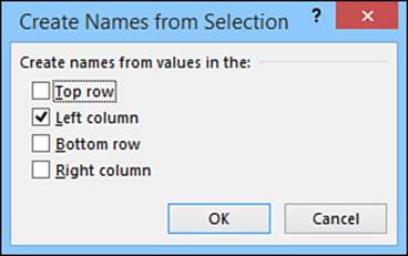
Figure 2.5 Use the Create Names from Selection dialog box to specify the location of the text to use as a range name.
3. If Excel hasn’t correctly guessed about the check box you want, clear it and then activate the appropriate one.
4. Click OK.
Note
If the text you want to use as a range name contains any illegal characters (such as a space), Excel replaces those characters with an underscore (_).
When naming ranges from text, you’re not restricted to working with just columns or rows. Instead, you can select ranges that include both row and column headings, and Excel will happily assign names to each row and column. For example, in Figure 2.6, the Create Names from Selection dialog box appears with both the Top Row and Left Column check boxes selected.
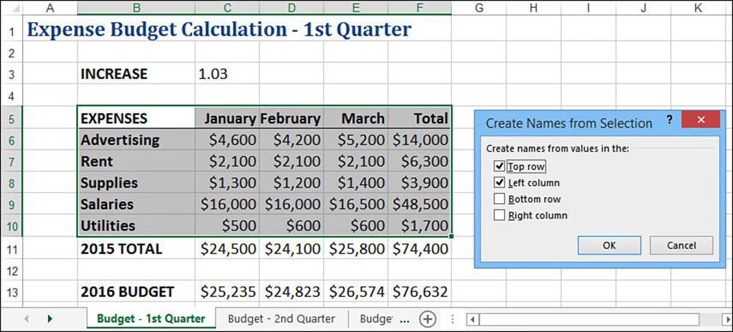
Figure 2.6 Excel can create names for rows and columns at the same time.
When you use this method to create names automatically, bear in mind that Excel gives special treatment to the top-left cell in the selected range. Specifically, it uses the text in that cell as the name for the range that includes the table data (that is, the table without the headings). In Figure 2.6, for example, the upper-left corner of the selected range is cell B5, which contains the label Expenses. After the names have been created, the table data—the range C6:F10—is given the name Expenses, as shown in Figure 2.7. If the top-left cell in the range is blank, Excel doesn’t create a range name for the table.
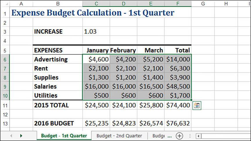
Figure 2.7 When creating names from rows and columns at the same time, Excel uses the label in the top-left corner as the name of the range that includes the table data.
Naming Constants
One of the best ways to make your worksheets comprehensible is to define names for every constant value. For example, if your worksheet uses an interest rate variable in several formulas, you can define a constant named Rate and use this name in your formulas to make them more readable. You can do this in two ways:
![]() Set aside an area of your worksheet for constants and name the individual cells. For example, Figure 2.8 shows a worksheet with three named constants: Rate (cell B5), Term (cell B6), and Amount (cell B7). Notice how the formula in cell E5 refers to each constant by name.
Set aside an area of your worksheet for constants and name the individual cells. For example, Figure 2.8 shows a worksheet with three named constants: Rate (cell B5), Term (cell B6), and Amount (cell B7). Notice how the formula in cell E5 refers to each constant by name.
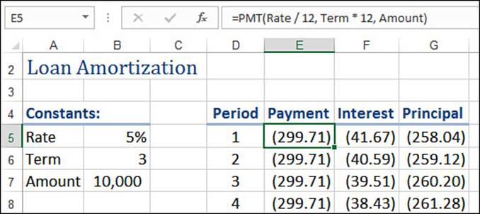
Figure 2.8 Grouping formula constants and naming them makes worksheets easy to read.
![]() If you don’t want to clutter a worksheet, you can name constants without entering them in the worksheet. Select Formulas, Define Name to display the New Name dialog box. Enter a name for the constant in the Name text box and the constant’s value in the Refers To text box. Figure 2.9 shows an example.
If you don’t want to clutter a worksheet, you can name constants without entering them in the worksheet. Select Formulas, Define Name to display the New Name dialog box. Enter a name for the constant in the Name text box and the constant’s value in the Refers To text box. Figure 2.9 shows an example.
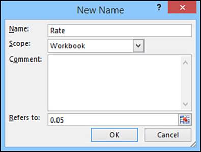
Figure 2.9 You can create and name constants in the New Name dialog box.
Tip
When naming a constant, you’re not restricted to the usual constant values of numbers and text strings. Excel also allows you to assign a worksheet function to a name. For example, you could enter =YEAR(NOW()) in the Refers To text box to create a name that always returns the current year. However, this feature is better suited to assigning a name to a long and complex formula that you need to use in different places.
Working with Range Names
After you’ve defined a name, you can use it in formulas or functions, navigate with it, edit it, and delete it. The next few sections take you through these techniques and more.
Tip
After you’ve defined several range names on a worksheet, it often becomes difficult to visualize the location and dimensions of the ranges. Excel’s Zoom feature can help. Select View, Zoom to display the Zoom dialog box. In the Custom text box, enter a value of 39% or less and then click OK. Excel zooms out and displays the named ranges by drawing a border around each one and displaying the range name centered within the border.
Referring to a Range Name
Using a range name in a formula or as a function argument is straightforward: Just replace a range’s coordinates with the range’s defined name. For example, suppose that a cell contains the following formula:
=G1
This formula sets the cell’s value to the current value of cell G1. However, if cell G1 is named TotalExpenses, the following formula is equivalent:
=TotalExpenses
Similarly, consider the following function:
SUM(E3:E10)
If the range E3:E10 is named Sales, the following is equivalent:
SUM(Sales)
![]() For more information on using names in your Excel formulas, see “Working with Range Names in Formulas,” p. 67.
For more information on using names in your Excel formulas, see “Working with Range Names in Formulas,” p. 67.
If you’re not sure about a particular name, you can get Excel to paste it into the worksheet for you. Here are the steps required:
1. Start your formula or function and stop when you come to the spot where you need to insert the range name.
2. Select Formulas, Use in Formula. Excel displays a list of names whose scope includes the current worksheet, as shown in Figure 2.10.
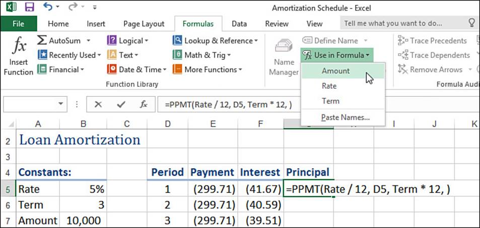
Figure 2.10 Select the Use in Formula command to see a list of defined range names.
3. Click the name you want to use. Excel pastes the name.
If you’re working with sheet-level names, how you use a name depends on where you use it:
![]() If you’re using the sheet-level name on the sheet in which it was defined, you can just use the range name part. (That is, you don’t need to specify the sheet name.)
If you’re using the sheet-level name on the sheet in which it was defined, you can just use the range name part. (That is, you don’t need to specify the sheet name.)
![]() If you’re using the sheet-level name on any other sheet, you must use the full name (SheetName!RangeName).
If you’re using the sheet-level name on any other sheet, you must use the full name (SheetName!RangeName).
If the named range exists in a different workbook, you must precede the name with the name of the file in single quotation marks. For example, if the Mortgage Amortization workbook contains a range named Rate, you use the following in a different workbook to refer to this range:
'Mortgage Amortization.xlsx'!Rate
Caution
Excel doesn’t mind if you create a sheet-level name that’s the same as a workbook-level name. In all the other sheets, if you use the range name by itself, Excel assumes that you’re talking about the workbook-level name. However, if you use only the range name on the sheet in which the sheet-level name was defined, Excel assumes that you’re talking about the sheet-level name.
So how do you refer to the workbook-level name from the sheet in which the sheet-level name was defined? You precede the range name with the workbook filename and an exclamation point. For example, in a workbook named Expenses.xlsx, suppose that the current worksheet has a sheet-level range named Total and that there’s also a workbook-level range named Total. To refer to the latter in the current worksheet, you use the following:
Expenses.xlsx!Total
Working with AutoComplete for Range Names
In Chapter 6, “Understanding Functions,” you’ll see that Excel has an AutoComplete feature that displays a list of function names that match what you’ve typed so far. If you see the function you want, you can select it from the list instead of typing the rest of the function name, which is usually faster and more accurate. Excel offers AutoComplete for range names as well. When you type the first few letters of a range name in a formula, Excel includes the range name as part of the AutoComplete list. As you can see in Figure 2.11, Excel also includes the comment text associated with a range name. To add the name to the formula, use the arrow keys to select it from the list and then press Tab.
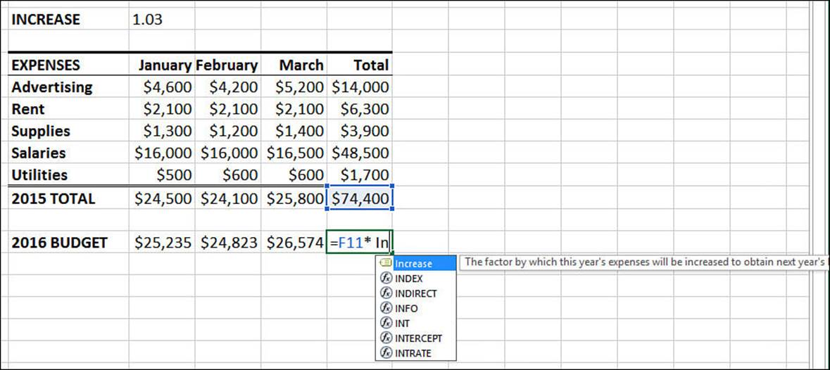
Figure 2.11 Excel offers AutoComplete for range names.
Navigating Using Range Names
Ranges that have defined names are easy to select. Excel gives you two methods:
![]() The Name box doubles as a drop-down list. To select a named range quickly, drop the list down and select the name you want.
The Name box doubles as a drop-down list. To select a named range quickly, drop the list down and select the name you want.
![]() Select Home, Find & Select, Go To (or press F5 or Ctrl+G) to display the Go To dialog box. Click the range name in the Go To list and then click OK.
Select Home, Find & Select, Go To (or press F5 or Ctrl+G) to display the Go To dialog box. Click the range name in the Go To list and then click OK.
Pasting a List of Range Names in a Worksheet
If you need to document a worksheet for others to read (or figure out the worksheet yourself a few months from now), you can paste a list of the worksheet’s range names. This list includes the name and the range it represents (or the value it represents, if the name refers to a constant). It’s a static list (that is, it won’t update if you make changes to the names or ranges), but it gives you a useful overview of the names you’re using in the worksheet. Follow these steps to paste a list of range names:
1. Move to an empty area of the worksheet that’s large enough to accept the list without overwriting any other data. (Note that the list uses up two columns: one for the names and one for the corresponding range coordinates.)
2. Select Formulas, Use in Formula, Paste Names or press F3. Excel displays the Paste Name dialog box.
3. Click Paste List. Excel pastes the worksheet’s names and range coordinates.
Displaying the Name Manager
Excel comes with a Name Manager feature, which is a useful interface for working with range names. To display the Name Manager, select Formulas, Name Manager (or press Ctrl+F3). Figure 2.12 shows the Name Manager dialog box that appears. Note that the columns are resizable (click and drag the right edge of any column’s header) and sortable (click a column’s header to toggle between ascending and descending).
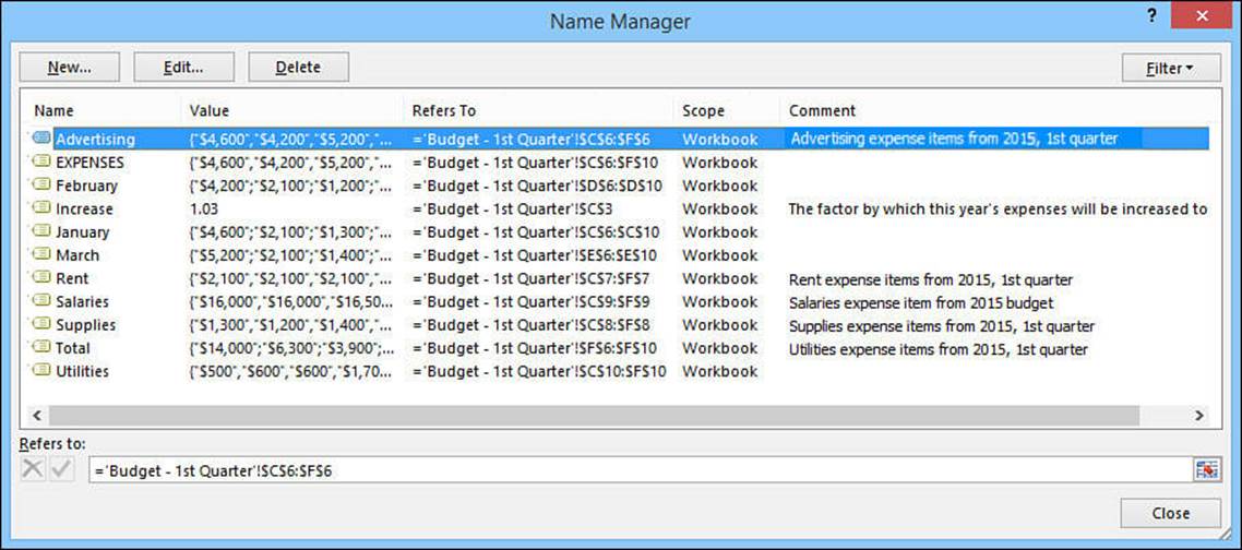
Figure 2.12 Use the Name Manager to modify, filter, or delete range names.
Filtering Names
If you have a workbook with a huge number of defined names, the Name Manager list can become quite unwieldy. To knock it down to size, Excel enables you to filter the display of range names. Click the Filter button and then click one of the following filters:
![]() Clear Filter—Click this item to deactivate all the filters.
Clear Filter—Click this item to deactivate all the filters.
![]() Names Scoped to Worksheet—Activate this filter to see only names that have the current worksheet as their scope.
Names Scoped to Worksheet—Activate this filter to see only names that have the current worksheet as their scope.
![]() Names Scoped to Workbook—Activate this filter to see only names that have the current workbook as their scope.
Names Scoped to Workbook—Activate this filter to see only names that have the current workbook as their scope.
![]() Names with Errors—Activate this filter to see only names that contain an error value, such as #NAME, #REF, or #VALUE.
Names with Errors—Activate this filter to see only names that contain an error value, such as #NAME, #REF, or #VALUE.
![]() Names without Errors—Activate this filter to see only names that don’t contain error values.
Names without Errors—Activate this filter to see only names that don’t contain error values.
![]() Defined Names—Activate this filter to see only names that are built into Excel or that you’ve defined yourself (that is, you don’t see names created automatically by Excel, such as table names).
Defined Names—Activate this filter to see only names that are built into Excel or that you’ve defined yourself (that is, you don’t see names created automatically by Excel, such as table names).
![]() Table Names—Activate this filter to see only names that Excel has generated for tables.
Table Names—Activate this filter to see only names that Excel has generated for tables.
Editing a Range Name’s Coordinates
Sometimes you want an existing name to refer to a different set of range coordinates. Excel offers a couple of ways to edit the name:
![]() Move the range. When you do this, Excel moves the range name right along with it.
Move the range. When you do this, Excel moves the range name right along with it.
![]() If you want to adjust the existing coordinates or associate the name with a completely different range, display the Name Manager, click the name you want to change, and then edit the range coordinates using the Refers To text box.
If you want to adjust the existing coordinates or associate the name with a completely different range, display the Name Manager, click the name you want to change, and then edit the range coordinates using the Refers To text box.
Adjusting Range Name Coordinates Automatically
It’s common in spreadsheet work to have a row or column of data that you add to constantly. For example, you might have to keep a list of ongoing expenses in a project, or you might want to track the number of units of a product that sell each day. From the perspective of range names, this isn’t a problem if you always insert the new data within the existing range. In this case, Excel automatically adjusts the range coordinates to compensate for the new data. However, that doesn’t happen if you always add the new data to the end of the range. In this case, you need to manually adjust the range coordinates to include the new data. The more data you enter, the bigger the pain this can be. To avoid this time-consuming drudgery, this section offers two solutions.
Solution 1: Including a Blank Cell at the End of the Range
The first solution is to define the range and include an extra blank cell at the end, if possible. For example, in the worksheet shown in Figure 2.13, the Amount name has been applied to the range C4:C12, where C12 is a blank cell.
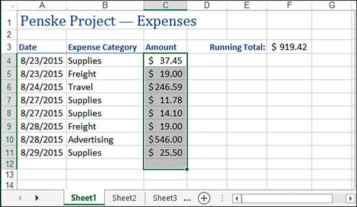
Figure 2.13 To get Excel to adjust a range name’s coordinates automatically, include a blank cell at the end of the range, if possible.
The advantage here is that you can get Excel to adjust the Amount name’s range coordinates automatically by inserting new data above (in this case) the blank row immediately below the table. Because you’re inserting the new data within the existing range, Excel adjusts the name’s range coordinates automatically, as shown in Figure 2.14.
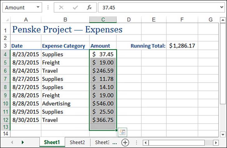
Figure 2.14 The Amount name now refers to the range C4:C13.
Solution 2: Naming the Entire Row or Column
An even easier solution than the one I just showed is to name the entire row or column to which you’re adding data. You do this by selecting the row or column, entering the name in the Name box, and pressing Enter. With this method, any data you add to the row or column automatically becomes part of the range name.
Caution
Use this method only if the row or column to which you’re adding data contains no other conflicting data. For example, if you’re adding numbers to a column and that column has other, unrelated numbers above or below, those numbers will be included in the range name you define for the entire column. This would prevent you from using the name in a formula because the formula would also include the extraneous data.
Changing a Range Name
If you need to change the name of one or more ranges, you can use one of two methods:
![]() If you’ve changed some row or column labels, redefine the range names based on the new text and then delete the old names (as described in the next section).
If you’ve changed some row or column labels, redefine the range names based on the new text and then delete the old names (as described in the next section).
![]() Display the Name Manager, click the name you want to change, and then click Edit to display the Edit Name dialog box. Make your changes in the Name text box and then click OK.
Display the Name Manager, click the name you want to change, and then click Edit to display the Edit Name dialog box. Make your changes in the Name text box and then click OK.
Deleting a Range Name
If you no longer need a range name, you should delete the name from the worksheet to avoid cluttering the name list. The following procedure outlines the necessary steps:
1. Select Formulas, Name Manager.
2. Click the name you want to delete.
3. Click Delete. Excel asks you to confirm the deletion.
4. Click OK.
5. Click Close.
Using Names with the Intersection Operator
With ranges that overlap, you can use the intersection operator (a space) to refer to the overlapping cells. For example, Figure 2.15 shows two ranges: C4:E9 and D8:G11. To refer to the overlapping cells (D8:E9), you use the following notation: C4:E9 D8:G11.
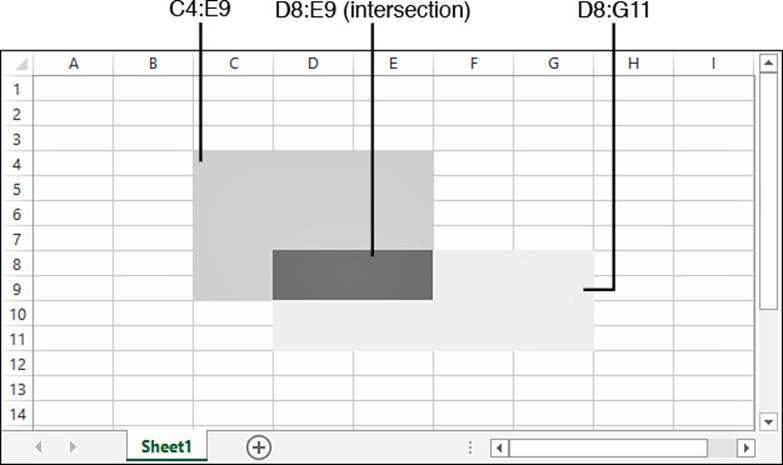
Figure 2.15 The intersection operator returns the intersecting cells of two ranges.
If you’ve named the ranges on your worksheet, the intersection operator can make things much easier to read because you can refer to individual cells by using the names of the cell’s row and column. For example, in Figure 2.16, the range C6:C10 is named January, and the range C7:F7 is named Rent. This means that you can refer to cell C7 as January Rent (see cell I7).
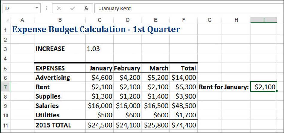
Figure 2.16 After you name ranges, you can combine row and column headings to create intersecting names for individual cells.
Caution
If you try to define an intersection name and Excel displays #NULL! in the cell, it means that the two ranges don’t have any overlapping cells.
From Here
![]() To get the details of Excel’s 3D ranges, see “Working with 3D Ranges,” p. 7.
To get the details of Excel’s 3D ranges, see “Working with 3D Ranges,” p. 7.
![]() For more information on using names in your Excel formulas, see “Working with Range Names in Formulas,” p. 67.
For more information on using names in your Excel formulas, see “Working with Range Names in Formulas,” p. 67.
![]() To learn about AutoComplete for functions, see “Typing a Function into a Formula,” p. 132.
To learn about AutoComplete for functions, see “Typing a Function into a Formula,” p. 132.
All materials on the site are licensed Creative Commons Attribution-Sharealike 3.0 Unported CC BY-SA 3.0 & GNU Free Documentation License (GFDL)
If you are the copyright holder of any material contained on our site and intend to remove it, please contact our site administrator for approval.
© 2016-2026 All site design rights belong to S.Y.A.