Excel® 2016 Formulas and Functions (2016)
Part IV: Building Financial Formulas
20. Building Discount Formulas
In This Chapter
Calculating the Present Value
Discounting Cash Flows
Calculating the Payback Period
Calculating the Internal Rate of Return
In Chapter 19, “Building Investment Formulas,” you saw that investment calculations largely use the same time-value-of-money concepts as the loan calculations that you learned about in Chapter 18, “Building Loan Formulas.” The difference is the direction of the cash flows. For example, the present value of a loan is a positive cash flow because the money comes to you; the present value of an investment is a negative cash flow because the money goes out to the investment.
Discounting also fits into the time-value-of-money scheme, and you can see its relation to present value, future value, and interest earned in the following equations:
Future value = Present value + Interest
Present value = Future value − Discount
In Chapter 18, you learned about a form of discounting when you determined how much money you could borrow (the present value) when you know the current interest rate that your bank offers for loans, when you want to have the loan paid off, and how much you can afford each month for the payments.
![]() See “Calculating How Much You Can Borrow,” p. 446.
See “Calculating How Much You Can Borrow,” p. 446.
Similarly, in Chapter 19, you learned about another application of discounting when you calculated the initial deposit required (the present value) to reach a future goal, knowing how much you can deposit each period and how much the interest rate will be.
![]() See “Calculating the Required Initial Deposit,” p. 461.
See “Calculating the Required Initial Deposit,” p. 461.
This chapter takes a closer look at Excel’s discounting tools, including present value and profitability as well as cash-flow analysis measures such as net present value and internal rate of return.
Calculating the Present Value
The time-value-of-money concept tells you that a dollar now is not the same as a dollar in the future. You can’t compare them directly because it’s like comparing the temporal equivalent of the proverbial apples and oranges. From a discounting perspective, the present value is important because it turns those future oranges into present apples. That is, it enables you to make a true comparison by restating the future value of an asset or investment in today’s terms.
You know from Chapter 19 that calculating a future value relies on compounding. That is, a dollar today grows by applying interest on interest, like this:
Year 1: $1.00 × (1 + rate)
Year 2: $1.00 × (1 + rate) × (1 + rate)
Year 3: $1.00 × (1 + rate) × (1 + rate) × (1 + rate)
![]() See “Understanding Compound Interest,” p. 454.
See “Understanding Compound Interest,” p. 454.
More generally, given an interest rate and a period nper, the future value of a dollar today is calculated as follows:
=$1.00 * (1 + rate) ^ nper
Calculating the present value uses the reverse process. That is, given some discount rate, a future dollar is expressed in today’s dollars by dividing instead of multiplying:
Year 1: $1.00 / (1 + rate)
Year 2: $1.00 / (1 + rate) / (1 + rate)
Year 3: $1.00 / (1 + rate) / (1 + rate) / (1 + rate)
In general, given a discount rate and a period nper, the present value of a future dollar is calculated as follows:
=$1.00 / (1 + rate) ^ nper
The result of this formula is called the discount factor, and multiplying it by any future value restates that value in today’s dollars.
Taking Inflation into Account
The future value tells you how much money you’ll end up with, but it doesn’t tell you how much that money is worth. In other words, if an object costs $10,000 now and your investment’s future value is $10,000, it’s unlikely that you’ll be able to use that future value to purchase the object because it will probably have gone up in price. That is, inflation erodes the purchasing power of any future value; to know what a future value is worth, you need to express it in today’s dollars.
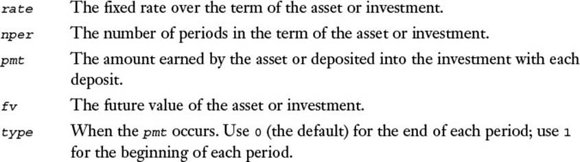
For example, suppose that you put $10,000 initially and $100 per month into an investment that pays 5% annual interest. After 10 years, the future value of that investment will be $31,998.32. Assuming that the inflation rate stays constant at 2% per year, what is the investment’s future value worth in today’s dollars?
Here, the discount rate is the inflation rate, so the discount factor is calculated as follows:
=1 / (1.02) ^ 10
This returns 0.82. Multiplying the future value by this discount factor gives the present value: $26,249.77.
Calculating Present Value Using PV()
You’re probably wondering what happened to Excel’s PV() function. I’ve held off on introducing it so that you could see how to calculate present value from first principles. Now that you know what’s going on behind the scenes, you can make your life easier by calculating present values directly using the PV() function:
PV(rate, nper, pmt[, fv][, type])
For example, to calculate the effect of inflation on a future value, you apply the PV() function to the future value, where the rate argument is the inflation rate:
PV(inflation rate, nper, 0, fv)
Note
When you set the PV() function’s pmt argument to 0, you can ignore the type argument because it’s meaningless without payments.
Figure 20.1 shows a worksheet that uses PV() to derive the answer of $26,249.77 using the following formula:
=PV(B9, B3, 0, -B7)
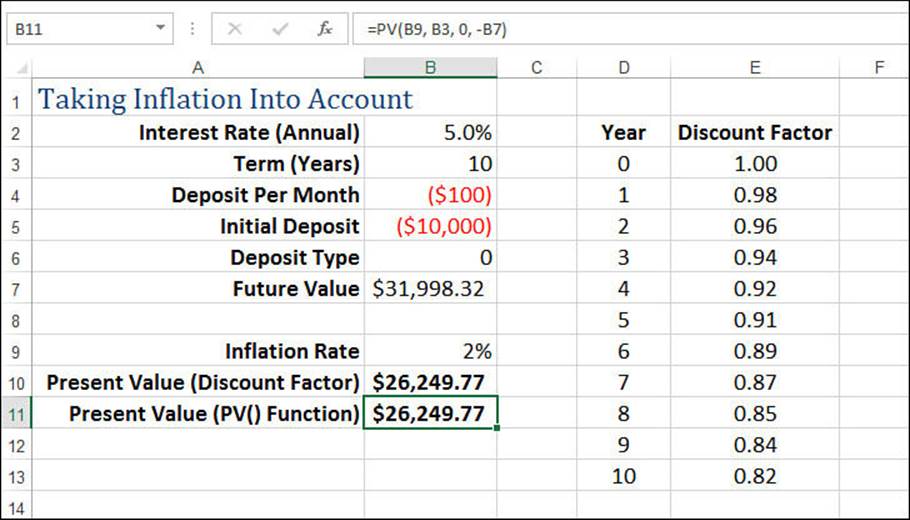
Figure 20.1 Use the PV() function to calculate the effects of inflation on a future value.
Note that this is the same result you derived using the discount factor, which is shown in Figure 20.1 in cell B10. (The table in D2:E13 shows the various discount factors for each year.)
Note
You can download this chapter’s sample workbook at www.mcfedries.com/books/book.php?title=excel-2016-formulas-and-functions.
The next few sections take you through some examples of using PV() in discounting scenarios.
Income Investing Versus Purchasing a Rental Property
If you have some cash to invest, one common scenario is to wonder whether the cash is better invested in a straight income-producing security (such as a bond or certificate) or in a rental property.
One way to analyze this is to gather the following data:
![]() On the fixed-income security side, find your best deal in the time frame you’re looking at. For example, you might find that you can get a bond that matures in 10 years with a 5% yield.
On the fixed-income security side, find your best deal in the time frame you’re looking at. For example, you might find that you can get a bond that matures in 10 years with a 5% yield.
![]() On the rental property side, find out what the property produces in annual rental income. Also, estimate what the rental property will be worth at the same future date that the fixed-income security matures. For example, you might be looking at a rental property that generates $24,000 a year and is estimated to be worth $1 million in 10 years.
On the rental property side, find out what the property produces in annual rental income. Also, estimate what the rental property will be worth at the same future date that the fixed-income security matures. For example, you might be looking at a rental property that generates $24,000 a year and is estimated to be worth $1 million in 10 years.
Given this data (and ignoring complicating factors such as rental property expenses), you want to know the maximum that you should pay for the property to realize a better yield than with the fixed-income security.
To solve this problem, use the PV() function as follows:
=PV(fixed income yield, nper, rental income, future property value)
Figure 20.2 shows a worksheet model that uses this formula. The result of the PV() function is $799,235. You interpret this to mean that if you pay less than that amount for the property, the property is a better deal than the fixed-income security; if you pay more, you’re better off going the fixed-income route.
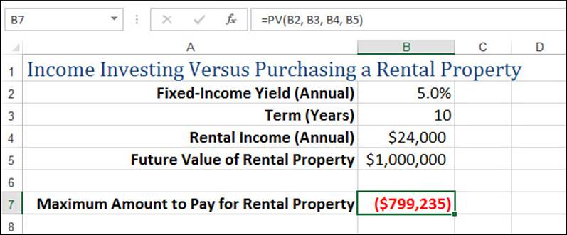
Figure 20.2 Use the PV() function to compare investing in a fixed-income security versus purchasing a rental property.
Buying Versus Leasing
Another common business conundrum is whether to purchase equipment outright or to lease it. Again, you figure the present value of both sides to compare them, with the preferable option being the one that provides the lower present value. (This ignores complicating factors such as depreciation and taxes.)
Assume (for now) that the purchased equipment has no market value at the end of the term and that the leased equipment has no residual value at the end of the lease. In this case, the present value of the purchase option is simply the purchase price. For the lease option, you determine the present value using the following form of the PV() function:
=PV(discount rate, lease term, lease payment)
For the discount rate, you plug in a value that represents either a current investment rate or a current loan rate. For example, if you could invest the lease payment and get 6% per year, you would plug 6% into the function as the rate argument.
Suppose you can either purchase a piece of equipment for $5,000 now or lease the equipment for $240 a month over two years. Assuming a discount rate of 6%, what’s the present value of the leasing option? Figure 20.3 shows a worksheet that calculates the answer: $5,415.09. This means that purchasing the equipment is the less costly choice.
Figure 20.3 Use the PV() function to compare buying versus leasing equipment.
What if the equipment has a future market value (on the purchase side) or a residual value (on the lease side)? This won’t make much difference in terms of which option is better because the future value of the equipment raises the two present values by about the same amount. However, note how you calculate the present value for the purchase option:
=purchase price + PV(discount rate, term, 0, future value)
That is, the present value of the purchase option is the price plus the present value of the equipment’s future market value. (For the lease option, you include the residual value as the PV() function’s fv argument.) Figure 20.4 shows the worksheet with a future value added.
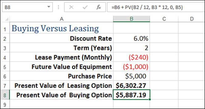
Figure 20.4 Use the PV() function to compare buying versus leasing equipment that has a future market or residual value.
Discounting Cash Flows
One very common business scenario is to put some money into an asset or investment that generates income. By examining the cash flows—the negative cash flows for the original investment and any subsequent outlays required by the asset, and the positive cash flows for the income generated by the asset—you can figure out whether you’ve made a good investment.
For example, consider the situation discussed earlier in this chapter: You invest in a property that generates a regular cash flow of rental income. When analyzing this investment, you have three types of cash flow to consider:
![]() The initial purchase price (negative cash flow)
The initial purchase price (negative cash flow)
![]() The annual rental income (positive cash flow)
The annual rental income (positive cash flow)
![]() The price you get by selling the property (positive cash flow)
The price you get by selling the property (positive cash flow)
Earlier you used the PV() function to calculate that an initial purchase price of $799,235 and an assumed sale price of $1 million gives you the same return as a 5% fixed-income security over 10 years. Let’s verify this using a cash-flow analysis. Figure 20.5 shows a worksheet set up to show the cash flows for this investment. Row 3 shows the net cash flow each year. (In practice, this would be the rental income minus the costs incurred while maintaining and repairing the property.) Row 4 shows the cumulative net cash flows. Note that columns F through I (years 4 through 7) are hidden so that you can see the final cash flow: the rent in year 10 plus the sale price of the property.
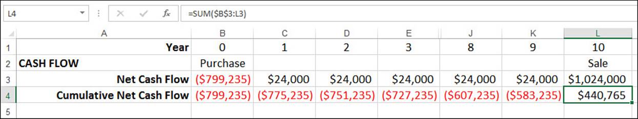
Figure 20.5 The yearly and cumulative cash flows for a rental property.
Calculating the Net Present Value
The net present value is the sum of a series of net cash flows, each of which has been discounted to the present using a fixed discount rate. If all the cash flows are the same, you can use the PV() function to calculate the present value. But when you have a series of varying cash flows, as in the rental property example, you can apply the PV() function directly.
Excel has a direct route to calculating net present value, but let’s take a second to examine a method that calculates this value from first principles. This will help you understand exactly what’s happening in this kind of cash-flow analysis.
To get the net present value, you first have to discount each cash flow. You do that by multiplying the cash flow by the discount factor, which you calculate as described earlier in this chapter.
Figure 20.6 shows the rental property cash-flow worksheet with the discount factors (row 8) and the discounted cash flows (rows 9 and 10).
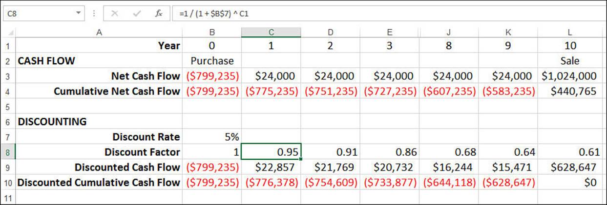
Figure 20.6 The discounted yearly and cumulative cash flows for a rental property.
The key number to notice in Figure 20.6 is the final Discounted Cumulative Cash Flow value in cell L10, which is $0. This is the net present value, the sum of the cumulative discounted cash flows at the end of year 10. This result makes sense because you already know that the initial cash flow—the purchase price of $799,235—was the present value of the rental income with a discount rate of 5% and a sale price of $1 million.
In other words, purchasing the property for $799,235 enables you to break even—that is, the net present value is 0—when all the cash flows are discounted into today’s dollars using the specified discount rate.
Note
The discount rate that returns a net present value of 0 is sometimes called the hurdle rate. In other words, it’s the rate that you must surpass to make the asset or investment worthwhile.
The net present value can also tell you whether an investment is positive or negative:
![]() If the net present value is negative, this can generally be interpreted in two ways: Either you paid too much for the asset or the income from the asset is too low. For example, if you plug −$900,000 into the rental property model as the initial cash flow (that is, the purchase price), the net present value works out to −$100,765, which is the loss on the property in today’s dollars.
If the net present value is negative, this can generally be interpreted in two ways: Either you paid too much for the asset or the income from the asset is too low. For example, if you plug −$900,000 into the rental property model as the initial cash flow (that is, the purchase price), the net present value works out to −$100,765, which is the loss on the property in today’s dollars.
![]() If the net present value is positive, this can generally be interpreted in two ways: Either you got a good deal for the asset or the income makes the asset profitable. For example, if you plug −$700,000 into the rental property model as the initial cash flow (that is, the purchase price), the net present value works out to $99,235, which is the profit on the property in today’s dollars.
If the net present value is positive, this can generally be interpreted in two ways: Either you got a good deal for the asset or the income makes the asset profitable. For example, if you plug −$700,000 into the rental property model as the initial cash flow (that is, the purchase price), the net present value works out to $99,235, which is the profit on the property in today’s dollars.
Calculating Net Present Value Using NPV()
The model built in the previous section was designed to show you the relationship between the present value and the net present value. Fortunately, you don’t have to jump through all those worksheet hoops every time you need to calculate the net present value. Excel offers a much quicker method with the NPV() function:
NPV(rate, values)

For example, to calculate the net present value of the cash flows in Figure 20.6, you use the following formula:
=NPV(B7, B3:L3)
That’s markedly easier than figuring out discount factors and discounted cash flows. However, the NPV() function has one quirk that can seriously affect its results. NPV() assumes that the initial cash flow occurs at the end of the first period. However, in most cases, the initial cash flow—usually a negative cash flow, indicating the purchase of an asset or a deposit into an investment—occurs at the beginning of the term. This is usually designated as period 0. The first cash flow resulting from the asset or investment is designated as period 1.
The upshot of this NPV() quirk is that the function result is usually understated by a factor of the discount rate. For example, if the discount rate is 5%, the NPV() result must be increased by 5% to factor in the first period and get the true net present value. Here’s the general formula:
net present value = NPV() * (1 + discount rate)
Figure 20.7 shows a new worksheet that contains the rental property’s net cash flows (B3:L3) as well as the discount rate (B5). The net present value is calculated using the following formula:
=NPV(B5, B3:L3) * (1 + B5)
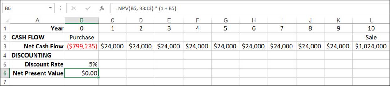
Figure 20.7 The net present value calculated using the NPV() function plus an adjustment.
Caution
Make sure that you adjust the discount rate to reflect the frequency of the discounting periods. If the periods are annual, the discount rate must be an annual rate. If the periods are monthly, you need to divide the discount rate by 12 to get the monthly rate.
Net Present Value with Varying Cash Flows
The major advantage of using NPV() over PV() is that NPV() can easily accommodate varying cash flows. You can use PV() directly to calculate the break-even purchase price, assuming that the asset or investment generates a constant cash flow each period. Alternatively, you can usePV() to help calculate the net present value for different cash flows if you build a complicated discounted cash flow model such as the one shown for the rental property in Figure 20.6.
You don’t need to worry about either of these scenarios if you use NPV(). That’s because you can simply enter the cash flows as the NPV() function’s values argument.
For example, suppose that you’re thinking of investing in a new piece of equipment that will generate income, but you don’t want to make the investment unless the machine will generate a return of at least 10% in today’s dollars over the first five years. Your cash-flow projection looks like this:
Year 0: $50,000 (purchase price)
Year 1: −$5,000
Year 2: $15,000
Year 3: $20,000
Year 4: $21,000
Year 5: $22,000
Figure 20.8 shows a worksheet that models this scenario with the cash flows in B4:G4. Using the target return of 10% as the discount rate (B6), the NPV() function returns $881 (B7). This amount is positive, which means that the machine will make at least a 10% return in today’s dollars over the first five years.
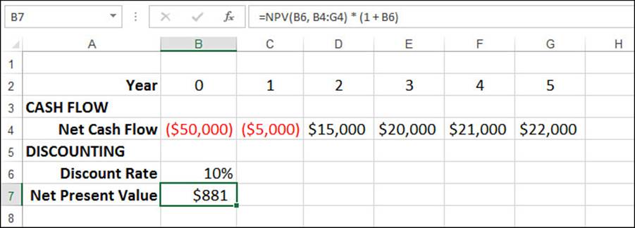
Figure 20.8 To see whether a series of cash flows meets a desired rate of return, use that rate as the discount rate in the NPV() function.
Net Present Value with Nonperiodic Cash Flows
The examples you’ve seen so far have assumed that the cash flows were periodic, meaning that they occur with the same frequency throughout the term (such as yearly or monthly). In some investments, however, the cash flows occur sporadically. In such a case, you can’t use the NPV()function, which works only with periodic cash flows.
Happily, Excel offers the XNPV() function, which can handle nonperiodic cash flows:
XNPV(rate, values, dates)
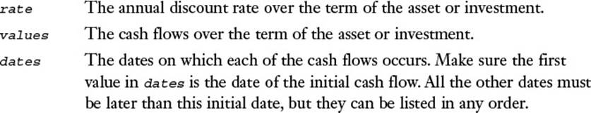
For example, Figure 20.9 shows a worksheet with a series of cash flows (B4:G4) and the dates on which they occur (B5:G5). Assuming a 10% discount rate (B7), the XNPV() function returns a value of $845, using the following formula (B8):
=XNPV(B7, B4:G5, B5:G5)
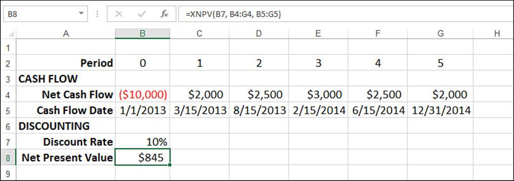
Figure 20.9 Use the XNPV() function to calculate the net present value for a series of nonperiodic cash flows.
Note
Note that the XNPV() function doesn’t have the missing-first-period quirk of the NPV() function. Therefore, you can use XNPV() straight up without adding a first-period factor.
Calculating the Payback Period
If you purchase a store, a piece of equipment, or an investment, your hope always is to at least recoup your initial outlay through the positive cash flows generated by the asset. The point at which you recoup the initial outlay is called the payback period. When analyzing a business case, one of the most common concerns is when the payback period occurs: A short payback period is better than a long one.
Simple Undiscounted Payback Period
Finding the undiscounted payback period is a matter of calculating the cumulative cash flows and watching when they turn from negative to positive. The period that shows the first positive cumulative cash flow is the payback period.
For example, suppose you purchase a store for $500,000 and project the following cash flows:
As you can see, the cumulative cash flow turns positive in year 6, so that’s the payback period.
Instead of simply eyeballing the payback period, you can use a formula to calculate it. Figure 20.10 shows a worksheet that lists the cash flows and uses the following array formula to calculate the payback period (see cell B5):
{=SUM(IF(SIGN(C4:I4) <> SIGN(OFFSET(C4:I4, 0, -1)), C1:I1, 0))}
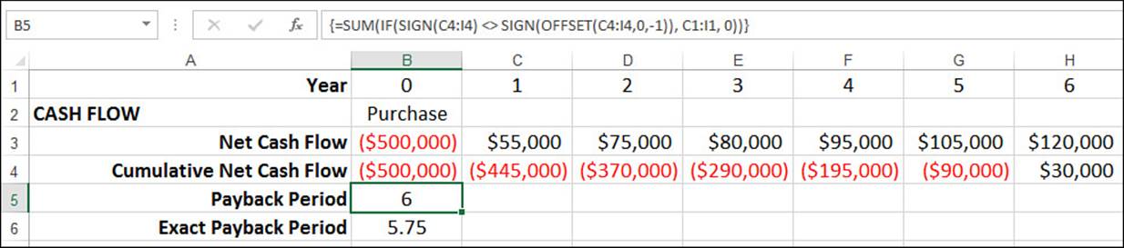
Figure 20.10 Use a formula to calculate the payback period.
The payback period occurs when the sign of the cumulative cash flows turns from negative to positive. Therefore, this formula uses IF() to compare each cumulative cash flow (C4:I4; you can ignore the first cash flow for this) with the cumulative cash flow from the previous period, as given by OFFSET(C4:I4, 0, -1). IF() returns 0 for all cases in which the signs are the same, and it returns the year value from row 1 (C1:I1) for the case in which the sign changes. Summing these values returns the year in which the sign changed, which is the payback period.
Exact Undiscounted Payback Point
If the income generated by the asset is always received at the end of the period, your analysis of the payback period is done. However, many assets generate income throughout the period. In this case, the payback period tells you that sometime within the period, the cumulative cash flows reaches 0. It might be useful to calculate exactly when during the period the payback occurs. Assuming that the income is received at regular intervals throughout the period, you can find the exact payback point by comparing how much is required to reach the payback with how much was earned during the payback period.
For example, suppose that the cumulative cash flow value was −$50,000 at the end of the previous period and that the asset generates $100,000 during the payback period. Assuming regular cash flow throughout the period, this means that the first $50,000 brought the cumulative cash flow to0. Because this is half the amount earned in the payback period, you can say that the exact payback point occurred halfway through the period.
More generally, you can use the following formula to calculate the exact payback point:
=Payback Period - Cumulative Cash Flow at Payback / Cash Flow at Payback
For example, suppose you know that the store’s payback period occurs in year 6, that the cumulative cash flow after year 6 is $30,000, and that the cash flow for year 6 was $120,000. Here’s the formula:
=6 - 30,000 / 120,000
The answer is 5.75, meaning that the exact payback point occurs three-quarters of the way through the sixth year.
To derive this in a worksheet, you first calculate the payback period and then use this number in the INDEX() function to return the values for the payback period’s cumulative cash flow and net cash flow. Here’s the formula used in Figure 20.11:
=B5 - INDEX(B4:H4, B5 + 1) / INDEX(B3:H3, B5 + 1)
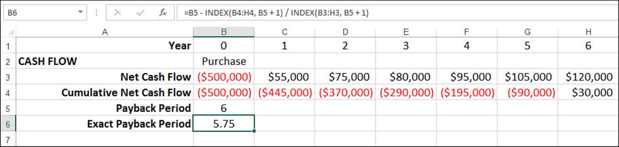
Figure 20.11 Use a formula to calculate the exact payback point.
Discounted Payback Period
Of course, the undiscounted payback period tells you only so much. To get a true measure of the payback, you need to apply these payback methods to the discounted cash flows. This tells you when the investment is paid back in today’s dollars.
To do this, you need to set up a schedule of discounted net cash flow and cumulative cash flow for each period and extend the periods until the cumulative discounted cash flow becomes positive. You can then use the formulas presented in the previous two sections (adjusted for the extra periods) to calculate the payback period and exact payback point (if applicable). Figure 20.12 shows the discounted payback values for the store’s cash flows.
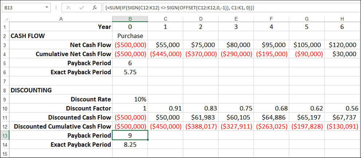
Figure 20.12 To derive the discounted payback values, create a schedule of discounted cash flows, extend the periods until the cumulative discounted cash flow turns positive, and then apply the payback formulas.
Calculating the Internal Rate of Return
In the earlier example with varying cash flows, the discount rate was set to 10% because that was the minimum return required in today’s dollars over the first five years after purchasing the equipment. This rate of return of an investment based on today’s dollars is called the internal rate of return. It’s actually defined as the discount rate required to get a net present value of $0.
In the equipment example, using a discount rate of 10% produced a net present value of $881. This is a positive amount, which means that the equipment actually produced an internal rate of return higher than 10%. What, then, was the actual internal rate of return?
Using the IRR() Function
You could figure this out by adjusting the discount rate up (in this case) until the NPV() calculation returns 0. However, Excel offers an easier method in the form of the IRR() function:
IRR(values[, guess])

Caution
The IRR() function’s values argument must contain at least one positive value and one negative value. If all the values have the same sign, the function returns the #NUM! error.
Figure 20.13 shows the cash flows generated by the equipment purchase and the resulting internal rate of return (cell B7) calculated by the IRR() function:
=IRR(B3:G3)
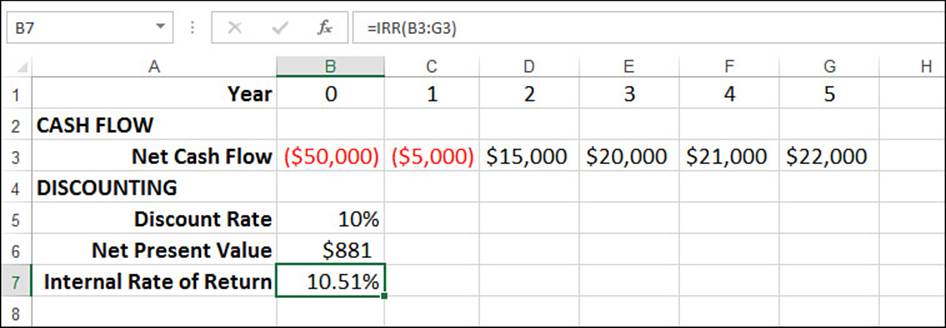
Figure 20.13 Use the IRR() function to calculate the internal rate of return for a series of periodic cash flows.
The calculated value of 10.51% means that plugging this value into the NPV() function as the discount rate would return a net present value of 0.
Note
The IRR() function uses iteration to find a solution that is accurate to within 0.00001%. If it can’t find a solution within 20 iterations, it returns the #NUM! error. If this happens, try using a different value for the guess argument.
Calculating the Internal Rate of Return for Nonperiodic Cash Flows
As with NPV(), the IRR() function works only with periodic cash flows. If your cash flows are nonperiodic, use the XIRR() function instead:
XIRR(values, dates[, guess])
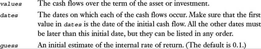
Figure 20.14 shows a worksheet with nonperiodic cash flows and the resulting internal rate of return (cell B8) calculated using the XIRR() function:
=XIRR(B3:G3, B4:G4)
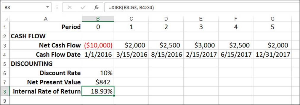
Figure 20.14 Use the XIRR() function to calculate the internal rate of return for a series of nonperiodic cash flows.
Calculating Multiple Internal Rates of Return
Rarely does a business pay cash for major capital investments. Instead, some or all of the purchase price is usually borrowed from the bank. When calculating the internal rate of return, two assumptions are made:
![]() The discount for negative cash flows is money paid to the bank to service borrowed money.
The discount for negative cash flows is money paid to the bank to service borrowed money.
![]() The discount for positive cash flows is money reinvested.
The discount for positive cash flows is money reinvested.
However, a third assumption also is at work when you use the IRR() function: The finance rate for negative cash flows and the reinvestment rate for positive cash flows are the same. In the real world, this is rarely true: Most banks charge interest for a loan that is 2 to 4 points higher than what you can usually get for an investment.
To handle the difference between the finance rate and the reinvestment rate, Excel enables you to calculate the modified internal rate of return using the MIRR() function:
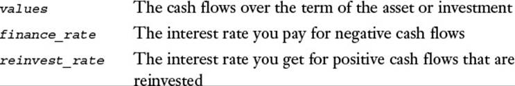
MIRR(values, finance_rate, reinvest_rate)
For example, suppose you’re charged 8% for loans, and you can get 6% for investments. Figure 20.15 shows a worksheet that calculates the modified internal rate of return based on the cash flows in B3:G3 and these rates:
=MIRR(B3:G3, B5, B6)
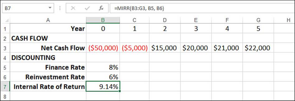
Figure 20.15 Use the MIRR() function to calculate the modified internal rate of return when you’re charged one rate for negative cash flows and a different rate for positive cash flows.
Case Study: Publishing a Book
Let’s put some of this cash-flow analysis to work in an example that, although still simplified, is more realistically detailed than the ones you’ve seen so far in this chapter. Specifically, this case study looks at the business case of publishing a book, taking into account the costs involved (both up front and ongoing) and the positive cash flow generated by the book. The cash-flow analysis will calculate the book’s payback period (undiscounted and discounted), as well as the yearly values for the net present value and the internal rate of return.
Per-Unit Constants
In publishing, many of the calculations involving both operating costs and sales are performed using per-unit (that is, per-book) constants. This case study uses the following six constants, as shown in Figure 20.16:
![]() List Price—The suggested retail price of the book
List Price—The suggested retail price of the book
![]() Average Customer Discount—The amount taken off the retail price when selling the book to bookstores
Average Customer Discount—The amount taken off the retail price when selling the book to bookstores
![]() PP&B—The per-unit costs for paper, printing, and binding
PP&B—The per-unit costs for paper, printing, and binding
![]() Cost of Sales—The per-unit costs of selling the book, including commissions, distribution, and so on
Cost of Sales—The per-unit costs of selling the book, including commissions, distribution, and so on
![]() Author Royalty—The percentage of the list price that the author receives
Author Royalty—The percentage of the list price that the author receives
![]() Margin—The per-unit margin, which is the list price minus the customer discount, PP&B, cost of sales, and author royalty, divided by the list price
Margin—The per-unit margin, which is the list price minus the customer discount, PP&B, cost of sales, and author royalty, divided by the list price
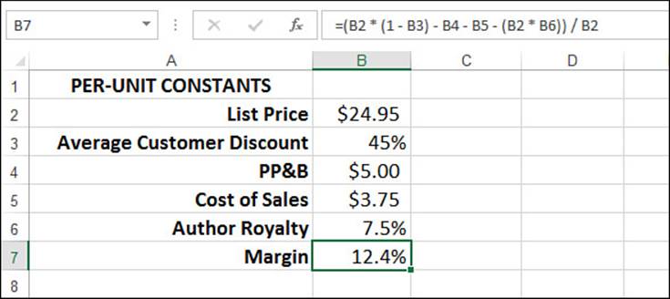
Figure 20.16 The per-unit constants used in the operating cost and sales calculations.
Operating Costs and Sales
Figure 20.17 shows the annual operating costs and sales for the book over 10 years. For the references to cells B2 through B7 in the following list of costs and sales, see Figure 20.16:
![]() Units Printed—The number of books printed during the year.
Units Printed—The number of books printed during the year.
![]() Units Sold—The number of units sold during the year.
Units Sold—The number of units sold during the year.
![]() New Title Costs—Costs associated with producing the book, including acquiring, editing, indexing, and so on.
New Title Costs—Costs associated with producing the book, including acquiring, editing, indexing, and so on.
![]() Total PP&B—The total paper, printing, and binding costs during the year. This is the year’s Units Printed value (from row 10) multiplied by the PP&B value (B4).
Total PP&B—The total paper, printing, and binding costs during the year. This is the year’s Units Printed value (from row 10) multiplied by the PP&B value (B4).
![]() Marketing—The marketing and publicity costs during the year.
Marketing—The marketing and publicity costs during the year.
![]() Total Cost of Sales—The total cost of sales during the year. This is the year’s Units Sold value (from row 11) multiplied by the Cost of Sales value (B5).
Total Cost of Sales—The total cost of sales during the year. This is the year’s Units Sold value (from row 11) multiplied by the Cost of Sales value (B5).
![]() Author Advance—The advance on royalties paid to the author. The assumption is that this value is paid at the beginning of the project, so it’s placed in year 0.
Author Advance—The advance on royalties paid to the author. The assumption is that this value is paid at the beginning of the project, so it’s placed in year 0.
![]() Author Royalties—The royalties paid to the author during the year. This is generally the year’s Units Sold value (from row 11) multiplied by the List Price (B2) and the Author Royalty (B6). However, the formula also takes into account the Author Advance, and it doesn’t pay royalties until the advance has earned out.
Author Royalties—The royalties paid to the author during the year. This is generally the year’s Units Sold value (from row 11) multiplied by the List Price (B2) and the Author Royalty (B6). However, the formula also takes into account the Author Advance, and it doesn’t pay royalties until the advance has earned out.
![]() $ Sales—The total sales, in dollars, during the year. This is the year’s Unit Sold value (from row 11) multiplied by the List Price (B2) minus the Average Customer Discount (B3).
$ Sales—The total sales, in dollars, during the year. This is the year’s Unit Sold value (from row 11) multiplied by the List Price (B2) minus the Average Customer Discount (B3).
![]() Translation Rights—Payments for translation rights sold during the year.
Translation Rights—Payments for translation rights sold during the year.
![]() Book Club Rights—Payments for book club rights sold during the year.
Book Club Rights—Payments for book club rights sold during the year.
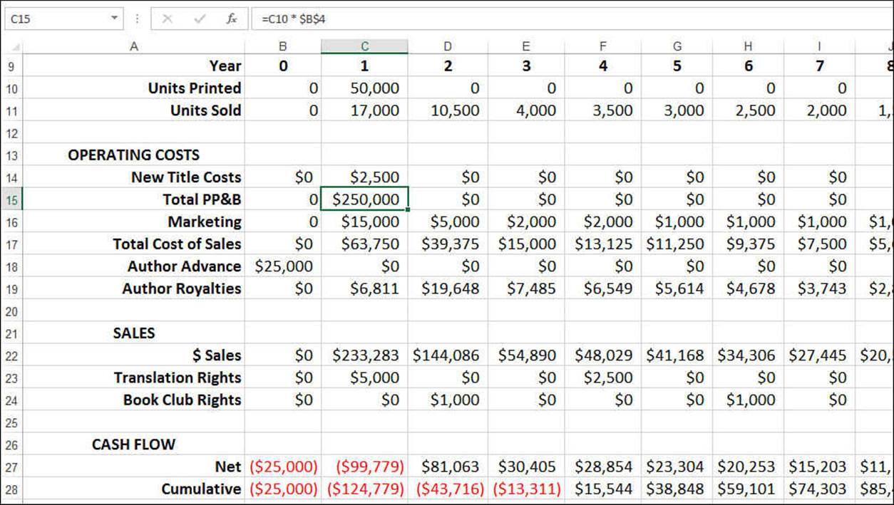
Figure 20.17 The operating costs and sales for each year.
Cash Flow
With the operating costs and sales available, you can calculate the net cash flow for each year by subtracting the sum of the operating costs from the sum of the sales. Figure 20.18 shows the book’s net cash flows in row 27, as well as its cumulative net cash flows (row 28). You also get the discounted net and cumulative cash flows using a discount rate of 12.4%. This is the same as the per-unit Margin value (B7 from Figure 20.16), and it is the target rate of return for the book.
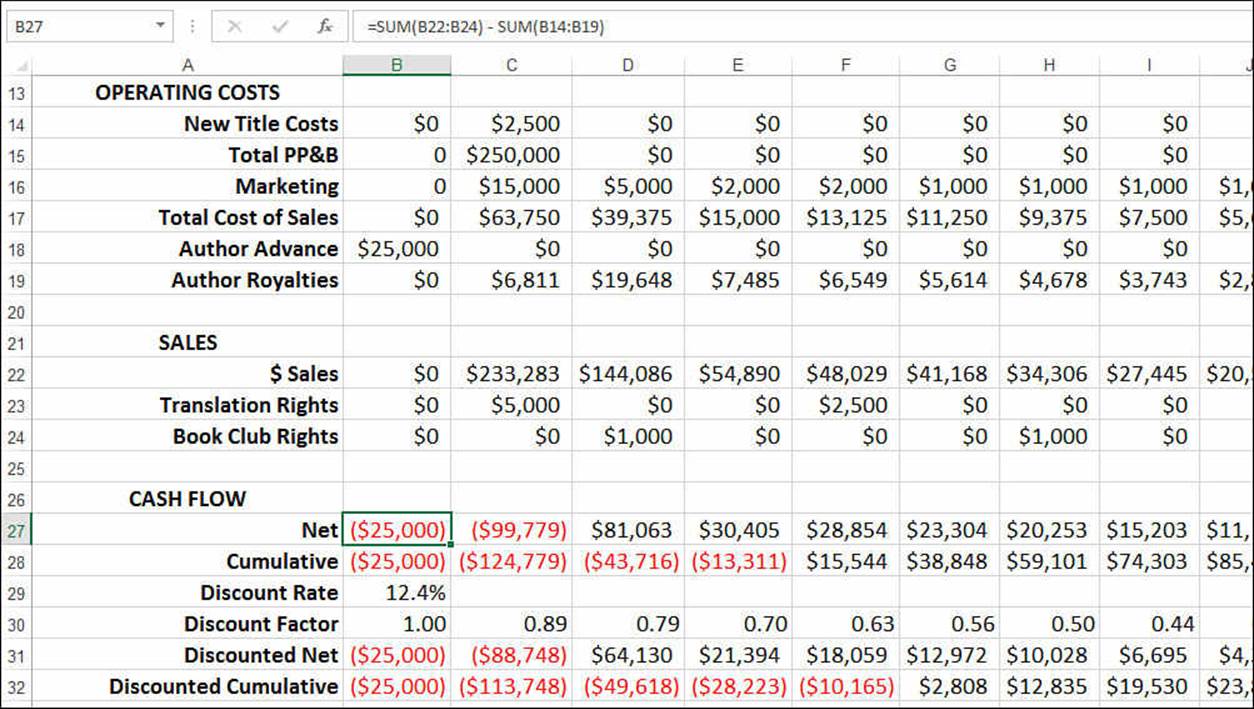
Figure 20.18 The yearly net and cumulative cash flows and their discounted versions.
Cash-Flow Analysis
Finally, you’re ready to analyze the cash flow, as shown in Figure 20.19. There are six values:
![]() Undiscounted Payback Period—The year in which the book’s undiscounted cumulative cash flows turn positive.
Undiscounted Payback Period—The year in which the book’s undiscounted cumulative cash flows turn positive.
![]() Undiscounted Payback Point—The exact point in the payback period at which the book’s undiscounted cumulative cash flows turn positive.
Undiscounted Payback Point—The exact point in the payback period at which the book’s undiscounted cumulative cash flows turn positive.
![]() Discounted Payback Period—The year in which the book’s discounted cumulative cash flows turn positive.
Discounted Payback Period—The year in which the book’s discounted cumulative cash flows turn positive.
![]() Discounted Payback Point—The exact point in the payback period at which the book’s discounted cumulative cash flows turn positive.
Discounted Payback Point—The exact point in the payback period at which the book’s discounted cumulative cash flows turn positive.
![]() Net Present Value—The net present value calculation at the end of each year, as returned by the NPV() function (with the fudge factor added, as explained earlier; see “Calculating Net Present Value Using NPV()”).
Net Present Value—The net present value calculation at the end of each year, as returned by the NPV() function (with the fudge factor added, as explained earlier; see “Calculating Net Present Value Using NPV()”).
![]() Internal Rate of Return—The internal rate of return calculation at the end of each year, as returned by the IRR() function. Note that we don’t start this calculation until year 2 because in year 1 there are nothing but negative cash flows.
Internal Rate of Return—The internal rate of return calculation at the end of each year, as returned by the IRR() function. Note that we don’t start this calculation until year 2 because in year 1 there are nothing but negative cash flows.
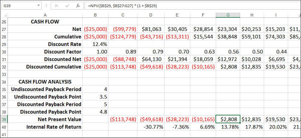
Figure 20.19 The cash-flow analysis for the book example.
Note
To get the internal rate of return for year 2 (cell D40), I had to use -0.1 as the guess argument for the IRR() function:
=IRR($B$27:D27, -0.1)
Without this initial estimate, Excel can’t complete the iteration, and it returns the #NUM! error.
From Here
![]() The IRR() and MIRR() functions use iteration to calculate results. To learn more about iteration, see “Using Iteration and Circular References,” p. 93.
The IRR() and MIRR() functions use iteration to calculate results. To learn more about iteration, see “Using Iteration and Circular References,” p. 93.
![]() To get the details on the time value of money, see “Understanding the Time Value of Money,” p. 433.
To get the details on the time value of money, see “Understanding the Time Value of Money,” p. 433.
![]() To use the PV() function in a loan context, see “Calculating How Much You Can Borrow,” p. 446.
To use the PV() function in a loan context, see “Calculating How Much You Can Borrow,” p. 446.
![]() To use the PV() function in an investment context, see “Calculating the Required Initial Deposit,” p. 461.
To use the PV() function in an investment context, see “Calculating the Required Initial Deposit,” p. 461.
![]() For the details on compound interest, see “Understanding Compound Interest,” p. 454.
For the details on compound interest, see “Understanding Compound Interest,” p. 454.
All materials on the site are licensed Creative Commons Attribution-Sharealike 3.0 Unported CC BY-SA 3.0 & GNU Free Documentation License (GFDL)
If you are the copyright holder of any material contained on our site and intend to remove it, please contact our site administrator for approval.
© 2016-2026 All site design rights belong to S.Y.A.