Excel® 2016 Formulas and Functions (2016)
Part I: Mastering Excel Ranges and Formulas
3. Building Basic Formulas
In This Chapter
Understanding Formula Basics
Understanding Operator Precedence
Controlling Worksheet Calculation
Copying and Moving Formulas
Displaying Worksheet Formulas
Converting a Formula to a Value
Working with Range Names in Formulas
Working with Links in Formulas
Formatting Numbers, Dates, and Times
A worksheet is merely a lifeless collection of numbers and text until you define some kind of relationship among the various entries. You do this by creating formulas that perform calculations and produce results. This chapter takes you through some formula basics, including constructing simple arithmetic and text formulas, understanding the all-important topic of operator precedence, copying and moving worksheet formulas, and making formulas easier to build and read by taking advantage of range names.
Understanding Formula Basics
Most worksheets are created to provide answers to specific questions: What is the company’s profit? Are expenses over or under budget, and by how much? What is the future value of an investment? How big will an employee’s bonus be this year? You can answer these questions, and an infinite number of others, by using Excel formulas.
All Excel formulas have the same general structure: an equal sign (=) followed by one or more operands, which can be values, cell references, ranges, range names, or function names, separated by one or more operators, which are symbols that combine the operands in some way, such as the plus sign (+) and the greater-than sign (>).
Note
Excel doesn’t object if you use spaces between operators and operands in your formulas. This is actually a good practice to get into because separating the elements of a formula in this way can make them much easier to read. Note, too, that Excel accepts line breaks in formulas. This is handy if you have a very long formula because it enables you to “break up” the formula so that it appears on multiple lines. To create a line break within a formula, press Alt+Enter.
Formula Limits in Excel 2016
It’s a good idea to know the limits Excel sets on various aspects of formulas and worksheet models, even though it’s unlikely that you’ll ever bump up against these limits. Formula limits that were expanded in Excel 2007 remain the same in Excel 2016. So, in the unlikely event that you’re coming to Excel 2016 from Excel 2003 or earlier, Table 3.1 shows you the updated limits.
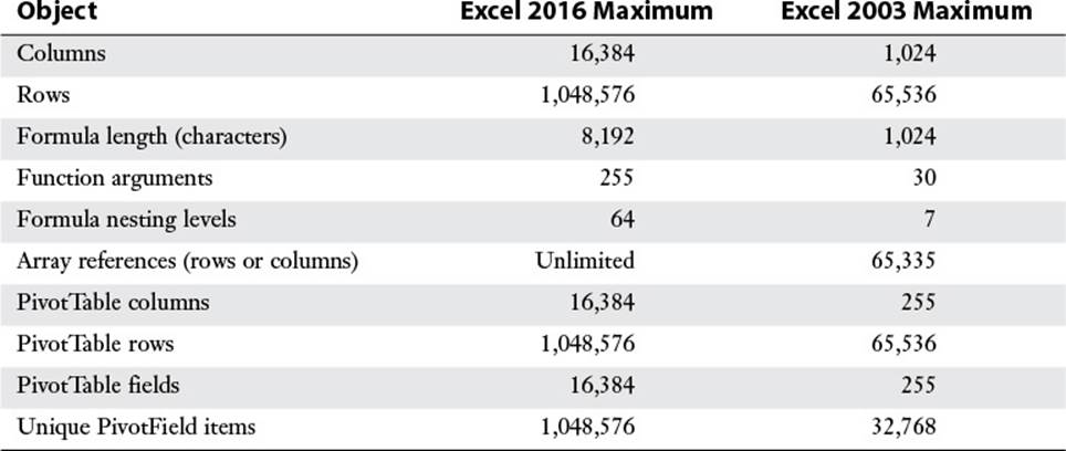
Table 3.1 Formula-Related Limits in Excel 2016
![]() Formula nesting levels refers to the number of expressions that are nested within other expressions using parentheses; see “Controlling the Order of Precedence,” p. 58.
Formula nesting levels refers to the number of expressions that are nested within other expressions using parentheses; see “Controlling the Order of Precedence,” p. 58.
Entering and Editing Formulas
Entering a new formula into a worksheet appears to be a straightforward process:
1. Select the cell in which you want to enter the formula.
2. Type an equal sign (=) to tell Excel that you’re entering a formula.
3. Type the formula’s operands and operators.
4. Press Enter to confirm the formula.
However, Excel has three different input modes that determine how it interprets certain keystrokes and mouse actions:
![]() When you type the equal sign to begin the formula, Excel goes into Enter mode, which is the mode you use to enter text (such as the formula’s operands and operators).
When you type the equal sign to begin the formula, Excel goes into Enter mode, which is the mode you use to enter text (such as the formula’s operands and operators).
![]() If you press any keyboard navigation key (such as Page Up, Page Down, or any arrow key), or if you click any other cell in the worksheet, Excel enters Point mode. This is the mode you use to select a cell or range as a formula operand. When you’re in Point mode, you can use any of the standard range-selection techniques. Note that Excel returns to Enter mode as soon as you type an operator or any character.
If you press any keyboard navigation key (such as Page Up, Page Down, or any arrow key), or if you click any other cell in the worksheet, Excel enters Point mode. This is the mode you use to select a cell or range as a formula operand. When you’re in Point mode, you can use any of the standard range-selection techniques. Note that Excel returns to Enter mode as soon as you type an operator or any character.
![]() If you press F2, Excel enters Edit mode, which is the mode you use to make changes to the formula. For example, when you’re in Edit mode, you can use the left and right arrow keys to move the cursor to another part of the formula for deleting or inserting characters. You can also enter Edit mode by clicking anywhere within the formula. Press F2 to return to Enter mode.
If you press F2, Excel enters Edit mode, which is the mode you use to make changes to the formula. For example, when you’re in Edit mode, you can use the left and right arrow keys to move the cursor to another part of the formula for deleting or inserting characters. You can also enter Edit mode by clicking anywhere within the formula. Press F2 to return to Enter mode.
Tip
You can tell which mode Excel is currently in by looking at the status bar. On the left side, you’ll see “Enter,” “Point,” or “Edit.”
After you’ve entered a formula, you might need to return to it to make changes. Excel gives you three ways to enter Edit mode and make changes to a formula in the selected cell:
![]() Press F2.
Press F2.
![]() Double-click the cell.
Double-click the cell.
![]() Use the formula bar to click anywhere inside the formula text.
Use the formula bar to click anywhere inside the formula text.
Excel divides formulas into four groups: arithmetic, comparison, text, and reference. Each group has its own set of operators, and you use each group in different ways. In the next few sections, I show you how to use each type of formula.
Using Arithmetic Formulas
Arithmetic formulas are by far the most common type of formula. They combine numbers, cell addresses, and function results with mathematical operators to perform calculations. Table 3.2 summarizes the mathematical operators used in arithmetic formulas.
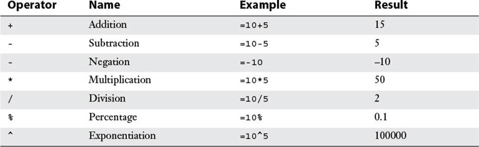
Table 3.2 The Arithmetic Operators
Most of these operators are straightforward, but the exponentiation operator might require further explanation. The formula =x^y means that the value x is raised to the power y. For example, the formula =3^2 produces the result 9 (that is, 3*3=9). Similarly, the formula =2^4 produces 16 (that is, 2*2*2*2=16).
Using Comparison Formulas
A comparison formula is a statement that compares two or more numbers, text strings, cell contents, or function results. If the statement is true, the result of the formula is given the logical value TRUE (which is equivalent to any nonzero value). If the statement is false, the formula returns the logical value FALSE (which is equivalent to zero). Table 3.3 summarizes the operators you can use in comparison formulas.
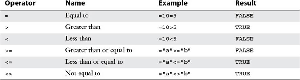
Table 3.3 Comparison Formula Operators
Comparison formulas have many uses. For example, you can determine whether to pay a salesperson a bonus by using a comparison formula to compare actual sales with a predetermined quota. If the sales are greater than the quota, the rep is awarded the bonus. You also can monitor credit collection. For example, if the amount a customer owes is more than 150 days past due, you might send the invoice to a collection agency.
![]() Comparison formulas also make use of Excel’s logical functions, so see “Adding Intelligence with Logical Functions,” p. 163.
Comparison formulas also make use of Excel’s logical functions, so see “Adding Intelligence with Logical Functions,” p. 163.
Using Text Formulas
The two types of formulas that I discussed in the previous sections, arithmetic formulas and comparison formulas, calculate or make comparisons and return values. A text formula, on the other hand, is a formula that returns text. Text formulas use the ampersand (&) operator to work with text cells, text strings enclosed in quotation marks, and text function results.
One way to use text formulas is to concatenate text strings. For example, if you enter the formula ="soft"&"ware" into a cell, Excel displays software. Note that the quotation marks and the ampersand aren’t shown in the result. You also can use & to combine cells that contain text. For example, if A1 contains the text Ben and A2 contains Jerry, entering the formula =A1&" and "&A2 returns Ben and Jerry.
![]() For other uses of text formulas, see Chapter 7, “Working with Text Functions,” p. 139.
For other uses of text formulas, see Chapter 7, “Working with Text Functions,” p. 139.
Using Reference Formulas
The reference operators combine two cell references or ranges to create a single joint reference. Table 3.4 summarizes the operators you can use in reference formulas.
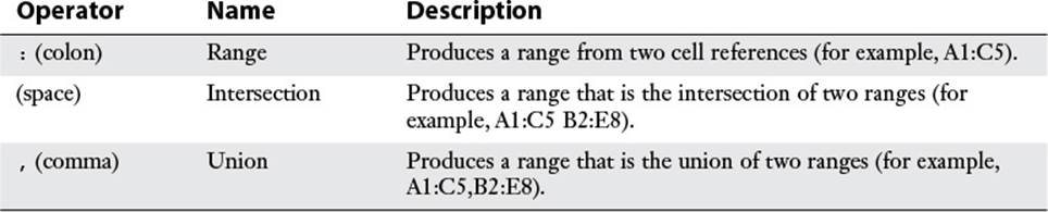
Table 3.4 Reference Formula Operators
Understanding Operator Precedence
You’ll often use simple formulas that contain just two values and a single operator. In practice, however, most formulas you use will have a number of values and operators. In more complex expressions, the order in which the calculations are performed becomes crucial. For example, consider the formula =3+5^2. If you calculate from left to right, the answer you get is 64 (3+5 equals 8, and 8^2 equals 64). However, if you perform the exponentiation first and then the addition, the result is 28 (5^2 equals 25, and 3+25 equals 28). As this example shows, a single formula can produce multiple answers, depending on the order in which you perform the calculations.
To control this problem, Excel evaluates a formula according to a predefined order of precedence. This order of precedence enables Excel to calculate a formula unambiguously by determining which part of the formula it calculates first, which part second, and so on.
The Order of Precedence
Excel’s order of precedence is determined by the various formula operators outlined earlier. Table 3.5 summarizes the complete order of precedence used by Excel.
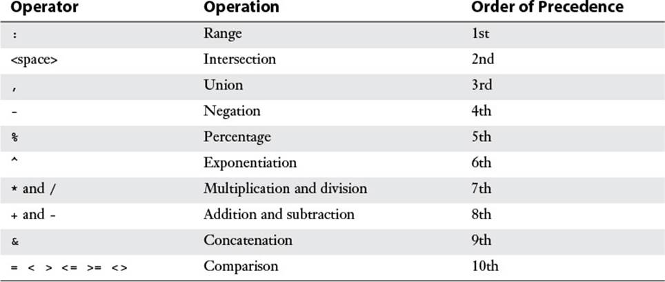
Table 3.5 The Excel Order of Precedence
From this table, you can see that Excel performs exponentiation before addition. Therefore, the correct answer for the formula =3+5^2, given previously, is 28. Notice also that some operators in Table 3.5 have the same order of precedence (for example, multiplication and division). This means that it usually doesn’t matter in which order these operators are evaluated. For example, consider the formula =5*10/2. If you perform the multiplication first, the answer you get is 25 (5*10 equals 50, and 50/2 equals 25). If you perform the division first, you also get an answer of 25 (10/2 equals 5, and 5*5 equals 25). By convention, Excel evaluates operators with the same order of precedence from left to right, so you should assume that’s how your formulas will be evaluated.
Controlling the Order of Precedence
Sometimes you want to override the order of precedence. For example, suppose that you want to create a formula that calculates the pre-tax cost of an item. If you bought something for $10.65, including 7% sales tax, and you want to find the cost of the item minus the tax, you use the formula =10.65/1.07, which gives you the correct answer, $9.95. In general, the formula is the total cost divided by 1 plus the tax rate, as shown in Figure 3.1.

Figure 3.1 The general formula to calculate the pre-tax cost of an item.
Figure 3.2 shows how you might implement such a formula. Cell B5 displays the Total Cost variable, and cell B6 displays the Tax Rate variable. Given these parameters, your first instinct might be to use the formula =B5/1+B6 to calculate the original cost. This formula is shown (as text) in cell E9, and the result is given in cell D9. As you can see, this answer is incorrect. What happened? Well, according to the rules of precedence, Excel performs division before addition, so the value in B5 first is divided by 1 and then is added to the value in B6. To get the correct answer, you must override the order of precedence so that the addition 1+B6 is performed first. You do this by surrounding that part of the formula with parentheses, as shown in cell E10. When this is done, you get the correct answer (cell D10).
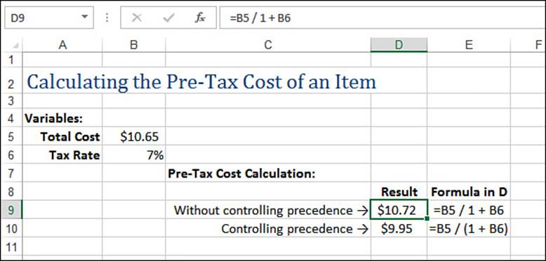
Figure 3.2 Use parentheses to control the order of precedence in your formulas.
Tip
In Figure 3.2, how did I convince Excel to show the formulas in cells E9 and E10 as text? I used Excel’s FORMULATEXT() function (see “Displaying a Cell’s Formula by Using FORMULATEXT(),” later in this chapter).
Note
You can download this chapter’s sample workbooks at www.mcfedries.com/books/book.php?title=excel-2016-formulas-and-functions.
In general, you can use parentheses to control the order that Excel uses to calculate formulas. Terms inside parentheses are always calculated first; terms outside parentheses are calculated sequentially (according to the order of precedence).
Tip
Another good use for parentheses is raising a number to a fractional power. For example, if you want to take the nth root of a number, you use the following general formula:
=number ^ (1 / n)
For example, to take the cube root of the value in cell A1, use this:
=A1 ^ (1 / 3)
To gain even more control over your formulas, you can place parentheses inside one another; this is called nesting parentheses. Excel always evaluates the innermost set of parentheses first. Here are a few sample formulas:
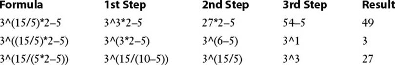
Notice that the order of precedence rules also hold within parentheses. For example, in the expression (5*2-5), the term 5*2 is calculated before 5 is subtracted.
Using parentheses to determine the order of calculations enables you to gain full control over your Excel formulas. This way, you can make sure that the answer given by a formula is the one you want.
Caution
One of the most common mistakes when using parentheses in formulas is to forget to close a parenthetic term with a right parenthesis. In such a case, Excel generates an error message (and offers a solution to the problem). To make sure that you’ve closed each parenthetic term, count all the left and right parentheses. If these totals don’t match, you know you’ve left out a parenthesis.
Controlling Worksheet Calculation
Excel always calculates a formula when you confirm its entry, and the program normally recalculates existing formulas automatically whenever their data changes. This behavior is fine for small worksheets, but it can slow you down if you have a complex model that takes several seconds or even several minutes to recalculate. To turn off this automatic recalculation, Excel gives you two ways to get started:
![]() Select Formulas, Calculation Options.
Select Formulas, Calculation Options.
![]() Select File, Options and then click Formulas.
Select File, Options and then click Formulas.
Either way, you’re presented with three calculation options:
![]() Automatic—This is the default calculation mode, and it means that Excel recalculates formulas as soon as you enter them and as soon as the data for a formula changes.
Automatic—This is the default calculation mode, and it means that Excel recalculates formulas as soon as you enter them and as soon as the data for a formula changes.
![]() Automatic Except for Data Tables—In this calculation mode, Excel recalculates all formulas automatically, except for those associated with data tables. This is a good choice if your worksheet includes one or more massive data tables that are slowing down the recalculation.
Automatic Except for Data Tables—In this calculation mode, Excel recalculates all formulas automatically, except for those associated with data tables. This is a good choice if your worksheet includes one or more massive data tables that are slowing down the recalculation.
![]() To learn how to set up data tables, see “Using What-If Analysis,” p. 349.
To learn how to set up data tables, see “Using What-If Analysis,” p. 349.
![]() Manual—Select this mode to force Excel not to recalculate any formulas until either you manually recalculate or you save the workbook. If you’re in the Excel Options dialog box, you can tell Excel not to recalculate when you save the workbook by clearing the Recalculate Workbook Before Saving check box.
Manual—Select this mode to force Excel not to recalculate any formulas until either you manually recalculate or you save the workbook. If you’re in the Excel Options dialog box, you can tell Excel not to recalculate when you save the workbook by clearing the Recalculate Workbook Before Saving check box.
With manual calculation turned on, you see “Calculate” in the status bar whenever your worksheet data changes and your formula results need to be updated. When you want to recalculate, first display the Formulas tab. In the Calculation group, you have two choices:
![]() Click Calculate Now (or press F9) to recalculate every open worksheet.
Click Calculate Now (or press F9) to recalculate every open worksheet.
![]() Click Calculate Sheet (or press Shift+F9) to recalculate only the active worksheet.
Click Calculate Sheet (or press Shift+F9) to recalculate only the active worksheet.
Tip
If you want Excel to recalculate every formula—even those that are unchanged—in all open worksheets, press Ctrl+Alt+Shift+F9.
If you want to recalculate only part of your worksheet while manual calculation is turned on, you have two options:
![]() To recalculate a single formula, select the cell containing the formula, click in the formula bar, and then confirm the cell (by pressing Enter or clicking the Enter button).
To recalculate a single formula, select the cell containing the formula, click in the formula bar, and then confirm the cell (by pressing Enter or clicking the Enter button).
![]() To recalculate a range, select the range; select Home, Find & Select, Replace (or press Ctrl+H); and enter an equal sign (=) in both the Find What and Replace With boxes. Click Replace All. Excel “replaces” the equal sign in each formula with another equal sign. This doesn’t actually change any formula, but it forces Excel to recalculate each formula.
To recalculate a range, select the range; select Home, Find & Select, Replace (or press Ctrl+H); and enter an equal sign (=) in both the Find What and Replace With boxes. Click Replace All. Excel “replaces” the equal sign in each formula with another equal sign. This doesn’t actually change any formula, but it forces Excel to recalculate each formula.
Tip
Excel supports multithreaded calculation on computers with either multiple processors or processors with multiple cores. For each processor (or core), Excel sets up a thread (a separate process of execution). Excel can then use each available thread to process multiple calculations concurrently. For a worksheet with multiple, independent formulas, this can dramatically speed up calculations. To make sure multithreaded calculation is turned on, select File, Options, click Advanced, and then in the Formulas section ensure that the Enable Multi-Threaded Calculation check box is selected.
Copying and Moving Formulas
You copy and move ranges that contain formulas the same way you copy and move regular ranges, but the results aren’t always straightforward.
For example, Figure 3.3 shows a list of expense data for a company. The formula in cell C11 uses the SUM() function to total the January expenses (range C6:C10). The idea behind this worksheet is to calculate a new expense budget number for 2016 as a percentage increase of the actual 2015 total. Cell C3 displays the INCREASE variable (in this case, the increase being used is 3%). The formula that calculates the 2016 BUDGET number (cell C13 for the month of January) multiplies the 2015 TOTAL by the INCREASE (that is, =C11*C3).
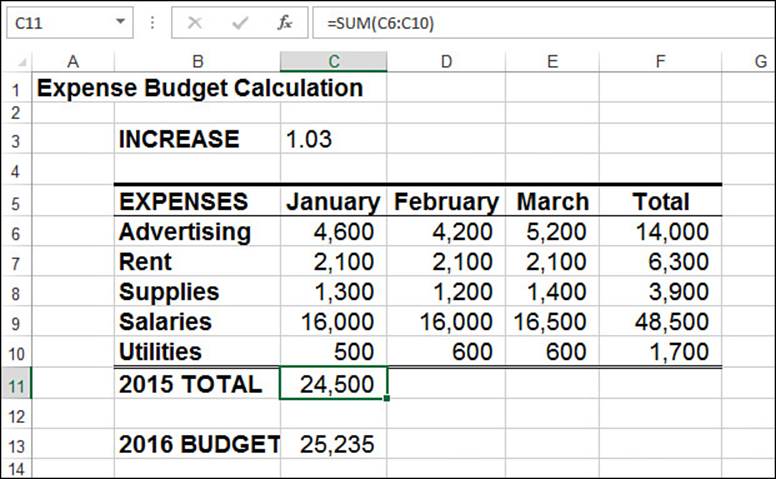
Figure 3.3 A budget expenses worksheet with two calculations for the January numbers: the total (cell C11) and a percentage increase for next year (cell C13).
The next step is to calculate the 2015 TOTAL expenses and the 2016 BUDGET figure for February. You could just type each new formula, but you can copy a cell much more quickly. Figure 3.4 shows the results when you copy the contents of cell C11 into cell D11. As you can see, Excel adjusts the range in the formula’s SUM() function so that only the February expenses (D6:D10) are totaled. How did Excel know to do this? To answer this question, you need to know about Excel’s relative reference format, which I discuss in the next section.
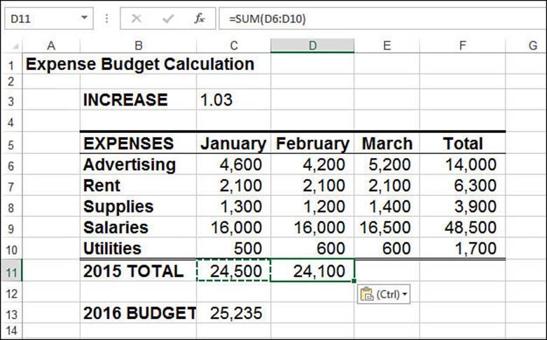
Figure 3.4 When you copy the January 2015 TOTAL formula to February, Excel automatically adjusts the range reference.
Understanding Relative Reference Format
When you use a cell reference in a formula, Excel looks at the cell address relative to the location of the formula. For example, suppose that you have the formula =A1*2 in cell A3. To Excel, this formula says, “Multiply the contents of the cell two rows above this one by 2.” This is called the relative reference format, and it’s the default format for Excel. This means that if you copy this formula to cell A4, the relative reference is still “Multiply the contents of the cell two rows above this one by 2,” but the formula changes to =A2*2 because A2 is two rows above A4.
Figure 3.4 shows why this format is useful. You had only to copy the formula in cell C11 to cell D11 and, thanks to relative referencing, everything came out perfectly. To get the expense total for March, you would just have to paste the same formula into cell E11. You’ll find that this way of handling copy operations will save you incredible amounts of time when you’re building worksheet models.
However, you need to exercise some care when copying or moving formulas. Let’s see what happens if you return to the budget expense worksheet and try copying the 2016 BUDGET formula in cell C13 to cell D13. Figure 3.5 shows that the result is 0!
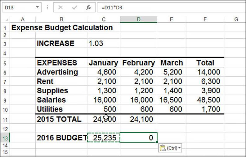
Figure 3.5 Copying the January 2016 BUDGET formula to February creates a problem.
What happened? The formula bar shows the problem: The new formula is =D11*D3. Cell D11 is the February 2015 TOTAL, and that’s fine, but instead of the INCREASE cell (C3), the formula refers to a blank cell (D3). Excel treats blank cells as 0, so the formula result is 0. The problem is the relative reference format. When the formula was copied, Excel assumed that the new formula should refer to cell D3. To see how you can correct this problem, you need to learn about another format, the absolute reference format, which I discuss in the next section.
Note
The relative reference format problem doesn’t occur when you move a formula. When you move a formula, Excel assumes that you want to keep the same cell references.
Understanding Absolute Reference Format
When you refer to a cell in a formula using the absolute reference format, Excel uses the physical address of the cell. You tell the program that you want to use an absolute reference by placing dollar signs ($) before the row and column of the cell address. To return to the example in the preceding section, Excel interprets the formula =$A$1*2 as “Multiply the contents of cell A1 by 2.” No matter where you copy or move this formula, the cell reference doesn’t change. The cell address is said to be anchored.
To fix the budget expense worksheet, you need to anchor the INCREASE variable. To do this, you first change the January 2016 BUDGET formula in cell C13 to read =C11*$C$3. After making this change, copying the formula to the February 2016 BUDGET column gives the new formula =D11*$C$3, which produces the correct result.
Caution
Most range names refer to absolute cell references. This means that when you copy a formula that uses a range name, the copied formula will use the same range name as the original. This might produce errors in your worksheet.
You also should know that you can enter a cell reference using a mixed-reference format. In this format, you anchor either the cell’s row (by placing the dollar sign in front of the row address only—for example, B$6) or its column (by placing the dollar sign in front of the column address only—for example, $B6).
Tip
You can quickly change the reference format of a cell address by using the F4 key. When editing a formula, place the cursor to the left of the cell address (or between the row and column values) and then keep pressing F4. Excel cycles through the various formats. When you see the format you want, press Enter. If you want to apply the new reference format to multiple cell addresses, highlight the addresses, press F4 until you get the format you want, and press Enter.
Copying a Formula Without Adjusting Relative References
If you need to copy a formula but don’t want the formula’s relative references to change, follow these steps:
1. Select the cell that contains the formula you want to copy.
2. Click inside the formula bar to activate it.
3. Use the mouse or keyboard to select the entire formula.
4. Copy the selected formula.
5. Press Esc to deactivate the formula bar.
6. Select the cell in which you want the copy of the formula to appear.
7. Paste the formula.
Note
Here are two other methods you can use to copy a formula without adjusting its relative cell references:
![]() To copy a formula from the cell above, select the lower cell and press Ctrl+’ (apostrophe).
To copy a formula from the cell above, select the lower cell and press Ctrl+’ (apostrophe).
![]() Activate the formula bar and type an apostrophe (’) at the beginning of the formula (that is, to the left of the equal sign) to convert it to text. Press Enter to confirm the edit, copy the cell, and then paste it in the desired location. Now, delete the apostrophe from both the source and destination cells to convert the text back to a formula.
Activate the formula bar and type an apostrophe (’) at the beginning of the formula (that is, to the left of the equal sign) to convert it to text. Press Enter to confirm the edit, copy the cell, and then paste it in the desired location. Now, delete the apostrophe from both the source and destination cells to convert the text back to a formula.
Displaying Worksheet Formulas
By default, Excel displays in a cell the results of the cell’s formula instead of the formula itself. If you need to see a formula, you can simply select the appropriate cell and look at the formula bar. However, sometimes you’ll want to see all the formulas in a worksheet (such as when you’re troubleshooting your work).
![]() For more information about solving formula problems, see Chapter 5, “Troubleshooting Formulas,” p. 111.
For more information about solving formula problems, see Chapter 5, “Troubleshooting Formulas,” p. 111.
Displaying All Worksheet Formulas
To display all of a worksheet’s formulas, select Formulas, Show Formulas.
Tip
You can also press Ctrl+` (backquote) to toggle a worksheet between values and formulas.
Displaying a Cell’s Formula by Using FORMULATEXT()
In some cases, rather than showing all of a sheet’s formulas, you might prefer to show the formulas in only a cell or two. For example, if you’re presenting a worksheet to other people, that sheet might have some formulas you want to show, but it might also have one or more proprietary formulas that you don’t want your audience to see. In such a case, you can display individual cell formulas by using the FORMULATEXT() function:
FORMULATEXT(cell)
![]()
For example, the following formula displays the formula text from cell D9:
=FORMULATEXT(D9)
Converting a Formula to a Value
If a cell contains a formula whose value will never change, you can convert the formula to that value. This speeds up large worksheet recalculations and frees up memory for your worksheet because values use much less memory than formulas do. For example, you might have formulas in part of your worksheet that use values from a previous fiscal year. Because these numbers aren’t likely to change, you can safely convert the formulas to their values. To do this, follow these steps:
1. Select the cell containing the formula you want to convert.
2. Double-click the cell or press F2 to activate in-cell editing.
3. Press F9. The formula changes to its value.
4. Press Enter or click the Enter button. Excel changes the cell to the value.
You’ll often need to use the result of a formula in several places. If a formula is in cell C5, for example, you can display its result in other cells by entering =C5 in each of the cells. This is the best method if you think the formula result might change because, if it does, Excel updates the other cells automatically. However, if you’re sure that the result won’t change, you can copy only the value of the formula into the other cells. Use the following procedure to do this:
1. Select the cell that contains the formula.
2. Copy the cell.
3. Select the cell or cells to which you want to copy the value.
4. Select Home, display the Paste list, and then select Paste Values. Excel pastes the cell’s value to each cell you selected.
Another method is to copy the cell, paste it into the destination, drop down the Paste Options list, and then select Values Only.
Caution
If your worksheet is set to manual calculation, make sure that you update your formulas (by pressing F9) before copying the values of your formulas.
Working with Range Names in Formulas
In Chapter 2, “Using Range Names,” you saw how to define and use range names in worksheets. You probably use range names often in your formulas. After all, a cell that contains the formula =Sales-Expenses is much more comprehensible than one that contains the more cryptic formula =F12-F3. The next few sections show you some techniques that make it easier to use range names in formulas.
Pasting a Name into a Formula
One way to enter a range name in a formula is to type the name in the formula bar. But what if you can’t remember the name? Or what if the name is long, and you’ve got a deadline looming? For these kinds of situations, Excel has several features that enable you to select the name you want from a list and paste it right into the formula. Start your formula, and when you get to the spot where you want the name to appear, use any of the following techniques:
![]() Select Formulas, Use in Formula and then click the name in the list that appears (see Figure 3.6).
Select Formulas, Use in Formula and then click the name in the list that appears (see Figure 3.6).
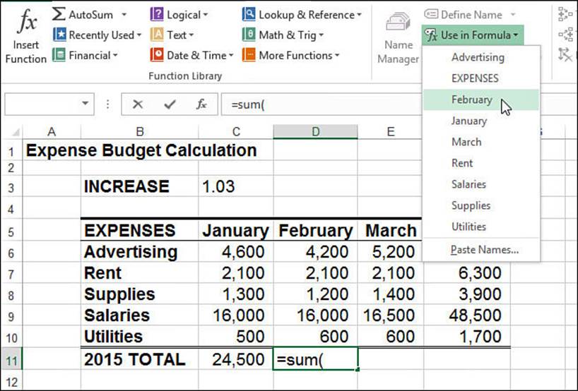
Figure 3.6 Drop down the Use in Formula list and then click the range name you want to insert into your formula.
![]() Select Formulas, Use in Formula, Paste Names (or press F3) to display the Paste Name dialog box, click the range name you want to use, and then click OK.
Select Formulas, Use in Formula, Paste Names (or press F3) to display the Paste Name dialog box, click the range name you want to use, and then click OK.
![]() Type the first letter or two of the range name to display a list of names and functions that start with those letters, select the name you want, and then press Tab.
Type the first letter or two of the range name to display a list of names and functions that start with those letters, select the name you want, and then press Tab.
Applying Names to Formulas
If you’ve been using ranges in your formulas and you name those ranges later, Excel doesn’t automatically apply the new names to the formulas. Instead of substituting the appropriate names by hand, you can get Excel to do the hard work for you. Follow these steps to apply the new range names to your existing formulas:
1. Select the range in which you want to apply the names or select a single cell if you want to apply the names to the entire worksheet.
2. Select Formulas, Define Name, Apply Names. Excel displays the Apply Names dialog box, shown in Figure 3.7.
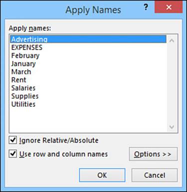
Figure 3.7 Use the Apply Names dialog box to select the names you want to apply to your formula ranges.
3. In the Apply Names list, choose the name or names you want applied from this list.
4. Select the Ignore Relative/Absolute check box to ignore relative and absolute references when applying names. (See the next section for more information on this option.)
5. Select the Use Row and Column Names check box to tell Excel whether to use the worksheet’s row and column names when applying names. If you select this check box, you also can click the Options button to see more choices. (See the section “Using Row and Column Names When Applying Names,” later in this chapter, for details.)
6. Click OK to apply the names.
Ignoring Relative and Absolute References When Applying Names
If you clear the Ignore Relative/Absolute option in the Apply Names dialog box, Excel replaces relative range references only with names that refer to relative references, and it replaces absolute range references only with names that refer to absolute references. If you leave this option selected, Excel ignores relative and absolute reference formats when applying names to a formula.
For example, suppose that you have a formula such as =SUM(A1:A10) and a range named Sales that refers to $A$1:$A$10. With the Ignore Relative/Absolute option turned off, Excel won’t apply the name Sales to the range in the formula; Sales refers to an absolute range, and the formula contains a relative range. Unless you think you’ll be moving your formulas around, you should leave the Ignore Relative/Absolute option selected.
Using Row and Column Names When Applying Names
For extra clarity in your formulas, leave the Use Row and Column Names check box selected in the Apply Names dialog box. This option tells Excel to rename all cell references that can be described as the intersection of a named row and a named column. In Figure 3.8, for example, the range C6:C10 is named January, and the range C7:E7 is named Rent. This means that cell C7—the intersection of these two ranges—can be referenced as January Rent.
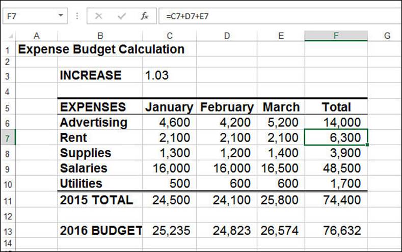
Figure 3.8 Before range names are applied to the formulas, cell F7 (Total Rent) contains the formula =C7+D7+E7.
As shown in Figure 3.8, the Total for the Rent row (cell F7) currently contains the formula =C7+D7+E7. If you applied range names to this worksheet and selected the Use Row and Column Names option, you’d think this formula would be changed to this:
=January Rent + February Rent + March Rent
If you try this, however, you’ll get a slightly different formula, as shown in Figure 3.9.
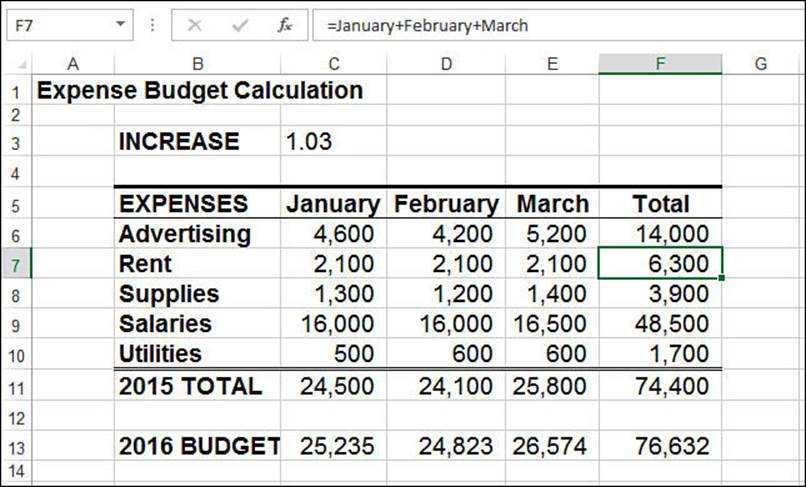
Figure 3.9 After range names are applied, the Total Rent cell contains the formula =January+February+March.
The reason for this is that when Excel is applying names, it omits the row name if the formula is in the same row. (It also omits the column name if the formula is in the same column.) In cell F7, for example, Excel omits Rent in each term because F7 is in the Rent row.
Omitting row headings isn’t a problem in a small model, but it can be confusing in a large worksheet, where you might not be able to see the names of the rows. Therefore, if you’re applying names to a large worksheet, you’ll probably prefer to include the row names when applying names.
Choosing the Options button in the Apply Names dialog box displays the expanded dialog box shown in Figure 3.10. This includes extra options that enable you to include column (and row) headings:
![]() Omit Column Name if Same Column—Clear this check box to include column names when applying names.
Omit Column Name if Same Column—Clear this check box to include column names when applying names.
![]() Omit Row Name if Same Row—Clear this check box to include row names.
Omit Row Name if Same Row—Clear this check box to include row names.
![]() Name Order—Use these options (Row Column or Column Row) to select the order of names in the reference.
Name Order—Use these options (Row Column or Column Row) to select the order of names in the reference.
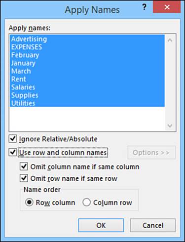
Figure 3.10 The expanded Apply Names dialog box.
Naming Formulas
In Chapter 2, you learned how to set up names for often-used constants. You can apply a similar naming concept for frequently used formulas. As with the constants, the formula doesn’t physically have to appear in a cell. This not only saves memory but often makes your worksheets easier to read as well. Follow these steps to name a formula:
1. Select Formulas, Define Name to display the New Name dialog box.
2. Enter the name you want to use for the formula in the Name text box.
3. In the Refers To box, enter the formula exactly as you would if you were entering it in a worksheet.
4. Click OK.
Now you can enter the formula name in your worksheet cells (instead of the formula itself). For example, the following is the formula for the volume of a sphere (r is the radius of the sphere):
4πr3/3
So, assuming that you have a cell named Radius somewhere in the workbook, you could create a formula named, say, SphereVolume, and make the following entry in the Refers To box of the New Name dialog box (where PI() is the Excel worksheet function that returns the value of pi):
=(4 * PI() * Radius ^ 3) / 3
Working with Links in Formulas
If you have data in one workbook that you want to use in another, you can set up a link between the two workbooks. This action enables your formulas to use references to cells or ranges in the other workbook. When the other data changes, Excel automatically updates the link.
For example, Figure 3.11 shows two linked workbooks. The Budget Summary sheet in the 2017 Budget-Summary workbook includes data from the Details worksheet in the 2017 Budget workbook. Specifically, the formula shown for cell B2 in 2017 Budget-Summary contains an external reference to cell R7 in the Details worksheet of 2017 Budget. If the value in R7 changes, Excel immediately updates the 2017 Budget-Summary workbook.
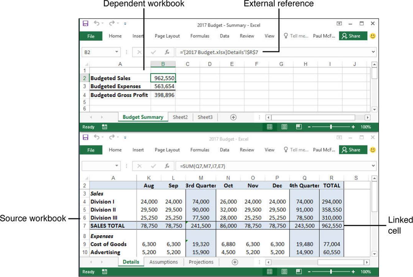
Figure 3.11 These two workbooks are linked because the formula in cell B2 of the 2017 Budget-Summary workbook references cell R7 in the 2017 Budget workbook.
Note
The workbook that contains the external reference is called the dependent workbook (or the client workbook). The workbook that contains the original data is called the source workbook (or the server workbook).
Understanding External References
There’s no big mystery behind external reference links. You set up links by including an external reference to a cell or range in another workbook (or in another worksheet from the same workbook). In the example shown in Figure 3.11, all I did was enter an equal sign in cell B2 of the Budget Summary worksheet and then click cell R7 in the Details worksheet.
You just need to be comfortable with the structure of an external reference. Here’s the syntax:
'path[workbookname]sheetname'!reference
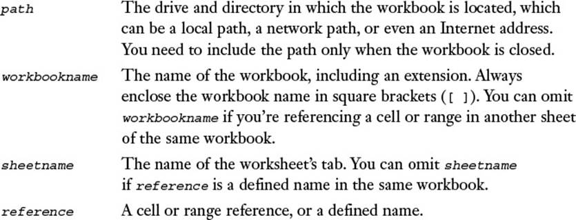
For example, if you close the 2017 Budget workbook, Excel automatically changes the external reference shown in Figure 3.11 to this (depending on the actual path of the file):
='C:\Users\Paul\Documents\[2017 Budget.xlsx]Details'!$R$7
Note
You need the single quotation marks around the path, workbook name, and sheet name only if the workbook is closed or if the path, workbook, or sheet name contains spaces. If in doubt, include the single quotation marks anyway; Excel happily ignores them if they’re not required.
Updating Links
The purpose of a link is to avoid duplicating formulas and data in multiple worksheets. If one workbook contains the information you need, you can use a link to reference the data without re-creating it in another workbook.
To be useful, however, the data in the dependent workbook should always reflect what actually is in the source workbook. You can make sure of this by updating the link, as explained here:
![]() If both the source and the dependent workbooks are open, Excel automatically updates the link whenever the data in the source file changes.
If both the source and the dependent workbooks are open, Excel automatically updates the link whenever the data in the source file changes.
![]() If the source workbook is open when you open the dependent workbook, Excel automatically updates the links again.
If the source workbook is open when you open the dependent workbook, Excel automatically updates the links again.
![]() If the source workbook is closed when you open the dependent workbook, Excel displays a security warning in the information bar, which tells you that automatic updating of links has been disabled. In this case, click Enable Content.
If the source workbook is closed when you open the dependent workbook, Excel displays a security warning in the information bar, which tells you that automatic updating of links has been disabled. In this case, click Enable Content.
Tip
If you always trust the links in your workbooks (that is, if you never deal with third-party workbooks or any other workbooks from sources you don’t completely trust), you can configure Excel to always update links automatically. To begin, select File, Options, click Trust Center, and then click Trust Center Settings. In the Trust Center dialog box, click External Content and then click to select the Enable Automatic Update for All Workbook Links option. Click OK and then click OK again.
![]() If you didn’t update a link when you opened the dependent document, you can update it any time by choosing Data, Edit Links. In the Edit Links dialog box that appears (see Figure 3.12), click the link and then click Update Values.
If you didn’t update a link when you opened the dependent document, you can update it any time by choosing Data, Edit Links. In the Edit Links dialog box that appears (see Figure 3.12), click the link and then click Update Values.
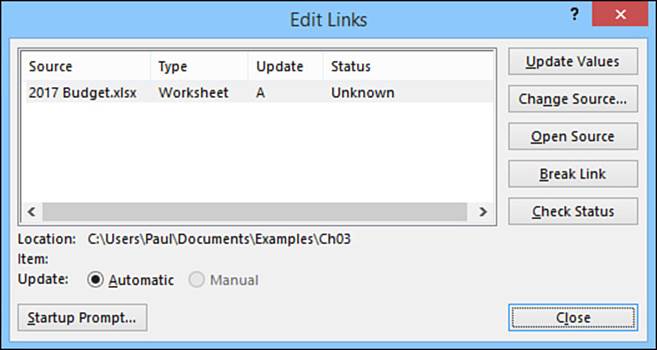
Figure 3.12 Use the Edit Links dialog box to update the linked data in the source workbook.
Changing the Link Source
If the name of the source document changes, you’ll need to edit the link to keep the data up to date. You can edit the external reference directly, or you can change the source by following these steps:
1. With the dependent workbook active, select Data, Edit Links to display the Edit Links dialog box.
2. Click the link you want to work with.
3. Click Change Source. Excel displays the Change Source dialog box.
4. Find and then select the new source document and then click OK to return to the Edit Links dialog box.
5. Click Close to return to the workbook.
Formatting Numbers, Dates, and Times
One of the best ways to improve the readability of worksheets is to display your data in a format that is logical, consistent, and straightforward. Formatting currency amounts with leading dollar signs, percentages with trailing percent signs, and large numbers with commas are a few of the ways you can improve your spreadsheet style.
This section shows you how to format numbers, dates, and times using Excel’s built-in formatting options. You’ll also learn how to create your own formats to gain maximum control over the appearance of your data.
Numeric Display Formats
When you enter numbers in a worksheet, Excel removes any leading or trailing zeros. For example, if you enter 0123.4500, Excel displays 123.45. The exception to this rule occurs when you enter a number that is wider than the cell. In that case, Excel usually expands the width of the column to fit the number. However, in some cases, Excel tailors the number to fit the cell by rounding off some decimal places. For example, a number such as 123.45678 is displayed as 123.4568. Note that, in this case, the number is changed for display purposes only; Excel still retains the original number internally.
When you create a worksheet, each cell uses this format, known as the General number format, by default. If you want your numbers to appear differently, you can select from among Excel’s seven categories of numeric formats:
![]() Number—The number formats have three components: the number of decimal places, whether the thousands separator (,) is used, and how negative numbers are displayed. For negative numbers, you can display the number with a leading minus sign, in red, surrounded by parentheses, or in red surrounded by parentheses.
Number—The number formats have three components: the number of decimal places, whether the thousands separator (,) is used, and how negative numbers are displayed. For negative numbers, you can display the number with a leading minus sign, in red, surrounded by parentheses, or in red surrounded by parentheses.
Note
Although you can select a number as high as 30 in the Decimal Places spin box, Excel will display only the first 14 decimal places. This applies to percentages as well (see below).
![]() Currency—The currency formats are similar to the number formats, except that the thousands separator is always used, and you have the option of displaying the numbers with a leading dollar sign ($) or some other currency symbol.
Currency—The currency formats are similar to the number formats, except that the thousands separator is always used, and you have the option of displaying the numbers with a leading dollar sign ($) or some other currency symbol.
![]() Accounting—With the accounting formats, you can select the number of decimal places and whether to display a leading dollar sign (or other currency symbol). If you do use a dollar sign, Excel displays it flush left in the cell. All negative entries are displayed surrounded by parentheses.
Accounting—With the accounting formats, you can select the number of decimal places and whether to display a leading dollar sign (or other currency symbol). If you do use a dollar sign, Excel displays it flush left in the cell. All negative entries are displayed surrounded by parentheses.
![]() Percentage—The percentage formats display the number multiplied by 100 with a percent sign (%) to the right of the number. For example, .506 is displayed as 50.6%. You can display up to 14 decimal places.
Percentage—The percentage formats display the number multiplied by 100 with a percent sign (%) to the right of the number. For example, .506 is displayed as 50.6%. You can display up to 14 decimal places.
![]() Fraction—The fraction formats enable you to express decimal quantities as fractions. There are nine fraction formats in all, including displaying the number as halves, quarters, eighths, sixteenths, tenths, and hundredths.
Fraction—The fraction formats enable you to express decimal quantities as fractions. There are nine fraction formats in all, including displaying the number as halves, quarters, eighths, sixteenths, tenths, and hundredths.
![]() Scientific—The scientific formats display the most significant number to the left of the decimal, 2-30 decimal places to the right of the decimal, and then the exponent. So, 123000 is displayed as 1.23E+05.
Scientific—The scientific formats display the most significant number to the left of the decimal, 2-30 decimal places to the right of the decimal, and then the exponent. So, 123000 is displayed as 1.23E+05.
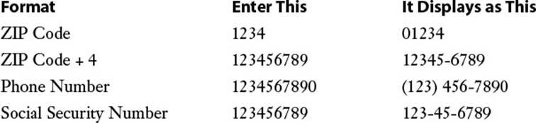
![]() Special—The special formats are a collection designed to take care of special cases. Here’s a list of the special formats, with some examples:
Special—The special formats are a collection designed to take care of special cases. Here’s a list of the special formats, with some examples:
Changing Numeric Formats
The quickest way to format numbers is to specify the format as you enter your data. For example, if you begin a dollar amount with a dollar sign ($), Excel automatically formats the number as currency. Similarly, if you type a percent sign (%) after a number, Excel automatically formats the number as a percentage. Here are a few more examples of this technique. Note that you can enter a negative value using either the negative sign (-) or parentheses.
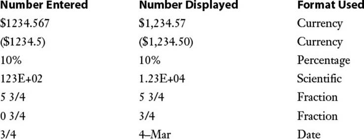
Note
Excel interprets a simple fraction such as 3/4 as a date (March 4, in this case). Always include a leading zero, followed by a space, if you want to enter a simple fraction in the formula bar.
Specifying the numeric format as you enter a number is fast and efficient because Excel guesses the format you want to use. Unfortunately, Excel sometimes guesses wrong (for example, interpreting a simple fraction as a date). In any case, you don’t have access to all the available formats (for example, displaying negative dollar amounts in red). To overcome these limitations, you can select your numeric formats from a list. Here are the steps to follow:
1. Select the cell or range of cells to which you want to apply the new format.
2. Select the Home tab.
3. Pull down the Number Format list. Excel displays its built-in formats, as shown in Figure 3.13. Under the name of each format, Excel shows you how the current cell would be displayed if you chose that format.
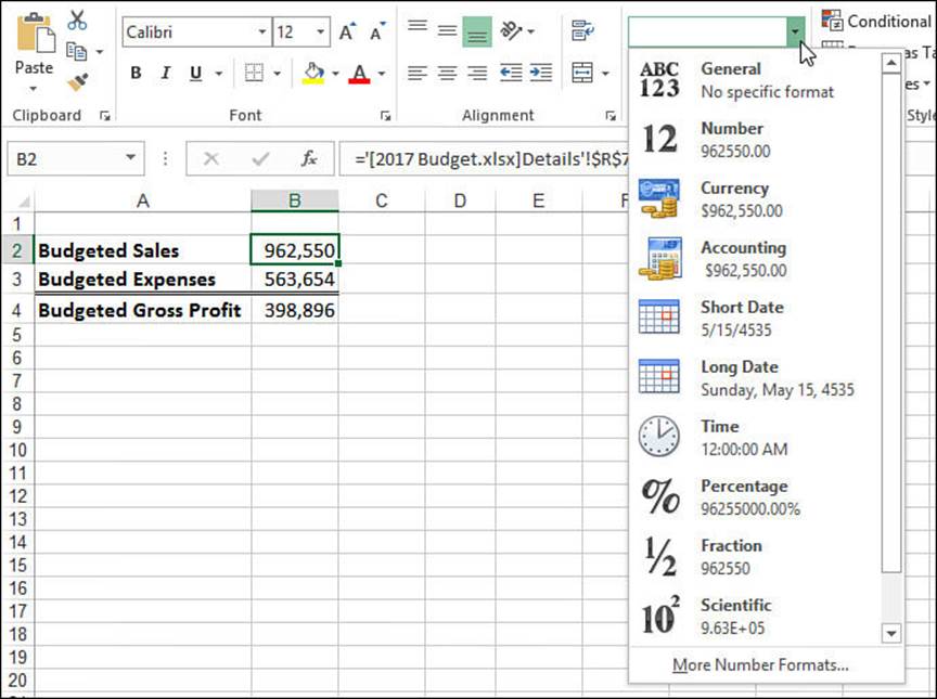
Figure 3.13 On the Home tab, pull down the Number Format list to see all of Excel’s built-in numeric formats.
4. Click the format you want to use.
For more numeric formatting options, use the Number tab of the Format Cells dialog box (or display the Number Format list and select More Number Formats). Select the cell or range and then select Home, Number Format, More Number Formats. (You can also click the Number group’s dialog box launcher or press Ctrl+1.) As you can see in Figure 3.14, when you click a numeric format in the Category list, Excel displays more formatting options, such as the Decimal Places spin box. (The options you see depend on the category you select.) The Sample information box shows a sample of the format applied to the current cell’s contents.
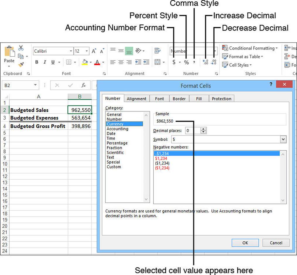
Figure 3.14 When you select a format in the Category list, Excel displays the format’s options.
As an alternative to the Format Cells dialog box, Excel offers several keyboard shortcuts for setting the numeric format. Select the cell or range you want to format and use one of the key combinations listed in Table 3.6.
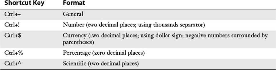
Table 3.6 Shortcut Keys for Selecting Numeric Formats
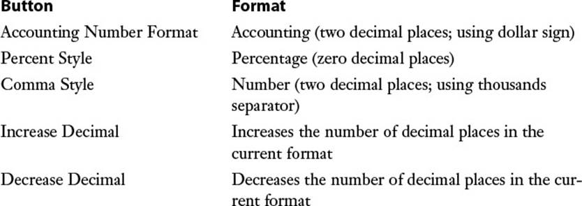
You can use the controls in the Home tab’s Number group as another method of selecting numeric formats. The Number Format list (refer to Figure 3.13) displays all the formats. Here are the other controls that appear in this group:
Customizing Numeric Formats
Excel numeric formats give you lots of control over how your numbers are displayed, but they have their limitations. For example, no built-in format enables you to display a number such as 0.5 without the leading zero or to display temperatures using, for example, the degree symbol.
To overcome these and other limitations, you need to create your own custom numeric formats. You can do this either by editing an existing format or by entering your own from scratch. The formatting syntax and symbols are explained in detail later in this section.
Every Excel numeric format, whether built in or customized, has the following syntax:
positive format;negative format;zero format;text format
The four parts, separated by semicolons, determine how various numbers are presented. The first part defines how a positive number is displayed, the second part defines how a negative number is displayed, the third part defines how zero is displayed, and the fourth part defines how text is displayed. If you leave out one or more of these parts, numbers are controlled as shown here:
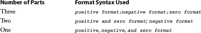
Table 3.7 lists the special symbols you use to define each of these parts.
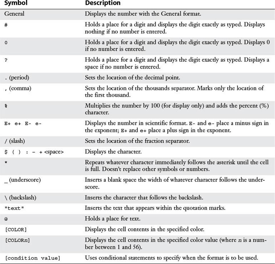
Table 3.7 Numeric Formatting Symbols
Before looking at some examples, let’s run through the basic procedure. To customize a numeric format, select the cell or range you want to format and then follow these steps:
1. Select Home, Number Format, More Number Formats (or press Ctrl+1) and select the Number tab, if it’s not already displayed.
2. In the Category list, click Custom.
3. If you’re editing an existing format, select it in the Type list box.
4. Edit or enter your format code.
5. Click OK. Excel returns you to the worksheet, where you see the custom format applied.
Excel stores each new format definition in the Custom category. If you edited an existing format, the original format is left intact, and the new format is added to the list. You can select the custom formats the same way you select the built-in formats. To use a custom format in other workbooks, you copy a cell containing the format to that workbook. Figure 3.15 shows a dozen examples of custom formats.
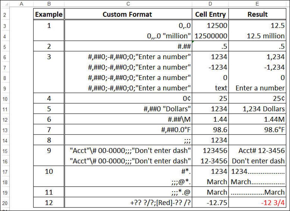
Figure 3.15 Sample custom numeric formats.
Here’s a quick explanation of each example:
![]() Example 1—These formats show how you can reduce a large number to a smaller, more readable one by using the thousands separator. A format such as 0,000.0 would display, for example, 12500 as 12,500.0. If you remove the three zeros between the comma and the decimal (to get the format 0,.0), Excel displays the number as 12.5 (although it still uses the original number in calculations). In essence, you’ve told Excel to express the number in thousands. To express a larger number in millions, you just add a second thousands separator.
Example 1—These formats show how you can reduce a large number to a smaller, more readable one by using the thousands separator. A format such as 0,000.0 would display, for example, 12500 as 12,500.0. If you remove the three zeros between the comma and the decimal (to get the format 0,.0), Excel displays the number as 12.5 (although it still uses the original number in calculations). In essence, you’ve told Excel to express the number in thousands. To express a larger number in millions, you just add a second thousands separator.
![]() Example 2—Use this format when you want to display no leading or trailing zeros.
Example 2—Use this format when you want to display no leading or trailing zeros.
![]() Example 3—These are examples of four-part formats. The first three parts define how Excel should display positive numbers, negative numbers, and zero. The fourth part displays the message “Enter a number” if the user enters text in the cell.
Example 3—These are examples of four-part formats. The first three parts define how Excel should display positive numbers, negative numbers, and zero. The fourth part displays the message “Enter a number” if the user enters text in the cell.
![]() Example 4—In this example, the cents sign (¢) is used after the value. To enter the cents sign, press Alt+0162 on your keyboard’s numeric keypad. (This won’t work if you use the numbers along the top of the keyboard.) Table 3.8 shows some common ANSI characters you can use.
Example 4—In this example, the cents sign (¢) is used after the value. To enter the cents sign, press Alt+0162 on your keyboard’s numeric keypad. (This won’t work if you use the numbers along the top of the keyboard.) Table 3.8 shows some common ANSI characters you can use.
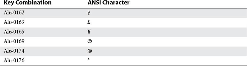
Table 3.8 ANSI Character Key Combinations
![]() Example 5—This example adds the thousands separator and the text string "Dollars" to the format.
Example 5—This example adds the thousands separator and the text string "Dollars" to the format.
![]() Example 6—In this example, an M is appended to any number, which is useful if your spreadsheet unit is megabytes.
Example 6—In this example, an M is appended to any number, which is useful if your spreadsheet unit is megabytes.
![]() Example 7—This example uses the degree symbol (°) to display temperatures.
Example 7—This example uses the degree symbol (°) to display temperatures.
![]() Example 8—The three semicolons used in this example result in no number being displayed (which is useful as a basic method for hiding a sensitive value).
Example 8—The three semicolons used in this example result in no number being displayed (which is useful as a basic method for hiding a sensitive value).
![]() Example 9—This example shows that you can get a number sign (#) to display in your formats by preceding # with a backslash (\).
Example 9—This example shows that you can get a number sign (#) to display in your formats by preceding # with a backslash (\).
![]() Example 10—In this example, you see a trick for creating dot trailers. Recall that the asterisk (*) symbol fills the cell with whatever character follows it. So, creating a dot trailer is a simple matter of adding "*." to the end of the format.
Example 10—In this example, you see a trick for creating dot trailers. Recall that the asterisk (*) symbol fills the cell with whatever character follows it. So, creating a dot trailer is a simple matter of adding "*." to the end of the format.
![]() Example 11—This example shows a similar technique that creates a dot leader. Here, the first three semicolons display nothing; then "*." runs dots from the beginning of the cell up to the text (represented by the @ sign).
Example 11—This example shows a similar technique that creates a dot leader. Here, the first three semicolons display nothing; then "*." runs dots from the beginning of the cell up to the text (represented by the @ sign).
![]() Example 12—This example shows a format that’s useful for entering stock quotations.
Example 12—This example shows a format that’s useful for entering stock quotations.
Hiding Zeros
Worksheets look less cluttered and are easier to read if you hide unnecessary zeros. Excel enables you to hide zeros either throughout an entire worksheet or only in selected cells.
To hide all zeros, select File, Options, click the Advanced tab in the Excel Options dialog box, and scroll down to the Display Options for This Worksheet section. Clear the Show a Zero in Cells That Have Zero Value check box and then click OK.
To hide zeros in selected cells, create a custom format that uses the following format syntax:
positive format;negative format;
The extra semicolon at the end acts as a placeholder for the zero format. Because there’s no definition for a zero value, nothing is displayed. For example, the format $#,##0.00_);($#,##0.00); displays standard dollar values, but it leaves the cell blank if it contains zero.
Tip
If your worksheet contains only integers (no fractions or decimal places), you can use the format #,### to hide zeros.
Using Condition Values
The actions of the formats you’ve seen so far have depended on whether the cell contents were positive, negative, zero, or text. Although this is fine for most applications, sometimes you need to format a cell based on different conditions. For example, you might want only specific numbers, or numbers within a certain range, to take on a particular format. You can achieve this effect by using the [condition value] format symbol. With this symbol, you set up conditional statements using the logical operators =, <, >, <=, >=, and <>, plus the appropriate numbers. You then assign these conditions to each part of your format definition.
For example, suppose you have a worksheet for which the data must be within the range -1,000 to 1,000. To flag numbers outside this range, you set up the following format definition:
[>=1000]"Error: Value >= 1,000";[<=-1000]"Error: Value <= -1,000";0.00
The first part defines the format for numbers greater than or equal to 1,000 (an error message). The second part defines the format for numbers less than or equal to -1,000 (also an error message). The third part defines the format for all other numbers (0.00).
![]() To learn about using Excel’s extensive conditional formatting features, see “Applying Conditional Formatting to a Range,” p. 25.
To learn about using Excel’s extensive conditional formatting features, see “Applying Conditional Formatting to a Range,” p. 25.
Date and Time Display Formats
If you include dates or times in your worksheets, you need to make sure that they’re presented in a readable, unambiguous format. For example, most Americans would interpret the date 8/5/16 as August 5, 2016. However, in some countries, this date would mean May 8, 2016. Similarly, if you use the time 2:45, do you mean a.m. or p.m.? To avoid these kinds of problems, you can use Excel’s built-in date and time formats, listed in Table 3.9.
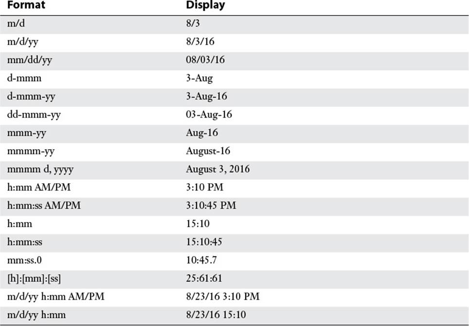
Table 3.9 Excel’s Date and Time Formats
The [h]:[mm]:[ss] format requires a bit of explanation. You use this format when you want to display hours greater than 24 or minutes and seconds greater than 60. For example, suppose that you have an application in which you need to sum several time values (such as the time you’ve spent working on a project). If you add, say, 10:00 and 15:00, Excel normally shows the total as 1:00 (because, by default, Excel restarts times at 0 when they hit 24:00). To display the result properly (that is, as 25:00), use the format [h]:00.
You use the same methods you used for numeric formats to select date and time formats. In particular, you can specify the date and time format as you input your data. For example, entering Jan-16 automatically formats the cell with the mmm-yy format. Also, you can use the following shortcut keys:
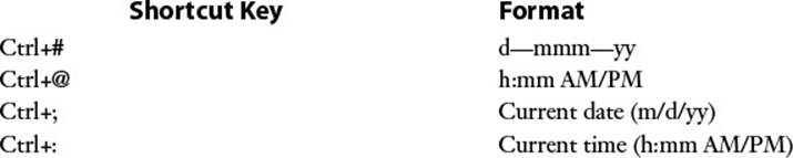
Tip
Excel for the Macintosh uses a different date system than Excel for Windows uses. If you share files between these environments, you need to use Macintosh dates in your Excel for Windows worksheets to maintain the correct dates when you move from one system to another. Select File, Options, click Advanced, scroll down to the When Calculating This Workbook section, and then select the Use 1904 Date System check box.
Customizing Date and Time Formats
Although the built-in date and time formats are fine for most applications, you might need to create your own custom formats. For example, you might want to display the day of the week (for example, Friday). Custom date and time formats generally are simpler to create than custom numeric formats. There are fewer formatting symbols, and you usually don’t need to specify different formats for different conditions. Table 3.10 lists the date and time formatting symbols.
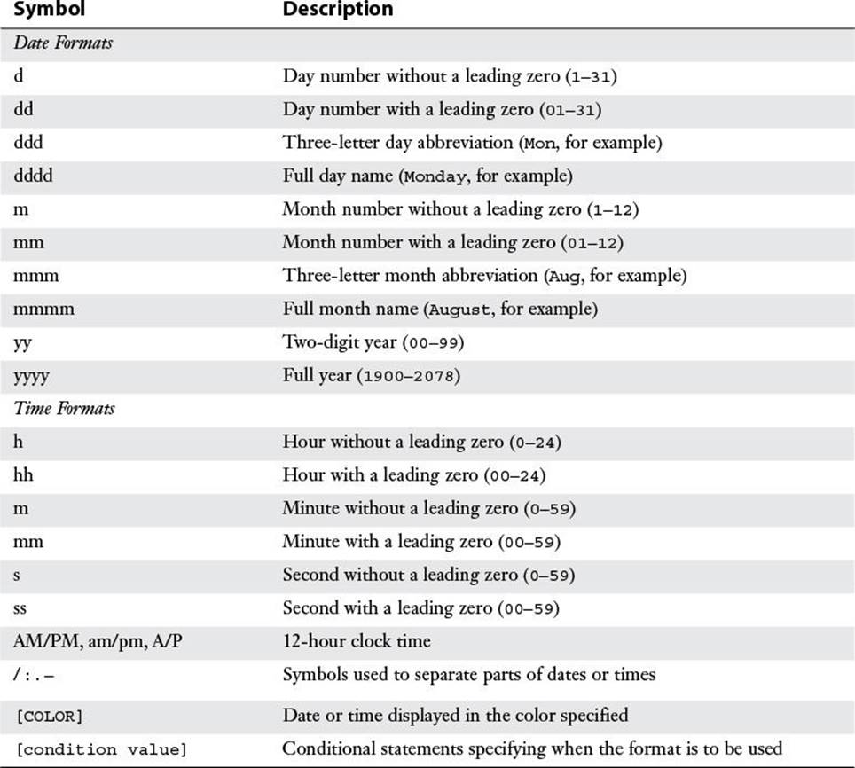
Table 3.10 Date and Time Formatting Symbols
Figure 3.16 shows some examples of custom date and time formats.
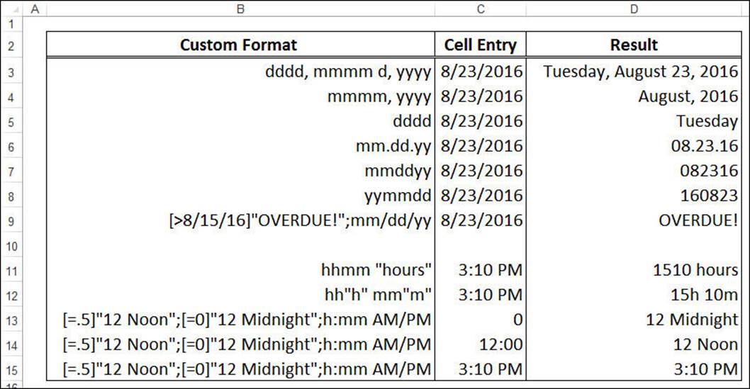
Figure 3.16 Sample custom date and time formats.
Deleting Custom Formats
The best way to become familiar with custom formats is to try your own experiments. Just remember that Excel stores each format you try. If you find that your list of custom formats is getting a bit unwieldy or that it’s cluttered with unused formats, you can delete formats by following the steps outlined here:
1. Select Home, Number Format, More Number Formats.
2. Click the Custom category.
3. Click the format in the Type list box. (Note that you can delete only the formats that were added to Excel’s standard list.)
4. Click Delete. Excel removes the format from the list.
5. To delete other formats, repeat steps 2 through 4.
6. Click OK. Excel returns you to the spreadsheet.
From Here
![]() To learn about conditional formatting, see “Applying Conditional Formatting to a Range,” p. 25.
To learn about conditional formatting, see “Applying Conditional Formatting to a Range,” p. 25.
![]() To learn how to solve formula problems, see Chapter 5, “Troubleshooting Formulas,” p. 111.
To learn how to solve formula problems, see Chapter 5, “Troubleshooting Formulas,” p. 111.
![]() To get details on text formulas and functions, see Chapter 7, “Working with Text Functions,” p. 139.
To get details on text formulas and functions, see Chapter 7, “Working with Text Functions,” p. 139.
![]() If you want to use logical worksheet functions in your comparison formulas, see “Adding Intelligence with Logical Functions,” p. 163.
If you want to use logical worksheet functions in your comparison formulas, see “Adding Intelligence with Logical Functions,” p. 163.
![]() To learn how to create and use data tables, see “Using What-If Analysis,” p. 349.
To learn how to create and use data tables, see “Using What-If Analysis,” p. 349.
All materials on the site are licensed Creative Commons Attribution-Sharealike 3.0 Unported CC BY-SA 3.0 & GNU Free Documentation License (GFDL)
If you are the copyright holder of any material contained on our site and intend to remove it, please contact our site administrator for approval.
© 2016-2026 All site design rights belong to S.Y.A.