Excel 2016 Formulas (2016)

PART VI
Developing Custom Worksheet Functions

Chapter 26
VBA Custom Function Examples

In This Chapter

· Simple custom function examples

· A custom function to determine a cell’s data type

· A custom function to make a single worksheet function act like multiple functions

· A custom function for generating random numbers and selecting cells at random

· Custom functions for calculating sales commissions

· Custom functions for manipulating text

· Custom functions for counting and summing cells

· Custom functions that deal with dates

· A custom function example for returning the last nonempty cell in a column or row

· Custom functions that work with multiple worksheets

· Advanced custom function techniques

This chapter is jam-packed with a variety of useful (or potentially useful) VBA custom worksheet functions. You can use many of the functions as they are written. You may need to modify other functions to meet your particular needs. For maximum speed and efficiency, these Function procedures declare all variables that are used.

Simple Functions

The functions in this section are relatively simple, but they can be very useful. Most of them are based on the fact that VBA can obtain helpful information that’s not normally available for use in a formula.

On the Web

This book’s website contains the workbook simple functions.xlsm that includes all the functions in this section.

Is the cell hidden?

The following CELLISHIDDEN function accepts a single cell argument and returns TRUE if the cell is hidden. A cell is considered a hidden cell if either its row or its column is hidden:

Function CELLISHIDDEN(cell As Range) As Boolean

' Returns TRUE if cell is hidden

Dim UpperLeft As Range

Set UpperLeft = cell.Range("A1")

CELLISHIDDEN = UpperLeft.EntireRow.Hidden Or _

UpperLeft.EntireColumn.Hidden

End Function

Using the functions in this chapter

If you see a function listed in this chapter that you find useful, you can use it in your own workbook. All the Function procedures in this chapter are available at this book's website. Just open the appropriate workbook, activate the VB Editor, and copy and paste the function listing to a VBA module in your workbook. It’s impossible to anticipate every function that you’ll ever need. However, the examples in this chapter cover a variety of topics, so it’s likely that you can locate an appropriate function and adapt the code for your own use.

Returning a worksheet name

The following SHEETNAME function accepts a single argument (a range) and returns the name of the worksheet that contains the range. It uses the Parent property of the Range object. The Parent property returns an object—the worksheet object that contains the Range object:

Function SHEETNAME(rng As Range) As String

' Returns the sheet name for rng

SHEETNAME = rng.Parent.Name

End Function

The following function is a variation on this theme. It does not use an argument; rather, it relies on the fact that a function can determine the cell from which it was called by using Application.Caller:

Function SHEETNAME2() As String

' Returns the sheet name of the cell that contains the function

SHEETNAME2 = Application.Caller.Parent.Name

End Function

In this function, the Caller property of the Application object returns a Range object that corresponds to the cell that contains the function. For example, suppose that you have the following formula in cell A1:

=SHEETNAME2()

When the SHEETNAME2 function is executed, the Application.Caller property returns a Range object corresponding to the cell that contains the function. The Parent property returns the Worksheet object, and the Name property returns the name of the worksheet.

You can use the SHEET function to return a sheet number rather than a sheet name.

Returning a workbook name

The next function, WORKBOOKNAME, returns the name of the workbook. Notice that it uses the Parent property twice. The first Parent property returns a Worksheet object, the second Parent property returns a Workbook object, and the Name property returns the name of the workbook:

Function WORKBOOKNAME() As String

' Returns the workbook name of the cell that contains the function

WORKBOOKNAME = Application.Caller.Parent.Parent.Name

End Function

Returning the application’s name

The following function, although not very useful, carries this discussion of object parents to the next logical level by accessing the Parent property three times. This function returns the name of the Application object, which is always the string Microsoft Excel:

Function APPNAME() As String

' Returns the application name of the cell that contains the function

APPNAME = Application.Caller.Parent.Parent.Parent.Name

End Function

Understanding object parents

Objects in Excel are arranged in a hierarchy. At the top of the hierarchy is the Application object (Excel itself). Excel contains other objects; these objects contain other objects, and so on. The following hierarchy depicts the way a Range object fits into this scheme:

· Application object (Excel)

·  Workbook object

·   Worksheet object

·    Range object

In the lingo of object-oriented programming (OOP), a Range object’s parent is the Worksheet object that contains it. A Worksheet object’s parent is the workbook that contains the worksheet. And a Workbook object’s parent is the Application object. Armed with this knowledge, you can use the Parent property to create a few useful functions.

Returning Excel’s version number

The following function returns Excel's version number. For example, if you use Excel 2016, it returns the text string 16.0:

Function EXCELVERSION() as String

' Returns Excel's version number

EXCELVERSION = Application.Version

End Function

Note that the EXCELVERSION function returns a string, not a value. The following function returns TRUE if the application is Excel 2007 or later (Excel 2007 is version 12). This function uses the VBA Val function to convert the text string to a value:

Function EXCEL2007ORLATER() As Boolean

EXCEL2007ORLATER = Val(Application.Version) >= 12

End Function

Returning cell formatting information

This section contains a number of custom functions that return information about a cell’s formatting. These functions are useful if you need to sort data based on formatting (for example, sorting all bold cells together).

Warning

The functions in this section use the following statement:

Application.Volatile True

This statement causes the function to be reevaluated when the workbook is calculated. You’ll find, however, that these functions don’t always return the correct value. This is because changing cell formatting, for example, does not trigger Excel’s recalculation engine. To force a global recalculation (and update all the custom functions), press Ctrl+Alt +F9.

The following function returns TRUE if its single-cell argument has bold formatting:

Function ISBOLD(cell As Range) As Boolean

' Returns TRUE if cell is bold

Application.Volatile True

ISBOLD = cell.Range("A1").Font.Bold

End Function

The following function returns TRUE if its single-cell argument has italic formatting:

Function ISITALIC(cell As Range) As Boolean

' Returns TRUE if cell is italic

Application.Volatile True

ISITALIC = cell.Range("A1").Font.Italic

End Function

Both of the preceding functions have a slight flaw: they return an error (#VALUE!) if the cell has mixed formatting. For example, it’s possible that only some characters in the cell are bold.

The following function returns TRUE only if all the characters in the cell are bold. If the Bold property of the Font object returns Null (indicating mixed formatting), the If statement generates an error, and the function name is never set to TRUE. The function name was previously set to FALSE, so that’s the value that the function returns:

Function ALLBOLD(cell As Range) As Boolean

' Returns TRUE if all characters in cell are bold

Dim UpperLeft As Range

Application.Volatile True

Set UpperLeft = cell.Range("A1")

ALLBOLD = False

If UpperLeft.Font.Bold Then ALLBOLD = True

End Function

The following FILLCOLOR function returns a value that corresponds to the color of the cell’s interior (the cell’s fill color). If the cell’s interior is not filled, the function returns 16,777,215. The Color property values range from 0 to 16,777,215:

Function FILLCOLOR(cell As Range) As Long

' Returns a value corresponding to the cell's interior color

Application.Volatile True

FILLCOLOR = cell.Range("A1").Interior.Color

End Function

Note

If a cell is part of a table that uses a style, the FILLCOLOR function does not return the correct color. Similarly, a fill color that results from conditional formatting is not returned by this function. In both cases, the function returns 16,777,215.

The following function returns the number format string for a cell:

Function NUMBERFORMAT(cell As Range) As String

' Returns a string that represents

' the cell's number format

Application.Volatile True

NUMBERFORMAT = cell.Range("A1").NumberFormat

End Function

If the cell uses the default number format, the function returns the string General.

Determining a Cell’s Data Type

Excel provides a number of built-in functions that can help determine the type of data contained in a cell. These include ISTEXT, ISNONTEXT, ISLOGICAL, and ISERROR. In addition, VBA includes functions such as ISEMPTY, ISDATE, and ISNUMERIC.

The following function accepts a range argument and returns a string (Blank, Text, Logical, Error, Date, Time, or Value) that describes the data type of the upper-left cell in the range:

Function CELLTYPE(cell As Range) As String

' Returns the cell type of the upper-left cell in a range

Dim UpperLeft As Range

Application.Volatile True

Set UpperLeft = cell.Range("A1")

Select Case True

Case UpperLeft.NumberFormat = "@"

CELLTYPE = "Text"

Case IsEmpty(UpperLeft.Value)

CELLTYPE = "Blank"

Case WorksheetFunction.IsText(UpperLeft)

CELLTYPE = "Text"

Case WorksheetFunction.IsLogical(UpperLeft.Value)

CELLTYPE = "Logical"

Case WorksheetFunction.IsErr(UpperLeft.Value)

CELLTYPE = "Error"

Case IsDate(UpperLeft.Value)

CELLTYPE = "Date"

Case InStr(1, UpperLeft.Text, ":") <> 0

CELLTYPE = "Time"

Case IsNumeric(UpperLeft.Value)

CELLTYPE = "Value"

End Select

End Function

Figure 26.1 shows the CELLTYPE function in use. Column B contains formulas that use the CELLTYPE function with an argument from column A. For example, cell B1 contains the following formula:

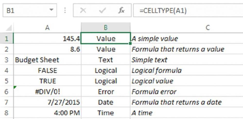
Figure 26.1 The CELLTYPE function returns a string that describes the contents of a cell.

=CELLTYPE(A1)

On the Web

The workbook celltype function.xlsm that demonstrates the CELLTYPE function is available at this book’s website.

A Multifunctional Function

This section demonstrates a technique that may be helpful in some situations—the technique of making a single worksheet function act like multiple functions. The following VBA custom function, named STATFUNCTION, takes two arguments: the range (rng) and the operation (op). Depending on the value of op, the function returns a value computed by using any of the following worksheet functions: AVERAGE, COUNT, MAX, MEDIAN, MIN, MODE, STDEV, SUM, or VAR. For example, you can use this function in your worksheet:

=STATFUNCTION(B1:B24,A24)

The result of the formula depends on the contents of cell A24, which should be a string, such as Average, Count, Max, and so on. You can adapt this technique for other types of functions:

Function STATFUNCTION(rng As Variant, op As String) As Variant

Select Case UCase(op)

Case "SUM"

STATFUNCTION = Application.Sum(rng)

Case "AVERAGE"

STATFUNCTION = Application.Average(rng)

Case "MEDIAN"

STATFUNCTION = Application.Median(rng)

Case "MODE"

STATFUNCTION = Application.Mode(rng)

Case "COUNT"

STATFUNCTION = Application.Count(rng)

Case "MAX"

STATFUNCTION = Application.Max(rng)

Case "MIN"

STATFUNCTION = Application.Min(rng)

Case "VAR"

STATFUNCTION = Application.Var(rng)

Case "STDEV"

STATFUNCTION = Application.StDev(rng)

Case Else

STATFUNCTION = CVErr(xlErrNA)

End Select

End Function

Figure 26.2 shows the STATFUNCTION function that is used in conjunction with a drop-down list generated by Excel’s Data ➜ Data Tools ➜ Data Validation command. The formula in cell C14 is as follows:

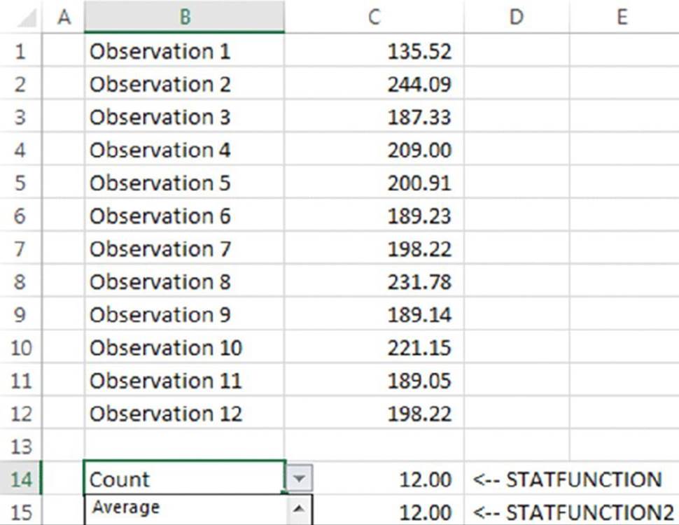
Figure 26.2 Selecting an operation from the list displays the result in cell C14.

=STATFUNCTION(C1:C12,B14)

On the Web

The workbook, statfunction function.xlsm, shown in Figure 26.2, is available on this book’s website.

The following STATFUNCTION2 function is a much simpler approach that works exactly like the STATFUNCTION function. It uses the Evaluate method to evaluate an expression:

Function STATFUNCTION2(rng As Range, op As String) As Double

STATFUNCTION2 = Evaluate(Op & "(" & _

rng.Address(external:=True) & ")")

End Function

For example, assume that the rng argument is C1:C12 and that the op argument is the string SUM. The expression that is used as an argument for the Evaluate method is this:

SUM(C1:C12)

The Evaluate method evaluates its argument and returns the result. In addition to being much shorter, a benefit of this version of STATFUNCTION is that it’s not necessary to list all the possible functions.

Note

Note that the Address property has an argument: external:=True. That argument controls the way the address is returned. The default value, FALSE, returns a simple range address. When the external argument is TRUE, the address includes the workbook name and worksheet name. This allows the function to use a range that’s on a different worksheet or even workbook.

Worksheet function data types

You may have noticed some differences in the data types used for functions and arguments so far. For instance, in STATFUNCTION, the variable rng was declared as a Variant, whereas the same variable was declared as a Range in STATFUNCTION2. Also, the former's return value was declared as a Variant, whereas the latter’s is a Double data type.

Data types are two-edged swords. They can be used to limit the type of data that can be passed to, or returned from, a function, but they can also reduce the flexibility of the function. Using Variant data types maximizes flexibility but may slow execution speed a bit.

One of the possible return values of STATFUNCTION is an error in the Case Else section of the Select Case statement. That means that the function can return a Double data type or an Error. The most restrictive data type that can hold both an Error and aDouble is a Variant (which can hold anything), so the function is typed as a Variant. On the other hand, STATFUNCTION2 does not have a provision continued for returning an error, so it’s typed as the more restrictive Double data type. Numeric data in cells is treated as a Double even if it looks like an Integer.

The rng arguments are also typed differently. In STATFUNCTION2, the Address property of the Range object is used. Because of this, you must pass a Range to the function, or it will return an error. However, there is nothing in STATFUNCTION that forces rng to be aRange. By declaring rng as a Variant, the user has the flexibility to provide inputs in other ways. Excel happily tries to convert whatever it’s given into something it can use. If it can’t convert it, the result is surely an error. A user can enter the following formula:

=STATFUNCTION({123.45,643,893.22},"Min")

Neither argument is a cell reference, but Excel doesn’t mind. It can find the minimum of an array constant as easily as a range of values. It works the other way, too, as in the case of the second argument. If a cell reference is supplied, Excel tries to convert it to a String and has no problem doing so.

In general, you should use the most restrictive data types possible for your situation while providing for the most user flexibility.

Generating Random Numbers

This section presents functions that deal with random numbers. One generates random numbers that don’t change. The other selects a cell at random from a range.

On the Web

The functions in this section are available at this book’s website. The filename is random functions.xlsm.

Generating random numbers that don’t change

You can use the Excel RAND function to quickly fill a range of cells with random values. But, as you may have discovered, the RAND function generates a new random number whenever the worksheet is recalculated. If you prefer to generate random numbers that don’t change with each recalculation, use the following STATICRAND Function procedure:

Function STATICRAND() As Double

' Returns a random number that doesn't

' change when recalculated

STATICRAND = Rnd

End Function

The STATICRAND function uses the VBA Rnd function, which, like Excel’s RAND function, returns a random number between 0 and 1. When you use STATICRAND, however, the random numbers don’t change when the sheet is calculated.

Note

Pressing F9 does not generate new values from the STATICRAND function, but pressing Ctrl+Alt+F9 (Excel’s “global recalc” key combination) does.

Following is another version of the function that returns a random integer within a specified range of values:

Function STATICRANDBETWEEN(lo As Long, hi As Long) As Long

' Returns a random integer that doesn't change when recalculated

STATICRANDBETWEEN = Int((hi – lo + 1) * Rnd + lo)

End Function

For example, if you want to generate a random integer between 1 and 1,000, you can use a formula such as this:

=STATICRANDBETWEEN(1,1000)

Controlling function recalculation

When you use a custom function in a worksheet formula, when is it recalculated?

Custom functions behave like Excel’s built-in worksheet functions. Normally, a custom function is recalculated only when it needs to be recalculated—that is, when you modify any of a function’s arguments—but you can force functions to recalculate more frequently. Adding the following statement to a Function procedure makes the function recalculate whenever the workbook is recalculated:

Application.Volatile True

The Volatile method of the Application object has one argument (either True or False). Marking a Function procedure as “volatile” forces the function to be calculated whenever calculation occurs in any cell in the worksheet.

For example, the custom STATICRAND function presented in this chapter can be changed to emulate the Excel RAND() function by using the Volatile method, as follows:

Function NONSTATICRAND()

' Returns a random number that

' changes when the sheet is recalculated

Application.Volatile True

NONSTATICRAND = Rnd

End Function

Using the False argument of the Volatile method causes the function to be recalculated only when one or more of its arguments change. (If a function has no arguments, this method has no effect.) By default, all custom functions work as if they include an Application.Volatile False statement.

Selecting a cell at random

The following function, named DRAWONE, randomly chooses one cell from an input range and returns the cell’s contents:

Function DRAWONE(rng As Variant) As Double

' Chooses one cell at random from a range

DRAWONE = rng(Int((rng.Count) * Rnd + 1))

End Function

If you use this function, you’ll find that it is not recalculated when the worksheet is calculated. In other words, the function is not volatile. (For more information about controlling recalculation, see the previous sidebar, “Controlling function recalculation.” You can make the function volatile by adding the following statement:

Application.Volatile True

After doing so, the DRAWONE function displays a new random cell value whenever the sheet is calculated.

A more general function, one that accepts array constants as well as ranges, is shown here:

Function DRAWONE2(rng As Variant) As Variant

' Chooses one value at random from an array

Dim ArrayLen As Long

If TypeName(rng) = "Range" Then

DRAWONE2 = rng(Int((rng.Count) * Rnd + 1)).Value

Else

ArrayLen = UBound(rng) – LBound(rng) + 1

DRAWONE2 = rng(Int(ArrayLen * Rnd + 1))

End If

End Function

This function uses the VBA built-in TypeName function to determine whether the argument passed is a Range. If not, it’s assumed to be an array. Following is a formula that uses the DRAWONE2 function. This formula returns a text string that corresponds to a suit in a deck of cards:

=DRAWONE2({"Clubs","Hearts","Diamonds","Spades"})

Following is a formula that has the same result, written using Excel’s built-in functions:

=CHOOSE(RANDBETWEEN(1,4),"Clubs","Hearts","Diamonds","Spades")

We present two additional functions that deal with randomization later in this chapter (see the “Advanced Function Techniques” section).

Calculating Sales Commissions

Sales managers often need to calculate the commissions earned by their sales forces. The calculations in the function example presented here are based on a sliding scale: employees who sell more earn a higher commission rate (see Table 26.1). For example, a salesperson with sales between $10,000 and $19,999 qualifies for a commission rate of 10.5%.

Table 26.1 Commission Rates for Monthly Sales

You can calculate commissions for various sales amounts entered into a worksheet in several ways. You can use a complex formula with nested IF functions, such as the following:

=IF(A1<0,0,IF(A1<10000,A1*0.08,IF(A1<20000,A1*0.105,

IF(A1<40000,A1*0.12,A1*0.14))))

This may not be the best approach for a couple of reasons. First, the formula is overly complex, thus making it difficult to understand. Second, the values are hard-coded into the formula, thus making the formula difficult to modify.

A better approach is to use a lookup table function to compute the commissions. For example:

=VLOOKUP(A1,Table,2)*A1

Using VLOOKUP is a good alternative, but it may not work if the commission structure is more complex. (See the “A function for a simple commission structure” section for more information.) Yet another approach is to create a custom function.

A function for a simple commission structure

The following COMMISSION function accepts a single argument (sales) and computes the commission amount:

Function COMMISSION(Sales As Double) As Double

' Calculates sales commissions

Const Tier1 As Double = 0.08

Const Tier2 As Double = 0.105

Const Tier3 As Double = 0.12

Const Tier4 As Double = 0.14

Select Case Sales

Case Is >= 40000

COMMISSION = Sales * Tier4

Case Is >= 20000

COMMISSION = Sales * Tier3

Case Is >= 10000

COMMISSION = Sales * Tier2

Case Is < 10000

COMMISSION = Sales * Tier1

End Select

End Function

The following worksheet formula, for example, returns 3,000. (The sales amount—25,000—qualifies for a commission rate of 12%.)

=COMMISSION(25000)

This function is easy to understand and maintain. It uses constants to store the commission rates as well as a Select Case structure to determine which commission rate to use.

Note

When a Select Case structure is evaluated, program control exits the Select Case structure when the first true Case is encountered.

A function for a more complex commission structure

If the commission structure is more complex, you may need to use additional arguments for your COMMISSION function. Imagine that the aforementioned sales manager implements a new policy to help reduce turnover: the total commission paid increases by 1 percent for each year that a salesperson stays with the company.

The following is a modified COMMISSION function (named COMMISSION2). This function now takes two arguments: the monthly sales (sales) and the number of years employed (years):

Function COMMISSION2(Sales As Double, Years As Long) As Double

' Calculates sales commissions based on

' years in service

Const Tier1 As Double = 0.08

Const Tier2 As Double = 0.105

Const Tier3 As Double = 0.12

Const Tier4 As Double = 0.14

Select Case Sales

Case Is >= 40000

COMMISSION2 = Sales * Tier4

Case Is >= 20000

COMMISSION2 = Sales * Tier3

Case Is >= 10000

COMMISSION2 = Sales * Tier2

Case Is < 10000

COMMISSION2 = Sales * Tier1

End Select

COMMISSION2 = COMMISSION2 + (COMMISSION2 * Years / 100)

End Function

Figure 26.3 shows the COMMISSION2 function in use. Here’s the formula in cell D2: =COMMISSION2(B2,C2)

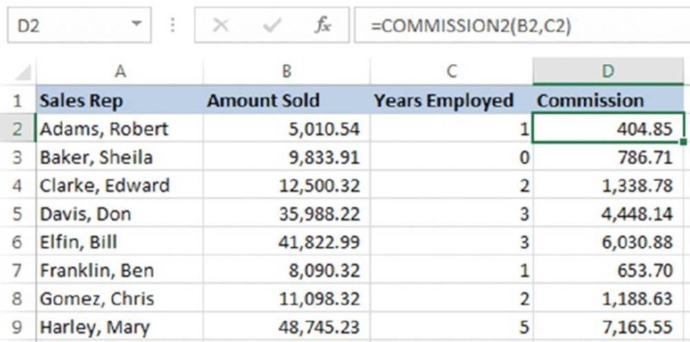
Figure 26.3 Calculating sales commissions based on sales amount and years employed.

The workbook, commission function.xlsm, shown in Figure 26.3, is available at this book’s website.

Text Manipulation Functions

Text strings can be manipulated with functions in a variety of ways, including reversing the display of a text string, scrambling the characters in a text string, or extracting specific characters from a text string. This section offers a number of function examples that manipulate text strings.

On the Web

This book’s website contains a workbook named text manipulation functions.xlsm that demonstrates all the functions in this section.

Reversing a string

The following REVERSETEXT function returns the text in a cell backward:

Function REVERSETEXT(text As String) As String

' Returns its argument, reversed

REVERSETEXT = StrReverse(text)

End Function

This function simply uses the VBA StrReverse function. The following formula, for example, returns tfosorciM:

=REVERSETEXT("Microsoft")

Scrambling text

The following function returns the contents of its argument with the characters randomized. For example, using Microsoft as the argument may return oficMorts or some other random permutation:

Function SCRAMBLE(text As Variant) As String

' Scrambles its string argument

Dim TextLen As Long

Dim i As Long

Dim RandPos As Long

Dim Temp As String

Dim Char As String * 1

If TypeName(text) = "Range" Then

Temp = text.Range("A1").text

ElseIf IsArray(text) Then

Temp = text(LBound(text))

Else

Temp = text

End If

TextLen = Len(Temp)

For i = 1 To TextLen

Char = Mid(Temp, i, 1)

RandPos = WorksheetFunction.RandBetween(1, TextLen)

Mid(Temp, i, 1) = Mid(Temp, RandPos, 1)

Mid(Temp, RandPos, 1) = Char

Next i

SCRAMBLE = Temp

End Function

This function loops through each character and then swaps it with another character in a randomly selected position.

You may be wondering about the use of Mid. Note that when Mid is used on the right side of an assignment statement, it is a function. However, when Mid is used on the left side of the assignment statement, it is a statement. Consult the Help system for more information about Mid.

Returning an acronym

The ACRONYM function returns the first letter (in uppercase) of each word in its argument. For example, the following formula returns IBM:

=ACRONYM("International Business Machines")

The listing for the ACRONYM Function procedure follows:

Function ACRONYM(text As String) As String

' Returns an acronym for text

Dim TextLen As Long

Dim i As Long

text = Application.Trim(text)

TextLen = Len(text)

ACRONYM = Left(text, 1)

For i = 2 To TextLen

If Mid(text, i, 1) = " " Then

ACRONYM = ACRONYM & Mid(text, i + 1, 1)

End If

Next i

ACRONYM = UCase(ACRONYM)

End Function

This function uses the Excel TRIM function to remove any extra spaces from the argument. The first character in the argument is always the first character in the result. The For-Next loop examines each character. If the character is a space, the character after the space is appended to the result. Finally, the result converts to uppercase by using the VBA UCase function.

Does the text match a pattern?

The following function returns TRUE if a string matches a pattern composed of text and wildcard characters. The ISLIKE function is remarkably simple and is essentially a wrapper for the useful VBA Like operator:

Function ISLIKE(text As String, pattern As String) As Boolean

' Returns true if the first argument is like the second

ISLIKE = text Like pattern

End Function

The supported wildcard characters are as follows:

The following formula returns TRUE because the question mark (?) matches any single character. If the first argument were “Unit12”, the function would return FALSE:

=ISLIKE("Unit1","Unit?")

The function also works with values. The following formula, for example, returns TRUE if cell A1 contains a value that begins with 1 and has exactly three numeric digits:

=ISLIKE(A1,"1##")

The following formula returns TRUE because the first argument is a single character contained in the list of characters specified in the second argument:

=ISLIKE("a","[aeiou]")

If the character list begins with an exclamation point (!), the comparison is made with characters not in the list. For example, the following formula returns TRUE because the first argument is a single character that does not appear in the second argument’s list:

=ISLIKE("g","[!aeiou]")

To match one of the special characters from the previous table, put that character in brackets. This formula returns TRUE because the pattern is looking for three consecutive question marks. The question marks in the pattern are in brackets, so they no longer represent a single character:

=ISLIKE("???","[?][?][?]")

The Like operator is versatile. For complete information about the VBA Like operator, consult the Help system.

Does a cell contain a particular word?

What if you need to determine whether a particular word is contained in a string? Excel’s FIND function can determine whether a text string is contained in another text string. For example, the formula that follows returns 5, the character position of rate in the string The rate has changed:

=FIND("rate","The rate has changed")

The following formula also returns 5:

=FIND("rat","The rate has changed")

However, Excel provides no way to determine whether a particular word is contained in a string. Here’s a VBA function that returns TRUE if the second argument is contained in the first argument:

Function EXACTWORDINSTRING(Text As String, Word As String) As Boolean

EXACTWORDINSTRING = " " & UCase(Text) & _

" " Like "*[!A–Z]" & UCase(Word) & "[!A–Z]*"

End Function

Figure 26.4 shows this function in use. Column A contains the text used as the first argument, and column B contains the text used as the second argument. Cell C1 contains this formula, which was copied down the column: =EXACTWORDINSTRING(A1,B1)

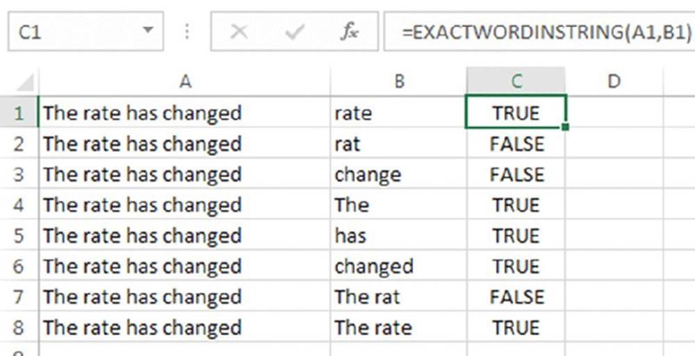
Figure 26.4 A VBA function that determines whether a particular word is contained in a string.

Note

Thanks to Rick Rothstein for suggesting this function, which is much more efficient than our original function.

On the Web

A workbook that demonstrates the EXACTWORDINSTRING function is available on this book’s website. The filename is exact word.xlsm.

Does a cell contain text?

A number of Excel’s worksheet functions are at times unreliable when dealing with text in a cell. For example, the ISTEXT function returns FALSE if its argument is a number that’s formatted as Text. The following CELLHASTEXT function returns TRUE if the range argument contains text or contains a value formatted as Text:

Function CELLHASTEXT(cell As Range) As Boolean

' Returns TRUE if cell contains a string

' or cell is formatted as Text

Dim UpperLeft as Range

CELLHASTEXT = False

Set UpperLeft = cell.Range("A1")

If UpperLeft.NumberFormat = "@" Then

CELLHASTEXT = True

Exit Function

End If

If Not IsNumeric(UpperLeft.Value) Then

CELLHASTEXT = True

Exit Function

End If

End Function

The following formula returns TRUE if cell A1 contains a text string or if the cell is formatted as Text:

=CELLHASTEXT(A1)

Extracting the nth element from a string

The EXTRACTELEMENT function is a custom worksheet function that extracts an element from a text string based on a specified separator character. Assume that cell A1 contains the following text:

123-456-789-9133-8844

For example, the following formula returns the string 9133, which is the fourth element in the string. The string uses a hyphen (-) as the separator:

=EXTRACTELEMENT(A1,4,"-")

The EXTRACTELEMENT function uses three arguments:

§ txt: The text string from which you’re extracting. This can be a literal string or a cell reference.

§ n: An integer that represents the element to extract.

§ separator: A single character used as the separator.

Note

If you specify a space as the Separator character, multiple spaces are treated as a single space, which is almost always what you want. If n exceeds the number of elements in the string, the function returns an empty string.

The VBA code for the EXTRACTELEMENT function follows:

Function EXTRACTELEMENT(Txt As String, n As Long,

Separator As String) As String

' Returns the <i>n</i>th element of a text string, where the

' elements are separated by a specified separator character

Dim AllElements As Variant

AllElements = Split(Txt, Separator)

EXTRACTELEMENT = AllElements(n – 1)

End Function

This function uses the VBA Split function, which returns a variant array that contains each element of the text string. This array begins with 0 (not 1), so using n–1 references the desired element.

Spelling out a number

The SPELLDOLLARS function returns a number spelled out in text—as on a check. For example, the following formula returns the string One hundred twenty-three and 45/100 dollars:

=SPELLDOLLARS(123.45)

Figure 26.5 shows some additional examples of the SPELLDOLLARS function. Column C contains formulas that use the function. For example, the formula in C1 is

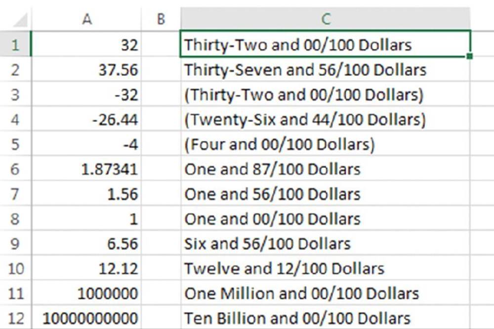
Figure 26.5 Examples of the SPELLDOLLARS function.

=SPELLDOLLARS(A1)

Note that negative numbers are spelled out and enclosed in parentheses.

On the Web

The SPELLDOLLARS function is too lengthy to list here, but you can view the complete listing in spelldollars function.xlsm at this book’s website.

Counting Functions

Chapter 7, “Counting and Summing Techniques,” contains many formula examples to count cells based on various criteria. If you can’t arrive at a formula-based solution for a counting problem, you can probably create a custom function. This section contains three functions that perform counting.

On the Web

This book’s website contains the workbook counting functions.xlsm that demonstrates the functions in this section.

Counting pattern-matched cells

The COUNTIF function accepts limited wildcard characters in its criteria: the question mark and the asterisk, to be specific. If you need more robust pattern matching, you can use the LIKE operator in a custom function:

Function COUNTLIKE(rng As Range, pattern As String) As Long

' Count the cells in a range that match a pattern

Dim cell As Range

Dim cnt As Long

For Each cell In rng.Cells

If cell.Text Like pattern Then cnt = cnt + 1

Next cell

COUNTLIKE = cnt

End Function

The following formula counts the number of cells in B4:B11 that contain the letter e:

=COUNTLIKE(B4:B11,"*[eE]*")

Counting sheets in a workbook

The following countsheets function accepts no arguments and returns the number of sheets in the workbook from where it’s called:

Function COUNTSHEETS() As Long

COUNTSHEETS = Application.Caller.Parent.Parent.Sheets.Count

End Function

This function uses Application.Caller to get the range where the formula was entered. Then it uses two Parent properties to go to the sheet and the workbook. Once at the workbook level, the Count property of the Sheets property is returned. The count includes worksheets and chart sheets.

Counting words in a range

The WORDCOUNT function accepts a range argument and returns the number of words in that range:

Function WORDCOUNT(rng As Range) As Long

' Count the words in a range of cells

Dim cell As Range

Dim WdCnt As Long

Dim tmp As String

For Each cell In rng.Cells

tmp = Application.Trim(cell.Value)

If WorksheetFunction.IsText(tmp) Then

WdCnt = WdCnt + (Len(tmp) – _

Len(Replace(tmp, " ", "")) + 1)

End If

Next cell

WORDCOUNT = WdCnt

End Function

We use a variable, tmp, to store the cell contents with extra spaces removed. Looping through the cells in the supplied range, the ISTEXT worksheet function is used to determine whether the cell has text. If it does, the number of spaces are counted and added to the total. Then one more space is added because a sentence with three spaces has four words. Spaces are counted by comparing the length of the text string with the length after the spaces have been removed with the VBA Replace function.

Date Functions

Chapter 6, “Working with Dates and Times,” presents a number of useful Excel functions and formulas for calculating dates, times, and time periods by manipulating date and time serial values. This section presents additional functions that deal with dates.

On the Web

This book’s website contains a workbook, date functions.xlsm, that demonstrates the functions presented in this section.

Calculating the next Monday

The following NEXTMONDAY function accepts a date argument and returns the date of the following Monday:

Function NEXTMONDAY(d As Date) As Date

NEXTMONDAY = d + 8 – WeekDay(d, vbMonday)

End Function

This function uses the VBA WeekDay function, which returns an integer that represents the day of the week for a date (1 = Sunday, 2 = Monday, and so on). It also uses a predefined constant, vbMonday.

The following formula returns 12/28/2015, which is the first Monday after Christmas Day, 2015 (which is a Friday):

=NEXTMONDAY(DATE(2015,12,25))

Note

The function returns a date serial number. You need to change the number format of the cell to display this serial number as an actual date.

If the argument passed to the NEXTMONDAY function is a Monday, the function returns the following Monday. If you prefer the function to return the same Monday, use this modified version:

Function NEXTMONDAY2(d As Date) As Date

If WeekDay(d) = vbMonday Then

NEXTMONDAY2 = d

Else

NEXTMONDAY2 = d + 8 – WeekDay(d, vbMonday)

End If

End Function

Calculating the next day of the week

The following NEXTDAY function is a variation on the NEXTMONDAY function. This function accepts two arguments: a date and an integer between 1 and 7 that represents a day of the week (1 = Sunday, 2 = Monday, and so on). The NEXTDAY function returns the date for the next specified day of the week:

Function NEXTDAY(d As Date, day As Integer) As Variant

' Returns the next specified day

' Make sure day is between 1 and 7

If day < 1 Or day > 7 Then

NEXTDAY = CVErr(xlErrNA)

Else

NEXTDAY = d + 8 – WeekDay(d, day)

End If

End Function

The NEXTDAY function uses an If statement to ensure that the day argument is valid (that is, between 1 and 7). If the day argument is not valid, the function returns #N/A. Because the function can return a value other than a date, it is declared as type Variant.

Which week of the month?

The following MONTHWEEK function returns an integer that corresponds to the week of the month for a date:

Function MONTHWEEK(d As Date) As Variant

' Returns the week of the month for a date

Dim FirstDay As Integer

' Check for valid date argument

If Not IsDate(d) Then

MONTHWEEK = CVErr(xlErrNA)

Exit Function

End If

' Get first day of the month

FirstDay = WeekDay(DateSerial(Year(d), Month(d), 1))

' Calculate the week number

MONTHWEEK = Application.RoundUp((FirstDay + day(d) – 1) / 7, 0)

End Function

Working with dates before 1900

Many users are surprised to discover that Excel can’t work with dates prior to the year 1900. To correct this deficiency, we created a series of extended date functions. These functions enable you to work with dates in the years 0100 through 9999.

The extended date functions follow:

§ XDATE(y,m,d,fmt): Returns a date for a given year, month, and day. As an option, you can provide a date formatting string.

§ XDATEADD(xdate1,days,fmt): Adds a specified number of days to a date. As an option, you can provide a date formatting string.

§ XDATEDIF(xdate1,xdate2): Returns the number of days between two dates.

§ XDATEYEARDIF(xdate1,xdate2): Returns the number of full years between two dates (useful for calculating ages).

§ XDATEYEAR(xdate1): Returns the year of a date.

§ XDATEMONTH(xdate1): Returns the month of a date.

§ XDATEDAY(xdate1): Returns the day of a date.

§ XDATEDOW(xdate1): Returns the day of the week of a date (as an integer between 1 and 7).

Figure 26.6 shows a workbook that uses a few of these functions.

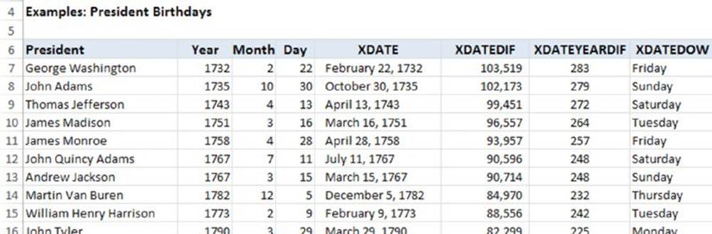
Figure 26.6 Examples of the extended date function.

On the Web

These functions are available on this book’s website, in a file named extended date functions.xlsm. The website also contains a PDF file (extended date functions help.pdf) that describes these functions. The functions are assigned to the Date & Time function category.

Caution

The extended date functions don’t make adjustments for changes made to the calendar in 1582. Consequently, working with dates prior to October 15, 1582, may not yield correct results.

Returning the Last Nonempty Cell in a Column or Row

This section presents two useful functions: LASTINCOLUMN, which returns the contents of the last nonempty cell in a column, and LASTINROW, which returns the contents of the last nonempty cell in a row. Chapter 15, “Performing Magic with Array Formulas,” presents standard formulas for this task, but you may prefer to use a custom function.

On the Web

This book’s website contains last nonempty cell.xlsm, a workbook that demonstrates the functions presented in this section.

Each of these functions accepts a range as its single argument. The range argument can be a column reference (for LASTINCOLUMN) or a row reference (for LASTINROW). If the supplied argument is not a complete column or row reference (such as 3:3 or D:D), the function uses the column or row of the upper-left cell in the range. For example, the following formula returns the contents of the last nonempty cell in column B:

=LASTINCOLUMN(B5)

The following formula returns the contents of the last nonempty cell in row 7:

=LASTINROW(C7:D9)

The LASTINCOLUMN function

The following is the LASTINCOLUMN function:

Function LASTINCOLUMN(rng As Range) As Variant

' Returns the contents of the last nonempty cell in a column

Dim LastCell As Range

With rng.Parent

With .Cells(.Rows.Count, rng.Column)

If Not IsEmpty(.Value) Then

LASTINCOLUMN = .Value

ElseIf IsEmpty(.End(xlUp).Value) Then

LASTINCOLUMN = ""

Else

LASTINCOLUMN = .End(xlUp).Value

End If

End With

End With

End Function

Notice the references to the Parent of the range. This is done to make the function work with arguments that refer to a different worksheet or workbook.

The LASTINROW function

The following is the LASTINROW function:

Function LASTINROW(rng As Range) As Variant

' Returns the contents of the last nonempty cell in a row

With rng.Parent

With .Cells(rng.Row, .Columns.Count)

If Not IsEmpty(.Value) Then

LASTINROW = .Value

ElseIf IsEmpty(.End(xlToLeft).Value) Then

LASTINROW = ""

Else

LASTINROW = .End(xlToLeft).Value

End If

End With

End With

End Function

Cross-Ref

In Chapter 15, we describe array formulas that return the last cell in a column or row.

Multisheet Functions

You may need to create a function that works with data contained in more than one worksheet within a workbook. This section contains two VBA custom functions that enable you to work with data across multiple sheets, including a function that overcomes an Excel limitation when copying formulas to other sheets.

On the Web

This book’s website contains the workbook multisheet functions.xlsm that demonstrates the multisheet functions presented in this section.

Returning the maximum value across all worksheets

If you need to determine the maximum value in a cell (for example, B1) across a number of worksheets, use a formula like this one:

=MAX(Sheet1:Sheet4!B1)

This formula returns the maximum value in cell B1 for Sheet1, Sheet4, and all sheets in between. But what if you add a new sheet (Sheet5) after Sheet4? Your formula does not adjust automatically, so you need to edit it to include the new sheet reference:

=MAX(Sheet1:Sheet5!B1)

The following function accepts a single-cell argument and returns the maximum value in that cell across all worksheets in the workbook. For example, the following formula returns the maximum value in cell B1 for all sheets in the workbook:

=MAXALLSHEETS(B1)

If you add a new sheet, you don't need to edit the formula:

Function MAXALLSHEETS(cell as Range) As Variant

Dim MaxVal As Double

Dim Addr As String

Dim Wksht As Object

Application.Volatile

Addr = cell.Range("A1").Address

MaxVal = –9.9E+307

For Each Wksht In cell.Parent.Parent.Worksheets

If Not Wksht.Name = cell.Parent.Name Or _

Not Addr = Application.Caller.Address Then

If IsNumeric(Wksht.Range(Addr)) Then

If Wksht.Range(Addr) > MaxVal Then _

MaxVal = Wksht.Range(Addr).Value

End If

End If

Next Wksht

If MaxVal = –9.9E+307 Then MaxVal = CVErr(xlErrValue)

MAXALLSHEETS = MaxVal

End Function

The For Each statement uses the following expression to access the workbook:

cell.Parent.Parent.Worksheets

The parent of the cell is a worksheet, and the parent of the worksheet is the workbook. Therefore, the For Each-Next loop cycles among all worksheets in the workbook. The first If statement inside the loop checks whether the cell being checked is the cell that contains the function. If so, that cell is ignored to avoid a circular reference error.

Note

You can easily modify the MAXALLSHEETS function to perform other cross-worksheet calculations: Minimum, Average, Sum, and so on.

The SHEETOFFSET function

A recurring complaint about Excel (including Excel 2016) is its poor support for relative sheet references. For example, suppose that you have a multisheet workbook, and you enter a formula like the following on Sheet2:

=Sheet1!A1+1

This formula works fine. However, if you copy the formula to the next sheet (Sheet3), the formula continues to refer to Sheet1. Or if you insert a sheet between Sheet1 and Sheet2, the formula continues to refer to Sheet1, when most likely, you want it to refer to the newly inserted sheet. In fact, you can’t create formulas that refer to worksheets in a relative manner. However, you can use the SHEETOFFSET function to overcome this limitation.

Following is a VBA Function procedure named SHEETOFFSET:

Function SHEETOFFSET(Offset As Long, Optional cell As Variant)

' Returns cell contents at Ref, in sheet offset

Dim WksIndex As Long, WksNum As Long

Dim wks As Worksheet

Application.Volatile

If IsMissing(cell) Then Set cell = Application.Caller

WksNum = 1

For Each wks In Application.Caller.Parent.Parent.Worksheets

If Application.Caller.Parent.Name = wks.Name Then

SHEETOFFSET = Worksheets(WksNum + Offset)_</p><p>

.Range(cell(1).Address).Value

Exit Function

Else

WksNum = WksNum + 1

End If

Next wks

End Function

The SHEETOFFSET function accepts two arguments:

§ offset: The sheet offset, which can be positive, negative, or 0.

§ cell: (Optional) A single-cell reference. If this argument is omitted, the function uses the same cell reference as the cell that contains the formula.

For more information about optional arguments, see the section “Using optional arguments,” later in this chapter.

The following formula returns the value in cell A1 of the sheet before the sheet that contains the formula:

=SHEETOFFSET(–1,A1)

The following formula returns the value in cell A1 of the sheet after the sheet that contains the formula:

=SHEETOFFSET(1,A1)

Advanced Function Techniques

In this section, we explore some even more advanced functions. The examples in this section demonstrate some special techniques that you can use with your custom functions.

Returning an error value

In some cases, you may want your custom function to return a particular error value. Consider the simple REVERSETEXT function, which we presented earlier in this chapter:

Function REVERSETEXT(text As String) As String

' Returns its argument, reversed

REVERSETEXT = StrReverse(text)

End Function

This function reverses the contents of its single-cell argument (which can be text or a value). If the argument is a multicell range, the function returns #VALUE!

Assume that you want this function to work only with strings. If the argument does not contain a string, you want the function to return an error value (#N/A). You may be tempted to simply assign a string that looks like an Excel formula error value. For example:

REVERSETEXT = "#N/A"

Although the string looks like an error value, it is not treated as such by other formulas that may reference it. To return a real error value from a function, use the VBA CVErr function, which converts an error number to a real error.

Fortunately, VBA has built-in constants for the errors that you want to return from a custom function. These constants are listed here:

§ xlErrDiv0

§ xlErrNA

§ xlErrName

§ xlErrNull

§ xlErrNum

§ xlErrRef

§ xlErrValue

The following is the revised REVERSETEXT function:

Function REVERSETEXT(text As Variant) As Variant

' Returns its argument, reversed

If WorksheetFunction.ISNONTEXT(text) Then

REVERSETEXT = CVErr(xlErrNA)

Else

REVERSETEXT = StrReverse(text)

End If

End Function

First, change the argument from a String data type to a Variant. If the argument’s data type is String, Excel tries to convert whatever it gets (for example, number, Boolean value) to a String and usually succeeds. Next, the Excel ISNONTEXT function is used to determine whether the argument is not a text string. If the argument is not a text string, the function returns the #N/A error. Otherwise, it returns the characters in reverse order.

Note

The data type for the return value of the original REVERSETEXT function was String because the function always returned a text string. In this revised version, the function is declared as a Variant because it can now return something other than a string.

Returning an array from a function

Most functions that you develop with VBA return a single value. It’s possible, however, to write a function that returns multiple values in an array.

Cross-Ref

Part IV, “Array Formulas,” deals with arrays and array formulas. Specifically, these chapters provide examples of a single formula that returns multiple values in separate cells. As you’ll see, you can also create custom functions that return arrays.

VBA includes a useful function called Array. The Array function returns a variant that contains an array. It’s important to understand that the array returned is not the same as a normal array composed of elements of the variant type. In other words, a variant array is not the same as an array of variants.

If you’re familiar with using array formulas in Excel, you have a head start understanding the VBA Array function. You enter an array formula into a cell by pressing Ctrl+Shift+Enter. Excel inserts brackets around the formula to indicate that it’s an array formula. See Chapter 14, “Introducing Arrays,” and Chapter 15 for more details on array formulas.

Note

The lower bound of an array created by using the Array function is, by default, 0. However, the lower bound can be changed if you use an Option Base statement.

The following MONTHNAMES function demonstrates how to return an array from a Function procedure:

Function MONTHNAMES() As Variant

MONTHNAMES = Array( _

"Jan", "Feb", "Mar", "Apr", _

"May", "Jun", "Jul", "Aug", _

"Sep", "Oct", "Nov", "Dec")

End Function

Figure 26.7 shows a worksheet that uses the MONTHNAMES function. You enter the function by selecting A4:L4 and then entering the following formula:

{=MONTHNAMES()}

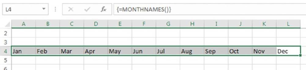
Figure 26.7 The MONTHNAMES function entered as an array formula.

Note

As with any array formula, you must press Ctrl+Shift+Enter to enter the formula. Don’t enter the brackets—Excel inserts the brackets for you.

The MONTHNAMES function, as written, returns a horizontal array in a single row. To display the array in a vertical range in a single column, select the range and enter the following formula:

{=TRANSPOSE(MONTHNAMES())}

Alternatively, you can modify the function to do the transposition. The following function uses the Excel TRANSPOSE function to return a vertical array:

Function VMONTHNAMES() As Variant

VMONTHNAMES = Application.Transpose(Array( _

"Jan", "Feb", "Mar", "Apr", _

"May", "Jun", "Jul", "Aug", _

"Sep", "Oct", "Nov", "Dec"))

End Function

On the Web

The workbook monthnames.xlsm that demonstrates MONTHNAMES and VMONTHNAMES is available at this book’s website.

Returning an array of nonduplicated random integers

The RANDOMINTEGERS function returns an array of nonduplicated integers. This function is intended for use in a multicell array formula. Figure 26.8 shows a worksheet that uses the following formula in the range A3:D12:

{=RANDOMINTEGERS()}

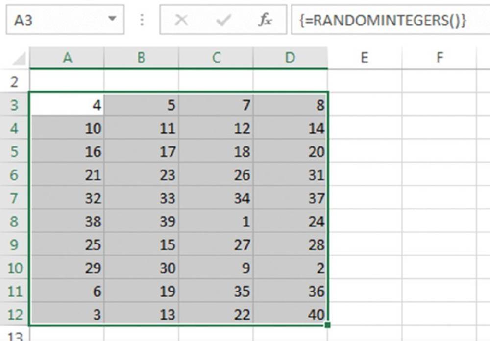
Figure 26.8 An array formula generates nonduplicated consecutive integers, arranged randomly.

This formula was entered into the entire range by using Ctrl+Shift+Enter. The formula returns an array of nonduplicated integers, arranged randomly. Because 40 cells contain the formula, the integers range from 1 to 40. The following is the code for RANDOMINTEGERS:

Function RANDOMINTEGERS()

Dim FuncRange As Range

Dim V() As Integer, ValArray() As Integer

Dim CellCount As Double

Dim i As Integer, j As Integer

Dim r As Integer, c As Integer

Dim Temp1 As Variant, Temp2 As Variant

Dim RCount As Integer, CCount As Integer

Randomize

' Create Range object

Set FuncRange = Application.Caller

' Return an error if FuncRange is too large

CellCount = FuncRange.Count

If CellCount > 1000 Then

RANDOMINTEGERS = CVErr(xlErrNA)

Exit Function

End If

' Assign variables

RCount = FuncRange.Rows.Count

CCount = FuncRange.Columns.Count

ReDim V(1 To RCount, 1 To CCount)

ReDim ValArray(1 To 2, 1 To CellCount)

' Fill array with random numbers

' and consecutive integers

For i = 1 To CellCount

ValArray(1, i) = Rnd

ValArray(2, i) = i

Next i

' Sort ValArray by the random number dimension

For i = 1 To CellCount

For j = i + 1 To CellCount

If ValArray(1, i) > ValArray(1, j) Then

Temp1 = ValArray(1, j)

Temp2 = ValArray(2, j)

ValArray(1, j) = ValArray(1, i)

ValArray(2, j) = ValArray(2, i)

ValArray(1, i) = Temp1

ValArray(2, i) = Temp2

End If

Next j

Next i

' Put the randomized values into the V array

i = 0

For r = 1 To RCount

For c = 1 To CCount

i = i + 1

V(r, c) = ValArray(2, i)

Next c

Next r

RANDOMINTEGERS = V

End Function

On the Web

The workbook random integers function.xlsm containing the RANDOMINTEGERS function is available at this book’s website.

Randomizing a range

The following RANGERANDOMIZE function accepts a range argument and returns an array that consists of the input range in random order:

Function RANGERANDOMIZE(rng)

Dim V() As Variant, ValArray() As Variant

Dim CellCount As Double

Dim i As Integer, j As Integer

Dim r As Integer, c As Integer

Dim Temp1 As Variant, Temp2 As Variant

Dim RCount As Integer, CCount As Integer

Randomize

' Return an error if rng is too large

CellCount = rng.Count

If CellCount > 1000 Then

RANGERANDOMIZE = CVErr(xlErrNA)

Exit Function

End If

' Assign variables

RCount = rng.Rows.Count

CCount = rng.Columns.Count

ReDim V(1 To RCount, 1 To CCount)

ReDim ValArray(1 To 2, 1 To CellCount)

' Fill ValArray with random numbers

' and values from rng

For i = 1 To CellCount

ValArray(1, i) = Rnd

ValArray(2, i) = rng(i)

Next i

' Sort ValArray by the random number dimension

For i = 1 To CellCount

For j = i + 1 To CellCount

If ValArray(1, i) > ValArray(1, j) Then

Temp1 = ValArray(1, j)

Temp2 = ValArray(2, j)

ValArray(1, j) = ValArray(1, i)

ValArray(2, j) = ValArray(2, i)

ValArray(1, i) = Temp1

ValArray(2, i) = Temp2

End If

Next j

Next i

' Put the randomized values into the V array

i = 0

For r = 1 To RCount

For c = 1 To CCount

i = i + 1

V(r, c) = ValArray(2, i)

Next c

Next r

RANGERANDOMIZE = V

End Function

The code closely resembles the code for the RANDOMINTEGERS function. Figure 26.9 shows the function in use. The following array formula, which is in E15:F27, returns the contents of B15:C27 in a random order:

{=RANGERANDOMIZE(B15:C27)}

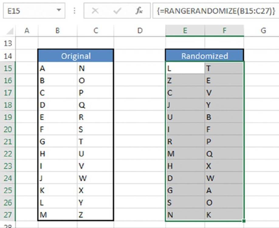
Figure 26.9 The RANGERANDOMIZE function returns the contents of a range, but in a randomized order.

On the Web

The workbook range randomize function.xlsm, which contains the RANGERANDOMIZE function, is available at this book’s website.

Using optional arguments

Many of the built-in Excel worksheet functions use optional arguments. For example, the LEFT function returns characters from the left side of a string. Its official syntax is as follows:

LEFT(text,<i>num_chars</i>)

The first argument is required, but the second is optional. If you omit the optional argument, Excel assumes a value of 1.

Custom functions that you develop in VBA can also have optional arguments. You specify an optional argument by preceding the argument’s name with the keyword Optional. The following is a simple function that returns the user’s name:

Function USER()

USER = Application.UserName

End Function

Suppose that in some cases, you want the user’s name to be returned in uppercase letters. The following function uses an optional argument:

Function USER(Optional UpperCase As Variant) As String

If IsMissing(UpperCase) Then UpperCase = False

If UpperCase = True Then

USER = Ucase(Application.UserName)

Else

USER = Application.UserName

End If

End Function

Note

If you need to determine whether an optional argument was passed to a function, you must declare the optional argument as a variant data type. Then you can use the IsMissing function within the procedure, as demonstrated in this example.

If the argument is FALSE or omitted, the user’s name is returned without changes. If the argument is TRUE, the user’s name converts to uppercase (using the VBA Ucase function) before it is returned. Notice that the first statement in the procedure uses the VBA IsMissing function to determine whether the argument was supplied. If the argument is missing, the statement sets the UpperCase variable to FALSE (the default value).

Optional arguments also allow you to specify a default value in the declaration, rather than testing it with the IsMissing function. The preceding function can be rewritten in this alternate syntax as follows:

Function USER(Optional UpperCase As Boolean = False) As String

If UpperCase = True Then

USER = UCase(Application.UserName)

Else

USER = Application.UserName

End If

End Function

If no argument is supplied, UpperCase is automatically assigned a value of FALSE. This allows you to type the argument appropriately instead of with the generic Variant data type. If you use this method, however, there is no way to tell whether the user omitted the argument or supplied the default argument. Also, the argument will be tagged as optional in the Insert Function dialog.

All the following formulas are valid in either syntax (and the first two have the same effect):

=USER()

=USER(False)

=USER(True)

Using an indefinite number of arguments

Some of the Excel worksheet functions take an indefinite number of arguments. A familiar example is the SUM function, which has the following syntax:

SUM(number1,number2…)

The first argument is required, but you can have as many as 254 additional arguments. Here’s an example of a formula that uses the SUM function with four range arguments:

=SUM(A1:A5,C1:C5,E1:E5,G1:G5)

You can mix and match the argument types. For example, the following example uses three arguments—a range, followed by a value, and finally an expression:

=SUM(A1:A5,12,24*3)

You can create Function procedures that have an indefinite number of arguments. The trick is to use an array as the last (or only) argument, preceded by the keyword ParamArray.

Note

ParamArray can apply only to the last argument in the procedure. It is always a variant data type, and it is always an optional argument (although you don’t use the Optional keyword).

A simple example of arguments

The following is a Function procedure that can have any number of single-value arguments. It simply returns the sum of the arguments:

Function SIMPLESUM(ParamArray arglist() As Variant) As Double

Dim arg as Variant

For Each arg In arglist

SIMPLESUM = SIMPLESUM + arg

Next arg

End Function

The following formula returns the sum of the single-cell arguments:

=SIMPLESUM(A1,A5,12)

The most serious limitation of the SIMPLESUM function is that it does not handle multicell ranges. This improved version does:

Function SIMPLESUM(ParamArray arglist() As Variant) As Double

Dim arg as Variant

Dim cell as Range

For Each arg In arglist

If TypeName(arg) = "Range" Then

For Each cell In arg

SIMPLESUM = SIMPLESUM + cell.Value

Next cell

Else

SIMPLESUM = SIMPLESUM + arg

End If

Next arg

End Function

This function checks each entry in the Arglist array. If the entry is a range, the code uses a For Each-Next loop to sum the cells in the range.

Even this improved version is certainly no substitute for the Excel SUM function. Try it by using various types of arguments, and you’ll see that it fails unless each argument is a value or a range reference. Also, if an argument consists of an entire column, you’ll find that the function is very slow because it evaluates every cell—even the empty ones.

Emulating the Excel SUM function

This section presents a Function procedure called MYSUM. Unlike the SIMPLESUM function listed in the previous section, MYSUM emulates the Excel SUM function perfectly.

Before you look at the code for the MYSUM function, take a minute to think about the Excel SUM function. This versatile function can have any number of arguments (even missing arguments), and the arguments can be numerical values, cells, ranges, text representations of numbers, logical values, and even embedded functions. For example, consider the following formula:

=SUM(A1,5,"6",,TRUE,SQRT(4),B1:B5,{1,3,5})

This formula—which is valid—contains all the following types of arguments, listed here in the order of their presentation:

§ A single cell reference (A1)

§ A literal value (5)

§ A string that looks like a value (“6”)

§ A missing argument

§ A logical value (TRUE)

§ An expression that uses another function (SQRT)

§ A range reference (B1:B5)

§ An array ({1,3,5})

The following is the listing for the MYSUM function that handles all these argument types:

Function MySum(ParamArray args() As Variant) As Variant

' Emulates Excel's SUM function

' Variable declarations

Dim i As Variant

Dim TempRange As Range, cell As Range

Dim ECode As String

Dim m, n

MySum = 0

' Process each argument

For i = 0 To UBound(args)

' Skip missing arguments

If Not IsMissing(args(i)) Then

' What type of argument is it?

Select Case TypeName(args(i))

Case "Range"

' Create temp range to handle full row or column ranges

Set TempRange = Intersect(args(i).Parent.UsedRange, args(i))

For Each cell In TempRange

If IsError(cell) Then

MySum = cell ' return the error

Exit Function

End If

If cell = True Or cell = False Then

MySum = MySum + 0

Else

If IsNumeric(cell) Or IsDate(cell) Then _

MySum = MySum + cell

End If

Next cell

Case "Variant()"

n = args(i)

For m = LBound(n) To UBound(n)

MySum = MySum(MySum, n(m)) 'recursive call

Next m

Case "Null" 'ignore it

Case "Error" 'return the error

MySum = args(i)

Exit Function

Case "Boolean"

' Check for literal TRUE and compensate

If args(i) = "True" Then MySum = MySum + 1

Case "Date"

MySum = MySum + args(i)

Case Else

MySum = MySum + args(i)

End Select

End If

Next i

End Function

On the Web

The workbook sum function emulation.xlsm containing the MYSUM function is available at this book’s website.

Figure 26.10 shows a workbook with various formulas that use SUM (column E) and MYSUM (column G). As you can see, the functions return identical results.

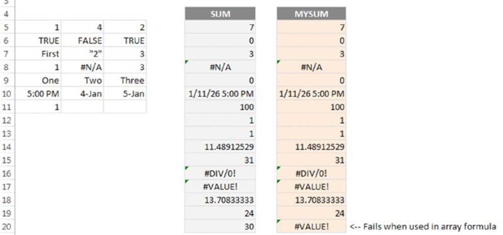
Figure 26.10 Comparing Excel’s SUM function with a custom function.

MYSUM is a close emulation of the SUM function, but it’s not perfect. It cannot handle operations on arrays. For example, this array formula returns the sum of the squared values in range A1:A4:

{=SUM(A:A4^2)}

This formula returns a #VALUE! error:

{=MYSUM(A1:A4^2)}

As you study the code for MYSUM, keep the following points in mind:

§ Missing arguments (determined by the IsMissing function) are simply ignored.

§ The procedure uses the VBA TypeName function to determine the type of argument (Range, Error, or something else). Each argument type is handled differently.

§ For a range argument, the function loops through each cell in the range and adds its value to a running total.

§ The data type for the function is Variant because the function needs to return an error if any of its arguments is an error value.

§ If an argument contains an error (for example, #DIV0!), the MYSUM function simply returns the error—just like the Excel SUM function.

§ The Excel SUM function considers a text string to have a value of 0 unless it appears as a literal argument (that is, as an actual value, not a variable). Therefore, MYSUM adds the cell’s value only if it can be evaluated as a number (VBA’s IsNumeric function is used for this).

§ Dealing with Boolean arguments is tricky. For MYSUM to emulate SUM exactly, it needs to test for a literal TRUE in the argument list and compensate for the difference (that is, add 2 to –1 to get 1).

§ For range arguments, the function uses the Intersect method to create a temporary range that consists of the intersection of the range and the sheet’s used range. This handles cases in which a range argument consists of a complete row or column, which would take forever to evaluate.

You may be curious about the relative speeds of SUM and MYSUM. MYSUM, of course, is much slower, but just how much slower depends on the speed of your system and the formulas themselves. On our system, a worksheet with 5,000 SUM formulas recalculated instantly. After we replaced the SUM functions with MYSUM functions, it took about 8 seconds. MYSUM may be improved a bit, but it can never come close to SUM’s speed.

By the way, we hope you understand that the point of this example is not to create a new SUM function. Rather, it demonstrates how to create custom worksheet functions that look and work like those built into Excel.