Excel 2016 Formulas (2016)

PART II
Leveraging Excel Functions

Chapter 6
Working with Dates and Times

In This Chapter

· An overview of using dates and times in Excel

· Excel’s date-related functions

· Excel’s time-related functions

Beginners often find working with dates and times in Excel to be frustrating. To help avoid this frustration, you’ll need a good understanding of how Excel handles time-based information. This chapter provides the information you need to create powerful formulas that manipulate dates and times.

Note

The dates in this chapter correspond to the U.S. English date format: month/day/year. For example, 3/1/1952 refers to March 1, 1952—not January 3, 1952. We know this may seem illogical to those of you who are accustomed to seeing dates in the day/month/year format, but that’s how we Americans have been trained. We trust you can make the adjustment while reading this chapter.

How Excel Handles Dates and Times

This section presents a quick overview of how Excel deals with dates and times. It includes coverage of Excel’s date and time serial number system and offers tips for entering and formatting dates and times.

Cross-Ref

Other chapters in this book contain additional date-related information. For example, see Chapter 7, “Counting and Summing Techniques,” for counting examples that use dates. Also, Chapter 26, “VBA Custom Function Examples,” contains some VBA functions that work with dates.

Understanding date serial numbers

To Excel, a date is simply a number. More precisely, a date is a serial number that represents the number of days since January 0, 1900. A serial number of 1 corresponds to January 1, 1900; a serial number of 2 corresponds to January 2, 1900; and so on. This system makes it possible to create formulas that perform calculations with dates. For example, you can create a formula to calculate the number of days between two dates or to determine the date of the third Friday of January in 2020.

You may wonder about January 0, 1900. This nondate (which corresponds to date serial number 0) is actually used to represent times that are not associated with a particular day. This will become clear later in this chapter.

To view a date serial number as a date, you must format the cell as a date. Use the Format Cells dialog box (Number tab) to apply a date format.

Note

Excel 2000 and later versions support dates from January 1, 1900, through December 31, 9999 (serial number = 2,958,465). Versions prior to Excel 2000 support a much smaller range of dates: from January 1, 1900, through December 31, 2078 (serial number = 65,380).

Choose your date system: 1900 or 1904

Excel actually supports two date systems: the 1900 date system and the 1904 date system. Which system you use in a workbook determines what date serves as the basis for dates. The 1900 date system uses January 1, 1900, as the day assigned to date serial number 1. The 1904 date system uses January 1, 1904, as the base date. By default, Excel for Windows uses the 1900 date system, and Excel for Mac uses the 1904 date system—or, at least, it used to. Microsoft made a change, and now Excel 2011 for Mac (and presumably subsequent Mac versions) uses the 1900 date system by default.

Excel for Windows supports the 1904 date system for compatibility with Mac files. You can choose to use the 1904 date system from the Excel Options dialog box. (Choose File ➜ Options and navigate to the When Calculating This Workbook section of the Advanced tab.)

Generally, you should use the default 1900 date system. And you should exercise caution if you use two different date systems in workbooks that are linked. For example, assume that Book1 uses the 1904 date system and contains the date 1/15/1999 in cell A1. Further assume that Book2 uses the 1900 date system and contains a link to cell A1 in Book1. Book2 will display the date as 1/14/1995. Both workbooks use the same date serial number (34713), but they are interpreted differently.

One advantage to using the 1904 date system is that it enables you to display negative time values. With the 1900 date system, a calculation that results in a negative time (for example, 4:00 PM–5:30 PM) cannot be displayed. When using the 1904 date system, the negative time displays as 1:30 (a difference of one hour and 30 minutes).

Entering dates

You can enter a date directly as a serial number (if you know it), but more often, you’ll enter a date using any of several recognized date formats. Excel automatically converts your entry into the corresponding date serial number (which it uses for calculations) and applies a date format to the cell so that it displays as an easily readable date rather than a cryptic serial number.

For example, if you need to enter June 18, 2015, you can simply enter the date by typing June 18, 2015 (or use any of several different date formats). Excel interprets your entry and stores the value 42173, which is the date serial number for that date. Excel also applies one of several date formats depending on how the date is originally entered, so the cell contents may not appear exactly as you typed them.

Note

Depending on your regional settings, entering a date in a format such as June 18, 2015 may be interpreted as a text string. In such a case, you would need to enter the date in a format that corresponds to your regional settings, such as 18 June, 2015.

When you activate a cell that contains a date, the Formula bar shows the cell contents formatted using the default date format, which corresponds to your system’s short date style. The Formula bar does not display the date’s serial number, which is inconsistent with other types of number formatting. If you need to find out the serial number for a particular date, format the cell by using the General format.

Tip

To change the default date format, you need to change a system-wide setting. Access the Windows Control Panel and choose Regional and Language Options. Then click the Customize button to display the Customize Regional Options dialog box. Select the Date tab. The selected item for the Short date style format determines the default date format that Excel uses.

Table 6.1 shows a sampling of the date formats that Excel recognizes (using the U.S. settings). Results will vary if you use a different regional setting. The displayed data assumes that the cell contains no numeric formatting.

Table 6.1 Date Entry Formats Recognized by Excel

As you can see in Table 6.1, Excel is pretty good at recognizing dates entered into a cell. It’s not perfect, however. For example, Excel does not recognize any of the following entries as dates:

§ June 18 2015

§ Jun-18 2015

§ Jun-18/2015

Rather, it interprets these entries as text. If you plan to use dates in formulas, make sure that Excel can recognize the date you enter as a date; otherwise, the formulas that refer to these dates will produce incorrect results.

If you attempt to enter a date that lies outside the supported date range, Excel interprets it as text. If you attempt to format a serial number that lies outside the supported range as a date, the value displays as a series of hash marks (#########).

Tip

If you want to be absolutely sure that a valid date is entered into a particular cell, you can use Excel’s data validation feature. Just set it up so the validation criteria allow only dates. You can also specify a valid range of dates. See Chapter 20, “Using Data Validation,” for more about data validation.

Searching for dates

If your worksheet uses many dates, you may need to search for a particular date by using the Find and Replace dialog box (Home ➜ Editing ➜ Find & Select ➜ Find, or press Ctrl+F). Excel is rather picky when it comes to finding dates. You must enter the date as it appears in the Formula bar. For example, if a cell contains a date formatted to display as June 18, 2015, the date appears in the Formula bar using your system’s short date format (for example, 6/18/2015). Therefore, if you search for the date as it appears in the cell, Excel won’t find it, but it will find the cell if you search for the date in the format that appears in the Formula bar.

Understanding time serial numbers

When you need to work with time values, you simply extend Excel’s date serial number system to include decimals. In other words, Excel works with times by using fractional days. For example, the date serial number for June 18, 2015, is 42173. Noon (halfway through the day) is represented internally as 42173.5.

The serial number equivalent of 1 minute is approximately 0.00069444. The formula that follows calculates this number by multiplying 24 hours by 60 minutes and then dividing the result into 1. The denominator consists of the number of minutes in a day (1,440).

=1/(24*60)

Similarly, the serial number equivalent of 1 second is approximately 0.00001157, obtained by the following formula (1 divided by 24 hours times 60 minutes times 60 seconds). In this case, the denominator represents the number of seconds in a day (86,400).

=1/(24*60*60)

In Excel, the smallest unit of time is one one-thousandth of a second. The time serial number shown here represents 23:59:59.999, or one one-thousandth of a second before midnight:

0.99999999

Table 6.2 shows various times of day, along with each associated time serial number.

Table 6.2 Times of Day and Their Corresponding Serial Numbers

Entering times

As with entering dates, you normally don’t have to worry about the actual time serial numbers. Just enter the time into a cell using a recognized format. Table 6.3 shows some examples of time formats that Excel recognizes.

Table 6.3 Time Entry Formats Recognized by Excel

Because the preceding samples don’t have a specific day associated with them, Excel uses a date serial number of 0, which corresponds to the nondate January 0, 1900.

Note

If you’re using the 1904 date system, time values without an explicit date use January 1, 1904, as the date. The discussion that follows assumes that you are using the default 1900 date system.

Often, you’ll want to combine a date and time. Do so by using a recognized date entry format, followed by a space and then a recognized time-entry format. For example, if you enter the following text in a cell, Excel interprets it as 11:30 AM on June 18, 2015. Its date/time serial number is 42163.4791666667.

6/18/2015 11:30

When you enter a time that exceeds 24 hours, the associated date for the time increments accordingly. For example, if you enter the following time into a cell, it is interpreted as 1:00 AM on January 1, 1900. The day part of the entry increments because the time exceeds 24 hours. (Keep in mind that a time value entered without a date uses January 0, 1900, as the date.)

25:00:00

Similarly, if you enter a date and a time (and the time exceeds 24 hours), the date that you entered is adjusted. The following entry, for example, is interpreted as 9/2/2015 1:00:00 AM:

9/1/2015 25:00:00

If you enter a time only (without an associated date), you’ll find that the maximum time that you can enter into a cell is 9999:59:59 (just under 10,000 hours). Excel adds the appropriate number of days. In this case, 9999:59:59 is interpreted as 3:59:59 PM on 02/19/1901. If you enter a time that exceeds 10,000 hours, the time appears as a text string.

Formatting dates and times

You have a great deal of flexibility in formatting cells that contain dates and times. For example, you can format the cell to display the date part only, the time part only, or both the date and the time parts.

One way to format dates and times is by selecting the cells and then using the Number Format control from the Home ➜ Number group (see Figure 6.1). This control offers two date formats and one time format. The date formats are those specified as your Windows Short Date and Long Date formats.

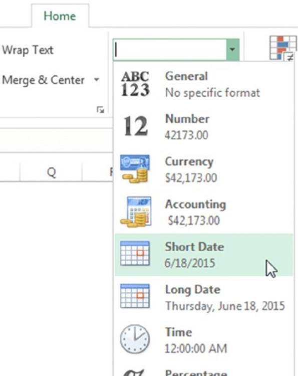
Figure 6.1 Use the Number Format drop-down list to change the appearance of dates and times.

Tip

When you create a formula that refers to a cell containing a date or a time, Excel may automatically format the formula cell as a date or a time. Sometimes, this is helpful; other times, it’s completely inappropriate and downright annoying. Unfortunately, you cannot turn off this automatic date formatting. You can, however, use a shortcut key combination to remove all number formatting from the cell and return to the default General format. Just select the cell and press Ctrl+Shift+~.

For more control over date and time formatting, select the cells and then use the Number tab of the Format Cells dialog box, as shown in Figure 6.2. Here are ways to display this dialog box:

§ Click the dialog box launcher icon of the Number group of the Home tab.

§ Click the Number Format control and choose More Number Formats from the list that appears.

§ Press Ctrl+1.

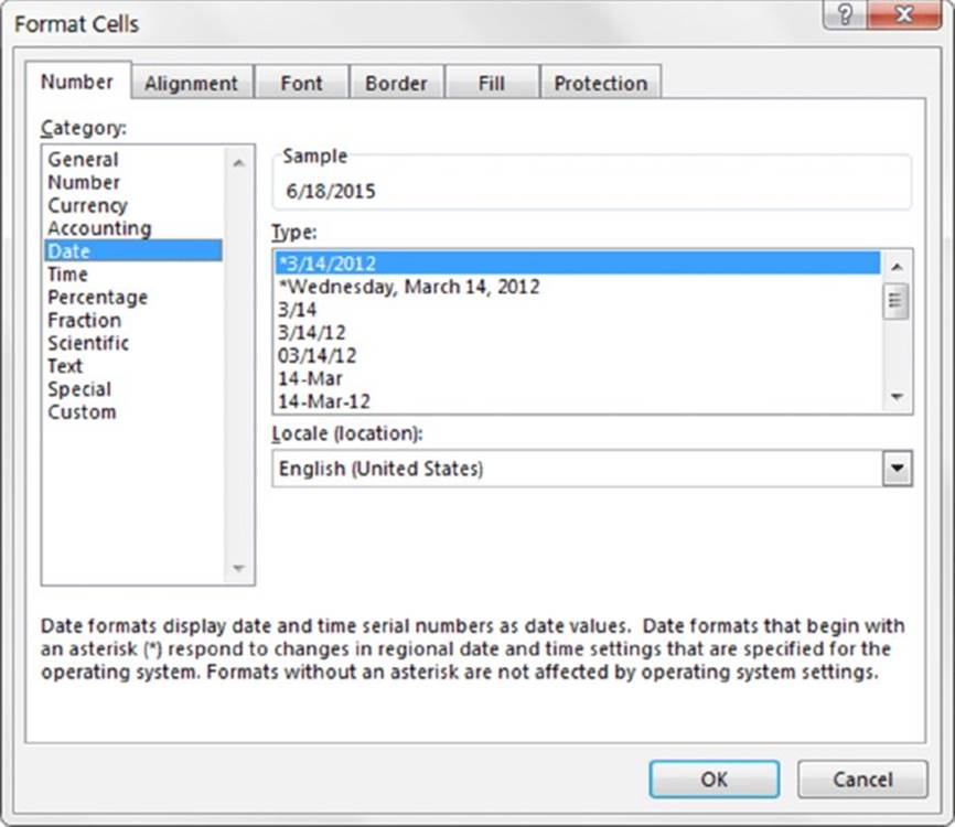
Figure 6.2 Use the Number tab of the Format Cells dialog box to change the appearance of dates and times.

The Date category shows built-in date formats, and the Time category shows built-in time formats. Additional date and time formats are available from the Custom category. Some formats include both date and time displays. Just select the desired format from the Type list and then click OK.

Note that the first two date formats in the Date category and the first time format in the Time category correspond to your Windows date and time settings.

If none of the built-in formats meets your needs, you can create a custom number format. Select the Custom category and type the custom format codes into the Type box. (See Appendix B, “Using Custom Number Formats,” for information on creating custom number formats.)

Problems with dates

Excel has some problems when it comes to dates. Many of these problems stem from the fact that Excel was designed many years ago, before the acronym Y2K became a household term. And, as we describe, the Excel designers basically emulated the Lotus 1-2-3 limited date and time features, which contain a nasty bug duplicated intentionally in Excel (described later). In addition, versions of Excel show inconsistency in how they interpret a cell entry that has a two-digit year. Finally, the way Excel interprets a date entry depends on your regional date settings.

If Excel were being designed from scratch today, I’m sure it would be much more versatile in dealing with dates. Unfortunately, we’re currently stuck with a product that leaves much to be desired in the area of dates.

The Excel leap year bug

A leap year, which occurs every four years, contains an additional day (February 29). Specifically, years that are evenly divisible by 100 are not leap years unless they are also evenly divisible by 400. Although the year 1900 was not a leap year, Excel treats it as such. In other words, when you type the following into a cell, Excel does not complain. It interprets this as a valid date and assigns a serial number of 60:

2/29/1900

If you type the following invalid date, Excel correctly interprets it as a mistake and doesn’t convert it to a date. Rather, it simply makes the cell entry a text string:

2/29/1901

How can a product used daily by millions of people contain such an obvious bug? The answer is historical. The original version of Lotus 1-2-3 contained a bug that caused it to consider 1900 as a leap year. When Excel was released some time later, the designers knew of this bug and chose to reproduce it in Excel to maintain compatibility with Lotus worksheet files.

Why does this bug still exist in later versions of Excel? Microsoft asserts that the disadvantages of correcting this bug outweigh the advantages. If the bug were eliminated, it would mess up hundreds of thousands of existing workbooks. In addition, correcting this problem would affect compatibility between Excel and other programs that use dates. As it stands, this bug really causes very few problems because most users do not use dates before March 1, 1900.

Pre-1900 dates

The world, of course, didn’t begin on January 1, 1900. People who work with historical information using Excel often need to work with dates before January 1, 1900. Unfortunately, the only way to work with pre-1900 dates is to enter the date into a cell as text. For example, you can type the following into a cell, and Excel won’t complain:

July 4, 1776

Tip

If you plan to sort information by old dates entered as text, you should enter your text dates with a four-digit year, followed by a two-digit month, and then a two-digit day, like this: 1776-07-04. This format will enable accurate sorting.

You can’t, however, perform manipulation on dates recognized as text. For example, you can’t change its numeric formatting, you can’t determine which day of the week this date occurred on, and you can’t calculate the date that occurs seven days later.

Cross-Ref

In Chapter 26, we present some custom VBA functions that enable you to work with any date in the years 0100 through 9999.

Inconsistent date entries

You need to be careful when entering dates by using two digits for the year. When you do so, Excel has some rules that kick in to determine which century to use. And those rules vary, depending on the version of Excel that you use.

Two-digit years between 00 and 29 are interpreted as 21st Century dates, and two-digit years between 30 and 99 are interpreted as 20th Century dates. For example, if you enter 12/15/28, Excel interprets your entry as December 15, 2028. However, if you enter 12/15/30, Excel sees it as December 15, 1930, because Windows uses a default boundary year of 2029. You can keep the default as is or change it by using the Windows Control Panel. Display the Regional and Language Options dialog box. Then click the Customize button to display the Customize Regional Options dialog box. Select the Date tab and then specify a different year.

Tip

The best way to avoid any surprises is to simply enter all years using all four digits for the year.

Date-Related Functions

Excel has quite a few functions that work with dates. They are all listed under the Date & Time drop-down list in the Formulas ➜ Function Library group.

Table 6.4 summarizes the date-related functions available in Excel.

Table 6.4 Date-Related Functions

* In versions prior to Excel 2007, this function is available only when the Analysis ToolPak add-in is installed.

** A function introduced in Excel 2010

*** A function introduced in Excel 2013

Displaying the current date

The following function displays the current date in a cell:

=TODAY()

You can also display the date, combined with text. The formula that follows, for example, displays text such as Today is Tuesday, April 9, 2015:

="Today is "&TEXT(TODAY(),"dddd, mmmm d, yyyy")

It’s important to understand that the TODAY function is updated whenever the worksheet is calculated. For example, if you enter either of the preceding formulas into a worksheet, the formula displays the current date. When you open the workbook tomorrow, though, it will display the current date for that day (not the date when you entered the formula).

Tip

To enter a date stamp into a cell, press Ctrl+; (semicolon). This enters the date directly into the cell and does not use a formula. Therefore, the date does not change.

Displaying any date with a function

As explained earlier in this chapter, you can easily enter a date into a cell by typing it using any of the date formats that Excel recognizes. You can also create a date by using the DATE function, which takes three arguments: the year, the month, and the day. The following formula, for example, returns a date comprising the year in cell A1, the month in cell B1, and the day in cell C1:

=DATE(A1,B1,C1)

Note

The DATE function accepts invalid arguments and adjusts the result accordingly. For example, this next formula uses 13 as the month argument and returns January 1, 2015. The month argument is automatically translated as month 1 of the following year:

=DATE(2014,13,1)

Often, you’ll use the DATE function with other functions as arguments. For example, the formula that follows uses the YEAR and TODAY functions to return the date for Independence Day (July 4th) of the current year:

=DATE(YEAR(TODAY()),7,4)

The DATEVALUE function converts a text string that looks like a date into a date serial number. The following formula returns 42238, the date serial number for August 22, 2015:

=DATEVALUE("8/22/2015")

To view the result of this formula as a date, you need to apply a date number format to the cell.

Warning

Be careful when using the DATEVALUE function. A text string that looks like a date in your country may not look like a date in another country. The preceding example works fine if your system is set for U.S. date formats, but it returns an error for other regional date formats because Excel is looking for the eighth day of the 22nd month!

Generating a series of dates

Often, you want to insert a series of dates into a worksheet. For example, in tracking weekly sales, you may want to enter a series of dates, each separated by seven days. These dates will serve to identify the sales figures.

In some cases, you can use the Excel AutoFill feature to insert a series of dates. Enter the first date and drag the cell’s fill handle while holding the right mouse button. Release the mouse button and select an option from the shortcut menu (see Figure 6.3)—Fill Days, Fill Weekdays, Fill Months, or Fill Years. Notice that Excel does not provide a Fill Weeks option.

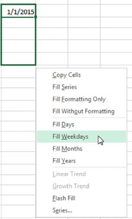
Figure 6.3 Using Excel’s AutoFill feature to create a series of dates.

For more flexibility, enter the first two dates in the series—for example, the starting day for week 1 and the starting day for week 2. Then select both cells and drag the fill handle down the column. Excel will complete the date series, with each date separated by the interval represented by the first two dates.

The advantage of using formulas (rather than the AutoFill feature) to create a series of dates is that you can change the first date, and the others will then update automatically. You need to enter the starting date into a cell and then use formulas (copied down the column) to generate the additional dates.

The following examples assume that you entered the first date of the series into cell A1 and the formula into cell A2. You can then copy this formula down the column as many times as needed.

To generate a series of dates separated by seven days, use this formula:

=A1+7

To generate a series of dates separated by one month, you need a more complicated formula because months don’t all have the same number of days. This formula creates a series of dates, separated by one month:

=DATE(YEAR(A1),MONTH(A1)+1,DAY(A1))

To generate a series of dates separated by one year, use this formula:

=DATE(YEAR(A1)+1,MONTH(A1),DAY(A1))

To generate a series of weekdays only (no Saturdays or Sundays), use the formula that follows. This formula assumes that the date in cell A1 is not a weekend day:

=IF(WEEKDAY(A1)=6,A1+3,A1+1)

Converting a nondate string to a date

You may import data that contains dates coded as text strings. For example, the following text represents August 21, 2013 (a four-digit year followed by a two-digit month, followed by a two-digit day):

20130821

To convert this string to an actual date, you can use a formula such as this one, which assumes the coded date is in cell A1:

=DATE(LEFT(A1,4),MID(A1,5,2),RIGHT(A1,2))

This formula uses text functions (LEFT, MID, and RIGHT) to extract the digits and then uses these extracted digits as arguments for the DATE function.

Cross-Ref

See Chapter 5, “Manipulating Text,” for more information about using formulas to manipulate text.

Calculating the number of days between two dates

A common type of date calculation determines the number of days between two dates. For example, you may have a financial worksheet that calculates interest earned on a deposit account. The interest earned depends on how many days the account is open. If your sheet contains the open date and the close date for the account, you can calculate the number of days the account was open.

Because dates store as consecutive serial numbers, you can use simple subtraction to calculate the number of days between two dates. For example, if cells A1 and B1 both contain a date, the following formula returns the number of days between these dates:

=A1-B1

If cell B1 contains a more recent date than the date in cell A1, the result will be negative. If you don’t care about which date is earlier and want to avoid displaying a negative value, use this formula:

=ABS(A1-B1)

Note

You can also use the DAYS worksheet function, introduced in Excel 2013. Here is an example of how to use it to calculate the number of days between two dates:

=DAYS(A1,B1)

Sometimes, calculating the difference between two days is more difficult. To demonstrate, consider the common “fence post” analogy. If somebody asks you how many units make up a fence, you can respond with either of two answers: the number of fence posts or the number of gaps between the fence posts. The number of fence posts is always one more than the number of gaps between the posts.

To bring this analogy into the realm of dates, suppose you start a sales promotion on February 1 and end the promotion on February 9. How many days was the promotion in effect? Subtracting February 1 from February 9 produces an answer of eight days. However, the promotion actually lasted nine days. In this case, the correct answer involves counting the fence posts, as it were, and not the gaps. The formula to calculate the length of the promotion (assuming you have appropriately named cells) appears like this:

=EndDay-StartDay+1

Calculating the number of work days between two dates

When calculating the difference between two dates, you may want to exclude weekends and holidays. For example, you may need to know how many business days fall in the month of November. This calculation should exclude Saturdays, Sundays, and holidays. Using the NETWORKDAYS function can help.

Note

The NETWORKDAYS function has a misleading name. This function has nothing to do with networks or networking. Rather, it calculates the net number of workdays between two dates.

The NETWORKDAYS function calculates the difference between two dates, excluding weekend days (Saturdays and Sundays). As an option, you can specify a range of cells that contain the dates of holidays, which are also excluded. Excel has absolutely no way of determining which days are holidays, so you must provide this information in a range.

Figure 6.4 shows a worksheet that calculates the workdays between two dates. The range A2:A11 contains a list of holiday dates. The formulas in column C calculate the workdays between the dates in column A and column B. For example, the formula in cell C15 is

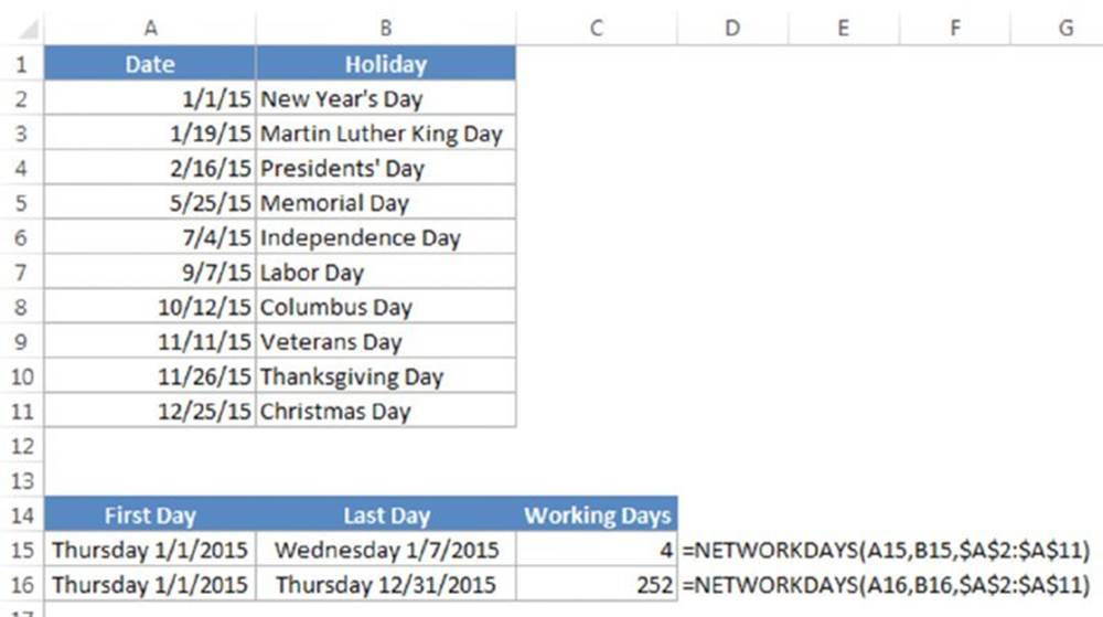
Figure 6.4 Using the NETWORKDAYS function to calculate the number of working days between two dates.

=NETWORKDAYS(A15,B15,A2:A11)

This formula returns 4, which means that the seven-day period beginning with January 1 contains four workdays. In other words, the calculation excludes one holiday, one Saturday, and one Sunday. The formula in cell C16 calculates the total number of workdays in the year.

Note

Excel 2010 introduced an updated version of the NETWORKDAYS function, named NETWORKDAYS.INTL. This version is useful if you consider weekend days to be days other than Saturday and Sunday.

On the Web

This workbook, work days.xlsx, is available at this book’s website.

Offsetting a date using only work days

The WORKDAY function is the opposite of the NETWORKDAYS function. For example, if you start a project on January 4, and the project requires 10 working days to complete, the WORKDAY function can calculate the date that you will finish the project.

The following formula uses the WORKDAY function to determine the date 10 working days from January 4, 2015. A working day is a weekday (Monday through Friday).

=WORKDAY("1/4/2015",10)

The formula returns a date serial number, which must be formatted as a date. The result is January 16, 2015. (Two weekend dates fall between January 4 and January 16.)

Warning

The preceding formula may return a different result, depending on your regional date setting. (The hard-coded date may be interpreted as April 1, 2015.) A better formula is

=WORKDAY(DATE(2015,1,4),10)

The second argument for the WORKDAY function can be negative. And, as with the NETWORKDAYS function, the WORKDAY function accepts an optional third argument (a reference to a range that contains a list of holiday dates).

Note

Excel 2010 introduced an updated version of the WORKDAY function, named WORKDAY .INTL. This version of the function is useful if you consider weekend days to be days other than Saturday and Sunday.

Calculating the number of years between two dates

The following formula calculates the number of years between two dates. This formula assumes that cells A1 and B1 both contain dates:

=YEAR(A1)-YEAR(B1)

This formula uses the YEAR function to extract the year from each date and then subtracts one year from the other. If cell B1 contains a more recent date than the date in cell A1, the result is negative.

Note that this function doesn’t calculate full years. For example, if cell A1 contains 12/31/2014, and cell B1 contains 01/01/2015, the formula returns a difference of one year even though the dates differ by only one day.

You can also use the YEARFRAC function to calculate the number of years between two dates. This function returns the number of years, including partial years. For example:

=YEARFRAC(A1,B1,1)

Because the YEARFRAC function is often used for financial applications, it uses an optional third argument that represents the “basis” for the year (for example, a 360-day year). A third argument of 1 indicates an actual year.

Calculating a person’s age

A person’s age indicates the number of full years that the person has been alive. The formula in the previous section (for calculating the number of years between two dates) won’t calculate this value correctly. You can use two other formulas, however, to calculate a person’s age.

The following formula returns the age of the person whose date of birth you enter into cell A1. This formula uses the YEARFRAC function:

=INT(YEARFRAC(TODAY(),A1,1))

The following formula uses the DATEDIF function to calculate an age. (See the sidebar “Where’s the DATEDIF function?”)

=DATEDIF(A1,TODAY(),"y")

Where’s the DATEDIF function?

In several places throughout this chapter, we refer to the DATEDIF function. You may notice that this function does not appear in the Insert Function dialog box, is not listed in the Date & Time drop-down list, and does not appear in the Formula AutoComplete list. Therefore, to use this function, you must always enter it manually.

The DATEDIF function has its origins in Lotus 1-2-3, and apparently Excel provides it for compatibility purposes. For some reason, Microsoft wants to keep this function a secret. You won’t even find the DATEDIF function in the Help files, although it’s available in all Excel versions. Strangely, DATEDIF made an appearance in the Excel 2000 Help files but hasn’t been seen since.

DATEDIF is a handy function that calculates the number of days, months, or years between two dates. The function takes three arguments: start_date, end_date, and a code that represents the time unit of interest. Here’s an example of a formula that uses the DATEDIF function. (It assumes cells A1 and A2 contain a date.) The formula returns the number of complete years between those two dates:

=DATEDIF(A1,A2,"y")

The following table displays valid codes for the third argument. You must enclose the codes in quotation marks.

The start_date argument must be earlier than the end_date argument, or the function returns an error.

Determining the day of the year

January 1 is the first day of the year, and December 31 is the last day. So, what about all those days in between? The following formula returns the day of the year for a date stored in cell A1:

=A1-DATE(YEAR(A1),1,0)

The day argument supplied is 0 (zero), calling for the “0th” day of the first month. The DATE function interprets this as the day before the first day, or December 31 of the previous year in this example. Similarly, negative numbers can be supplied for the day argument.

Here’s a similar formula that returns the day of the year for the current date:

=TODAY()-DATE(YEAR(TODAY()),1,0)

The following formula returns the number of days remaining in the year from a particular date (assumed to be in cell A1):

=DATE(YEAR(A1),12,31)-A1

When you enter this formula, Excel applies date formatting to the cell. You need to apply a nondate number format to view the result as a number.

To convert a particular day of the year (for example, the 90th day of the year) to an actual date in a specified year, use the formula that follows. This formula assumes that the year is stored in cell A1 and that the day of the year is stored in cell B1:

=DATE(A1,1,B1)

Determining the day of the week

The WEEKDAY function accepts a date argument and returns an integer between 1 and 7 that corresponds to the day of the week. The following formula, for example, returns 3 because the first day of the year 2015 falls on a Thursday:

=WEEKDAY(DATE(2015,1,1))

The WEEKDAY function uses an optional second argument that specifies the day numbering system for the result. If you specify 2 as the second argument, the function returns 1 for Monday, 2 for Tuesday, and so on. If you specify 3 as the second argument, the function returns 0 for Monday, 1 for Tuesday, and so on.

Tip

You can also determine the day of the week for a cell that contains a date by applying a custom number format. A cell that uses the following custom number format displays the day of the week, spelled out:

dddd

Determining the week of the year

To determine the week of the year for a date, use the WEEKNUM function. The following formula returns the week number for the data in cell A1:

=WEEKNUM(A1)

When you use WEEKNUM function, you can specify a second optional argument to indicate the type of week numbering system you prefer. The second argument can be one of ten values, which are described in the Help system.

Note

Excel includes the ISOWEEKNUM function. This function returns the same result as WEEKNUM with a second argument of 21.

Determining the date of the most recent Sunday

You can use the following formula to return the date for the previous Sunday. If the current day is a Sunday, the formula returns the current date. (You will need to format the cell to display as a date.)

=TODAY()-MOD(TODAY()-1,7)

To modify this formula to find the date of a day other than Sunday, change the 1 to a different number between 2 (for Monday) and 7 (for Saturday).

Determining the first day of the week after a date

This next formula returns the specified day of the week that occurs after a particular date. For example, use this formula to determine the date of the first Monday after a particular date. The formula assumes that cell A1 contains a date and that cell A2 contains a number between 1 and 7 (1 for Sunday, 2 for Monday, and so on).

=A1+A2-WEEKDAY(A1)+(A2<WEEKDAY(A1))*7

If cell A1 contains June 1, 2014 (a Sunday) and cell A2 contains 2 (for Monday), the formula returns June 2, 2014. This is the first Monday following June 1, 2014.

Determining the nth occurrence of a day of the week in a month

You may need a formula to determine the date for a particular occurrence of a weekday. For example, suppose your company payday falls on the second Friday of each month, and you need to determine the paydays for each month of the year. The following formula makes this type of calculation:

=DATE(A1,A2,1)+A3-WEEKDAY(DATE(A1,A2,1))+(A4-(A3>=WEEKDAY(DATE(A1,A2,1))))*7

The formula in this section assumes the following:

§ Cell A1 contains a year.

§ Cell A2 contains a month.

§ Cell A3 contains a day number (1 for Sunday, 2 for Monday, and so on).

§ Cell A4 contains the occurrence number (for example, 2 to select the second occurrence of the weekday specified in cell A3).

If you use this formula to determine the date of the second Tuesday in November 2015, it returns November 10, 2015.

Note

If the value in cell A4 exceeds the number of the specified day in the month, the formula returns a date from a subsequent month. For example, if you attempt to determine the date of the fifth Friday in November 2015 (there is no such date), the formula returns the first Friday in December.

Counting the occurrences of a day of the week

You can use the following formula to count the number of occurrences of a particular day of the week for a specified month. It assumes that cell A1 contains a date and that cell B1 contains a day number (1 for Sunday, 2 for Monday, and so on). The formula is an array formula, so you must enter it by pressing Ctrl+Shift+Enter.

{=SUM((WEEKDAY(DATE(YEAR(A1),MONTH(A1),ROW(INDIRECT("1:"&DAY

(DATE(YEAR(A1),MONTH(A1)+1,0))))))=B1)*1)}

If cell A1 contains the date January 6, 2015 and cell B1 contains the value 3 (for Tuesday), the formula returns 4, which reveals that January 2015 contains four Tuesdays.

The preceding array formula calculates the year and month by using the YEAR and MONTH functions. You can simplify the formula a bit if you store the year and month in separate cells. The following formula (also an array formula) assumes that the year appears in cell A1, the month in cell A2, and the day number in cell B1:

{=SUM((WEEKDAY(DATE(A1,A2,ROW(INDIRECT("1:"&DAY(DATE(A1,A2+1,0))))))=B1)*1)}

Cross-Ref

See Chapters 14, “Introducing Arrays,” and 15, “Performing Magic with Array Formulas,” for more information about array formulas.

Figure 6.5 shows this formula used in a worksheet. In this case, the formula uses mixed cell references so that you can copy it. For example, the formula in cell C3 is

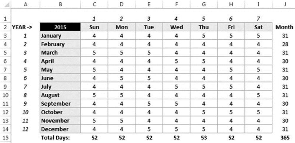
Figure 6.5 Calculating the number of each weekday in each month of a year.

{=SUM((WEEKDAY(DATE($B$2,$A3,ROW(INDIRECT("1:"&DAY(DATE($B$2,$A3+1,0))))))=C$1)*1)}

Additional formulas use the SUM function to calculate the number of days per month (column J) and the number of each weekday in the year (row 15).

On the Web

The workbook shown in Figure 6.5, day of the week count.xlsx, is available at this book’s website.

Expressing a date as an ordinal number

You may want to express the day portion of a date as an ordinal number. For example, you can display 4/16/2015 as April 16th, 2015. The following formula expresses the date in cell A1 as an ordinal date:

=TEXT(A1,"mmmm ")&DAY(A1)&IF(INT(MOD(DAY(A1),100)/10)=1, "th",IF(MOD(DAY(A1),10)=1, "st",IF(MOD(DAY(A1),10)=2,"nd",IF(MOD(DAY(A1),10)=3, "rd","th"))))&TEXT(A1,", yyyy")

Warning

The result of this formula is text, not an actual date.

The following formula shows a variation that expresses the date in cell A1 in day-month-year format. For example, 4/16/2015 would appear as 16th April, 2015. Again, the result of this formula represents text, not an actual date:

=DAY(A1)&IF(INT(MOD(DAY(A1),100)/10)=1, "th",IF(MOD(DAY(A1),10)=1, "st",

IF(MOD(DAY(A1),10)=2,"nd", IF(MOD(DAY(A1),10)=3, "rd","th"))))& " " &TEXT(A1,"mmmm, yyyy")

On the Web

This book’s website contains the workbook ordinal dates.xlsx that demonstrates the formulas for expressing dates as ordinal numbers.

Calculating dates of holidays

Determining the date for a particular holiday can be tricky. Some, such as New Year’s Day and U.S. Independence Day, are no-brainers because they always occur on the same date. For these kinds of holidays, you can simply use the DATE function, which we covered earlier in this chapter. To enter New Year’s Day (which always falls on January 1) for a specific year in cell A1, you can enter this function:

=DATE(A1,1,1)

Other holidays are defined in terms of a particular occurrence on a particular weekday in a particular month. For example, Labor Day in the United States falls on the first Monday in September.

Figure 6.6 shows a workbook with formulas to calculate the date for 11 U.S. holidays. The formulas reference the year in cell A1. Notice that because New Year’s Day, Independence Day, Veterans Day, and Christmas Day all fall on the same days each year, their dates can be calculated by using the simple DATE function.

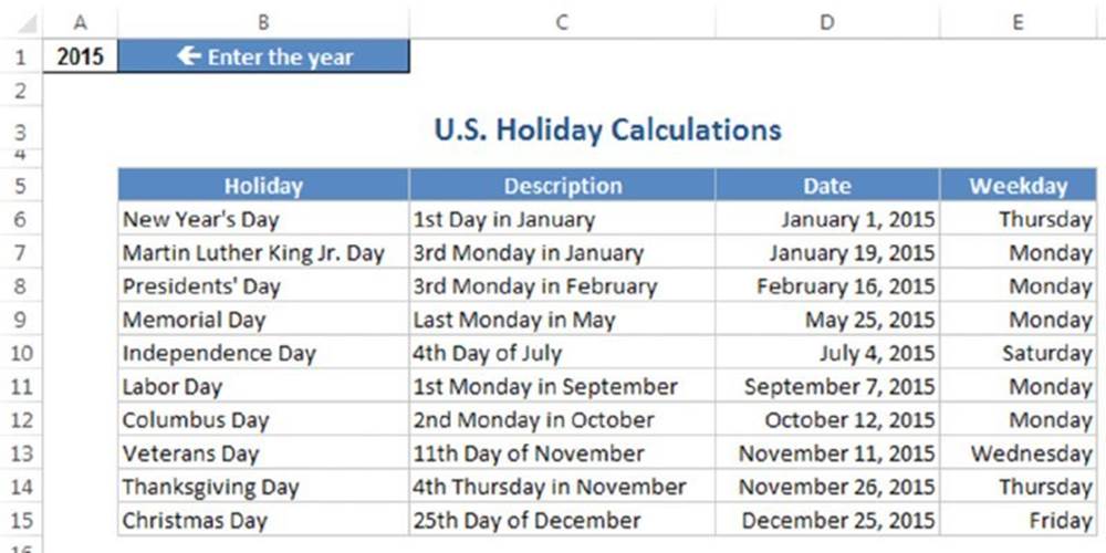
Figure 6.6 Using formulas to determine the date for various holidays.

On the Web

The workbook shown in Figure 6.6, holidays.xlsx, is available at this book’s website.

New Year’s Day

This holiday always falls on January 1:

=DATE(A1,1,1)

Martin Luther King, Jr. Day

This holiday occurs on the third Monday in January. This formula calculates Martin Luther King, Jr., Day for the year in cell A1:

=DATE(A1,1,1)+IF(2<WEEKDAY(DATE(A1,1,1)),7-WEEKDAY

(DATE(A1,1,1))+2,2-WEEKDAY(DATE(A1,1,1)))+((3-1)*7)

Presidents’ Day

Presidents’ Day occurs on the third Monday in February. This formula calculates Presidents’ Day for the year in cell A1:

=DATE(A1,2,1)+IF(2<WEEKDAY(DATE(A1,2,1)),7-WEEKDAY

(DATE(A1,2,1))+2,2-WEEKDAY(DATE(A1,2,1)))+((3-1)*7)

Easter

Calculating the date for Easter is difficult because of the complicated manner in which Easter is determined. Easter Day is the first Sunday after the next full moon occurs after the vernal equinox. These formulas were taken from the Internet and utilize a curious string of functions. We have found these formulas to be reliable, although they do not seem to work if your workbook uses the 1904 date system:

=DOLLAR(("4/"&A1)/7+MOD(19*MOD(A1,19)-7,30)*14%,)*7-6

This one is slightly shorter but equally obtuse:

=FLOOR("5/"&DAY(MINUTE(A1/38)/2+56)&"/"&A1,7)-34

Memorial Day

The last Monday in May is Memorial Day. This formula calculates Memorial Day for the year in cell A1:

=DATE(A1,6,1)+IF(2<WEEKDAY(DATE(A1,6,1)),7-WEEKDAY

(DATE(A1,6,1))+2,2-WEEKDAY(DATE(A1,6,1)))+((1-1)*7)-7

Notice that this formula actually calculates the first Monday in June and then subtracts 7 from the result to return the last Monday in May.

Independence Day

This holiday always falls on July 4:

=DATE(A1,7,4)

Labor Day

Labor Day occurs on the first Monday in September. This formula calculates Labor Day for the year in cell A1:

=DATE(A1,9,1)+IF(2<WEEKDAY(DATE(A1,9,1)),7-WEEKDAY

(DATE(A1,9,1))+2,2-WEEKDAY(DATE(A1,9,1)))+((1-1)*7)

Columbus Day

This holiday occurs on the second Monday in October. This formula calculates Columbus Day for the year in cell A1:

=DATE(A1,10,1)+IF(2<WEEKDAY(DATE(A1,10,1)),7-WEEKDAY

(DATE(A1,10,1))+2,2-WEEKDAY(DATE(A1,10,1)))+((2-1)*7)

Veterans Day

This holiday always falls on November 11:

=DATE(A1,11,11)

Thanksgiving Day

Thanksgiving Day is celebrated on the fourth Thursday in November. This formula calculates Thanksgiving Day for the year in cell A1:

=DATE(A1,11,1)+IF(5<WEEKDAY(DATE(A1,11,1)),7-WEEKDAY

(DATE(A1,11,1))+5,5-WEEKDAY(DATE(A1,11,1)))+((4-1)*7)

Christmas Day

This holiday always falls on December 25:

=DATE(A1,12,25)

Determining the last day of a month

To determine the date that corresponds to the last day of a month, you can use the DATE function. However, you need to increment the month by 1 and use a day value of 0 (zero). In other words, the 0th day of the next month is the last day of the current month.

The following formula assumes that a date is stored in cell A1. The formula returns the date that corresponds to the last day of the month:

=DATE(YEAR(A1),MONTH(A1)+1,0)

You can use a variation of this formula to determine how many days make up a specified month. The formula that follows returns an integer that corresponds to the number of days in the month for the date in cell A1.

=DAY(DATE(YEAR(A1),MONTH(A1)+1,0))

Determining whether a year is a leap year

To determine whether a particular year is a leap year, you can write a formula that determines whether the 29th day of February occurs in February or March. You can take advantage of the fact that Excel’s DATE function adjusts the result when you supply an invalid argument—for example, a day of 29 when February contains only 28 days.

The following formula returns TRUE if the year in cell A1 is a leap year; otherwise, it returns FALSE:

=IF(MONTH(DATE(A1,2,29))=2,TRUE,FALSE)

Warning

This function returns the wrong result (TRUE) if the year is 1900. See the section “The Excel leap year bug,” earlier in this chapter.

The following formula is a bit more complicated, but it correctly identifies 1900 as a nonleap year. This formula assumes that cell A1 contains a year:

=IF(OR(MOD(A1,400)=0,AND(MOD(A1,4)=0,MOD(A1,100)<>0)),TRUE, FALSE)

Determining a date’s quarter

For financial reports, you might find it useful to present information in terms of quarters. The following formula returns an integer between 1 and 4 that corresponds to the calendar quarter for the date in cell A1:

=ROUNDUP(MONTH(A1)/3,0)

This formula divides the month number by 3 and then rounds up the result.

Converting a year to roman numerals

Fans of old movies will like this one. The following formula converts the year 1945 to the Roman numerals MCMXLV:

=ROMAN(1945)

This function returns a text string, so you can’t perform calculations using the result.

Note

Use the ARABIC function to convert a Roman numeral to a value. Here’s an example, which returns 1945:

=ARABIC("MCMXLV")

Time-Related Functions

Excel includes a number of functions that enable you to work with time values in your formulas. This section contains examples that demonstrate the use of these functions.

Table 6.5 summarizes the time-related functions available in Excel. Like the date functions discussed earlier, time-related functions can be found under the Date & Time drop-down list via Formulas ➜ Function Library.

Table 6.5 Time-Related Functions

Displaying the current time

This formula displays the current time as a time serial number (or a serial number without an associated date):

=NOW()-TODAY()

You need to format the cell with a time format to view the result as a recognizable time. The quickest way is to choose Home ➜ Number ➜ Format Number and then select Time from the drop-down list.

You can also display the time, combined with text. The formula that follows displays this text: The current time is 6:28 PM.

="The current time is "&TEXT(NOW(),"h:mm AM/PM")

Note

These formulas are updated only when the worksheet is calculated. The time comes from your computer’s clock, so if the clock is wrong, the formulas will return an incorrect time.

Tip

To enter a time stamp into a cell, press Ctrl+Shift+: (colon). Excel inserts the time as a static value. (It does not change.)

Displaying any time using a function

Earlier in this chapter, we described how to enter a time value into a cell: just type it into a cell, making sure that you include at least one colon (:). You can also create a time by using the TIME function. For example, the following formula returns a time comprising the hour in cell A1, the minute in cell B1, and the second in cell C1:

=TIME(A1,B1,C1)

Like the DATE function, the TIME function accepts invalid arguments and adjusts the result accordingly. For example, the following formula uses 80 as the minute argument and returns 10:20:15 AM. The 80 minutes are simply added to the hour, with 20 minutes remaining:

=TIME(9,80,15)

Warning

If you enter a value greater than 24 as the first argument for the TIME function, the result may not be what you expect. Logically, a formula such as the one that follows should produce a date/time serial number of 1.041667 (that is, one day and one hour):

=TIME(25,0,0)

In fact, this formula is equivalent to the following:

=TIME(1,0,0)

You can also use the DATE function along with the TIME function in a single cell. The formula that follows generates a date and time with a serial number of 41612.7708333333—which represents 6:30 PM on December 4, 2013:

=DATE(2013,12,4)+TIME(18,30,0)

Note

When you enter the preceding formula, Excel formats the cell to display the date only. To see the time, you’ll need to change the number format to one that displays a date and a time.

Tip

To enter the current date and time into a cell that doesn’t change when the worksheet recalculates, press Ctrl+; (semicolon), space, Ctrl+Shift+: (colon), and then press Enter.

The TIMEVALUE function converts a text string that looks like a time into a time serial number. This formula returns 0.2395833333, which is the time serial number for 5:45 AM:

=TIMEVALUE("5:45 am")

To view the result of this formula as a time, you need to apply number formatting to the cell. The TIMEVALUE function doesn’t recognize all common time formats. For example, the following formula returns an error because Excel doesn’t like the periods in a.m.

=TIMEVALUE("5:45 a.m.")

Calculating the difference between two times

Because times are represented as serial numbers, you can subtract the earlier time from the later time to get the difference. For example, if cell A2 contains 5:30:00 and cell B2 contains 14:00:00, the following formula returns 08:30:00 (a difference of eight hours and 30 minutes):

=B2-A2

If the subtraction results in a negative value, however, it becomes an invalid time; Excel displays a series of hash marks (#######) because a time without a date has a date serial number of 0. A negative time results in a negative serial number, which cannot be displayed—although you can still use the calculated value in other formulas.

If the direction of the time difference doesn’t matter, you can use the ABS function to return the absolute value of the difference:

=ABS(B2-A2)

This “negative time” problem often occurs when calculating an elapsed time—for example, calculating the number of hours worked given a start time and an end time. This presents no problem if the two times fall in the same day. If the work shift spans midnight, though, the result is an invalid negative time. For example, you may start work at 10:00 PM and end work at 6:00 AM the next day. Figure 6.7 shows a worksheet that calculates the hours worked. As you can see, the shift that spans midnight presents a problem if you are simply subtracting the end time from the start time.

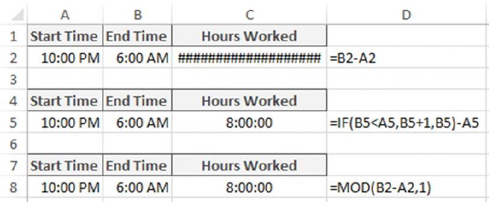
Figure 6.7 Calculating the number of hours worked returns an error if the shift spans midnight.

Using the ABS function (to calculate the absolute value) isn’t an option in this case because it will also return a wrong answer.

The following formula, however, does work:

=IF(B2<A2,B2+1,B2)-A2

Another (even simpler) formula will also do the job:

=MOD(B2-A2,1)

Tip

Negative times are permitted if the workbook uses the 1904 date system. To switch to the 1904 date system, choose Office ➜ Excel Options and then navigate to the When Calculating This Workbook section of the Advanced tab. Place a check mark next to the Use 1904 Date System option. But beware! When changing the workbook’s date system, if the workbook uses dates, the dates will be off by four years.

Summing times that exceed 24 hours

Many people are surprised to discover that when you sum a series of times that exceed 24 hours, Excel doesn’t display the correct total. Figure 6.8 shows an example. The range C1:C11 contains times that represent the hours and minutes worked each day. The formula in cell C12 follows:

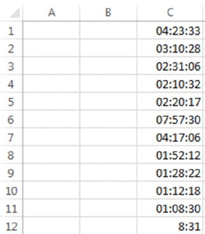
Figure 6.8 Incorrect cell formatting makes the total appear incorrectly.

=SUM(C1:C11)

As you can see, the formula returns a seemingly incorrect total (8 hours, 31 minutes). The total should read 32 hours, 31 minutes. The problem is that the formula is displaying the total as a date/time serial number of 1.35549, but the cell formatting is not displaying the date part of the date/time. The answer is incorrect because cell C12 has the wrong number format.

To view a time that exceeds 24 hours, you need to change the number format for the cell so square brackets surround the hour part of the format string. Applying the number format here to cell C12 displays the sum correctly:

[h]:mm

Figure 6.9 shows another example of a worksheet that manipulates times. This worksheet keeps track of hours worked during a week (regular hours and overtime hours).

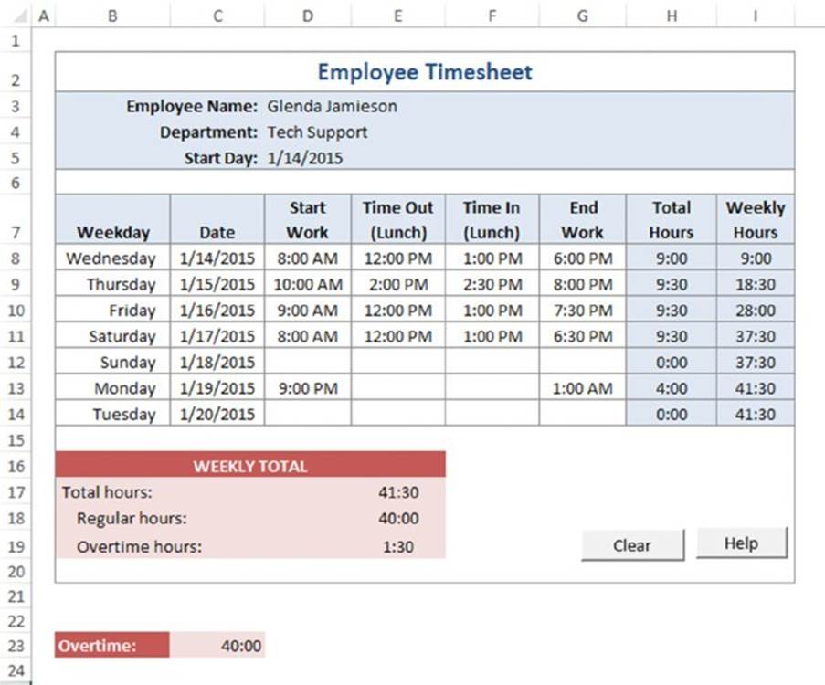
Figure 6.9 An employee timesheet workbook.

The week’s starting date appears in cell D5, and the formulas in column C fill in the dates for the days of the week. Times appear in the range D8:G14, and formulas in column H calculate the number of hours worked each day. For example, the formula in cell H8 is

=IF(E8<D8,E8+1-D8,E8-D8)+IF(G8<F8,G8+1-G8,G8-F8)

The first part of this formula subtracts the time in column D from the time in column E to get the total hours worked before lunch. The second part subtracts the time in column F from the time in column G to get the total hours worked after lunch. We use IF functions to accommodate graveyard shift cases that span midnight—for example, an employee may start work at 10:00 PM and begin lunch at 2:00 AM. Without the IF function, the formula returns a negative result.

The following formula in cell H17 calculates the weekly total by summing the daily totals in column H:

=SUM(H8:H14)

This worksheet assumes that hours that exceed 40 hours in a week are considered overtime hours. The worksheet contains a cell named Overtime (cell C23) that contains 40:00. If your standard workweek consists of something other than 40 hours, you can change the Overtime cell.

The following formula (in cell E18) calculates regular (nonovertime) hours. This formula returns the smaller of two values: the total hours, or the overtime hours:

=MIN(E17,Overtime)

The final formula, in cell E19, simply subtracts the regular hours from the total hours to yield the overtime hours:

=E17-E18

The times in H17:H19 may display time values that exceed 24 hours, so these cells use a custom number format:

[h]:mm

On the Web

The workbook shown in Figure 6.9, time sheet.xlsm, is available at this book’s website.

Converting from military time

Military time is expressed as a four-digit number from 0000 to 2359. For example, 1:00 AM is expressed as 0100 hours, and 3:30 PM is expressed as 1530 hours. The following formula converts such a number (assumed to appear in cell A1) to a standard time:

=TIMEVALUE(LEFT(A1,2)&":"&RIGHT(A1,2))

The formula returns an incorrect result if the contents of cell A1 do not contain four digits. The following formula corrects the problem and returns a valid time for any military time value from 0 to 2359:

=TIMEVALUE(LEFT(TEXT(A1,"0000"),2)&":"&RIGHT(A1,2))

The following is a simpler formula that uses the TEXT function to return a formatted string and then uses the TIMEVALUE function to express the result in terms of a time:

=TIMEVALUE(TEXT(A1,"00\:00"))

Converting decimal hours, minutes, or seconds to a time

To convert decimal hours to a time, divide the decimal hours by 24. For example, if cell A1 contains 9.25 (representing hours), this formula returns 09:15:00 (9 hours, 15 minutes):

=A1/24

To convert decimal minutes to a time, divide the decimal minutes by 1,440 (the number of minutes in a day). For example, if cell A1 contains 500 (representing minutes), the following formula returns 08:20:00 (8 hours, 20 minutes):

=A1/1440

To convert decimal seconds to a time, divide the decimal seconds by 86,400 (the number of seconds in a day). For example, if cell A1 contains 65,000 (representing seconds), the following formula returns 18:03:20 (18 hours, 3 minutes, and 20 seconds):

=A1/86400

Adding hours, minutes, or seconds to a time

You can use the TIME function to add any number of hours, minutes, or seconds to a time. For example, assume that cell A1 contains a time. The following formula adds two hours and 30 minutes to that time and displays the result:

=A1+TIME(2,30,0)

You can use the TIME function to fill a range of cells with incremental times. Figure 6.10 shows a worksheet with a series of times in ten-minute increments. Cell A1 contains a time that was entered directly. Cell A2 contains the following formula, which was copied down the column:

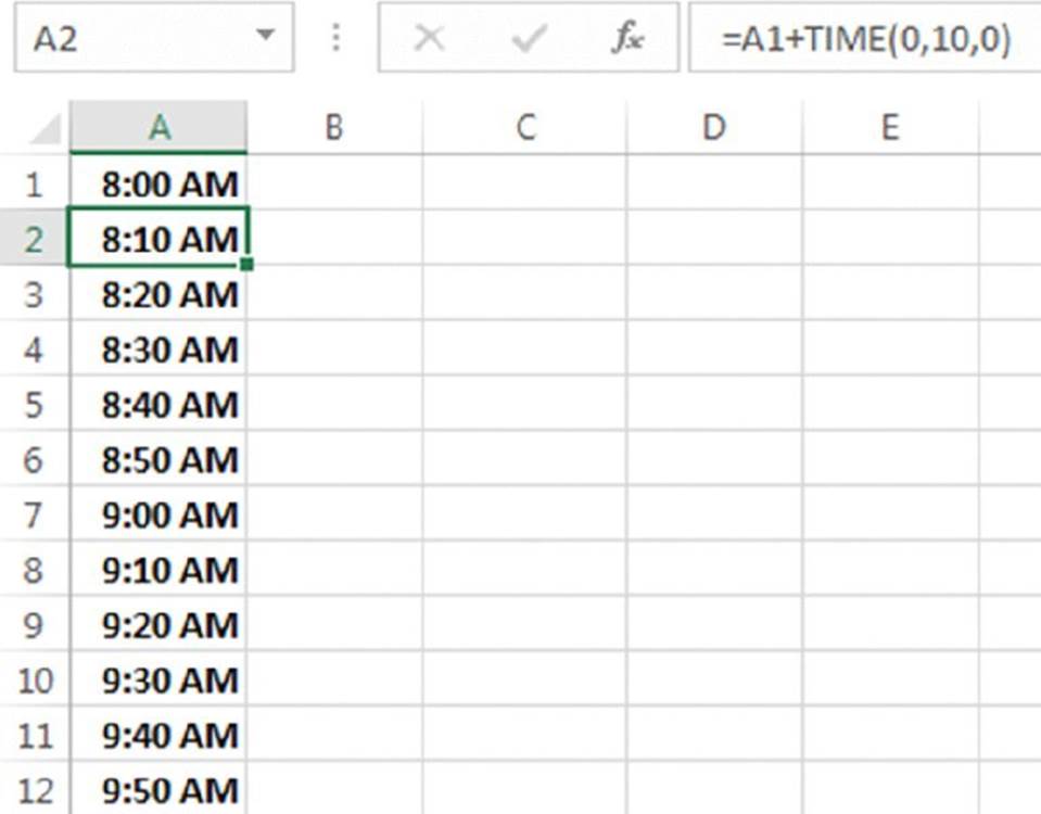
Figure 6.10 Using a formula to create a series of incremental times.

=A1+TIME(0,10,0)

Tip

You can also use the Excel AutoFill feature to fill a range with times. For example, to create a series of times with 10-minute increments, type 8:00 AM in cell A1 and 8:10 AM in cell A2. Select both cells and then drag the fill handle (in the lower-right corner of cell A2) down the column to create the series.

Converting between time zones

You may receive a worksheet that contains dates and times in Greenwich Mean Time (GMT, sometimes referred to as Zulu time), and you may need to convert these values to local time. To convert dates and times into local times, you need to determine the difference in hours between the two time zones. For example, to convert GMT times to U.S. Central Standard Time (CST), the hour conversion factor is –6.

You can’t use the TIME function with a negative argument, so you need to take a different approach. One hour equals 1/24 of a day, so you can divide the time conversion factor by 24 and then add it to the time.

Figure 6.11 shows a worksheet set up to convert dates and times (expressed in GMT) to local times. Cell B1 contains the hour conversion factor (–5 hours for U.S. Eastern Standard Time; EST). The formula in B4, which copies down the column, is this:

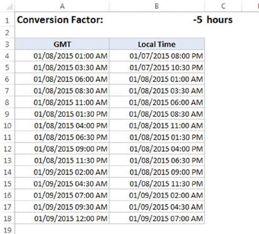
Figure 6.11 This worksheet converts dates and times between time zones.

=A4+($B$1/24)

On the Web

You can download the workbook shown in Figure 6.11, gmt conversion.xlsx, from this book’s website.

This formula effectively adds x hours to the date and time in column A. If cell B1 contains a negative hour value, the value subtracts from the date and time in column A. Note that, in some cases, this also affects the date.

Rounding time values

You may need to create a formula that rounds a time to a particular value. For example, you may need to enter your company’s time records rounded to the nearest 15 minutes. This section presents examples of various ways to round a time value.

The following formula rounds the time in cell A1 to the nearest minute:

=ROUND(A1*1440,0)/1440

The formula works by multiplying the time by 1440 (to get total minutes). This value is passed to the ROUND function, and the result is divided by 1440. For example, if cell A1 contains 11:52:34, the formula returns 11:53:00.

The following formula resembles this example, except that it rounds the time in cell A1 to the nearest hour:

=ROUND(A1*24,0)/24

If cell A1 contains 5:21:31, the formula returns 5:00:00.

The following formula rounds the time in cell A1 to the nearest 15 minutes (quarter of an hour):

=ROUND(A1*24/0.25,0)*(0.25/24)

In this formula, 0.25 represents the fractional hour. To round a time to the nearest 30 minutes, change 0.25 to 0.5, as in the following formula:

=ROUND(A1*24/0.5,0)*(0.5/24)

Calculating Durations

Sometimes, you may want to work with time values that don’t represent an actual time of day. For example, you might want to create a list of the finish times for a race or record the time you spend jogging each day. Such times don’t represent a time of day. Rather, a value represents the time for an event (in hours, minutes, and seconds). The time to complete a test, for instance, might be 35 minutes and 45 seconds. You can enter that value into a cell as follows:

00:35:45

Excel interprets such an entry as 12:35:45 AM, which works fine (just make sure that you format the cell so it appears as you like). When you enter such times that do not have an hour component, you must include at least one zero for the hour. If you omit a leading zero for a missing hour, Excel interprets your entry as 35 hours and 45 minutes.

Figure 6.12 shows an example of a worksheet set up to keep track of someone’s jogging activity. Column A contains simple dates. Column B contains the distance, in miles. Column C contains the time it took to run the distance. Column D contains formulas to calculate the speed, in miles per hour. For example, the formula in cell D2 is this:

=B2/(C2*24)

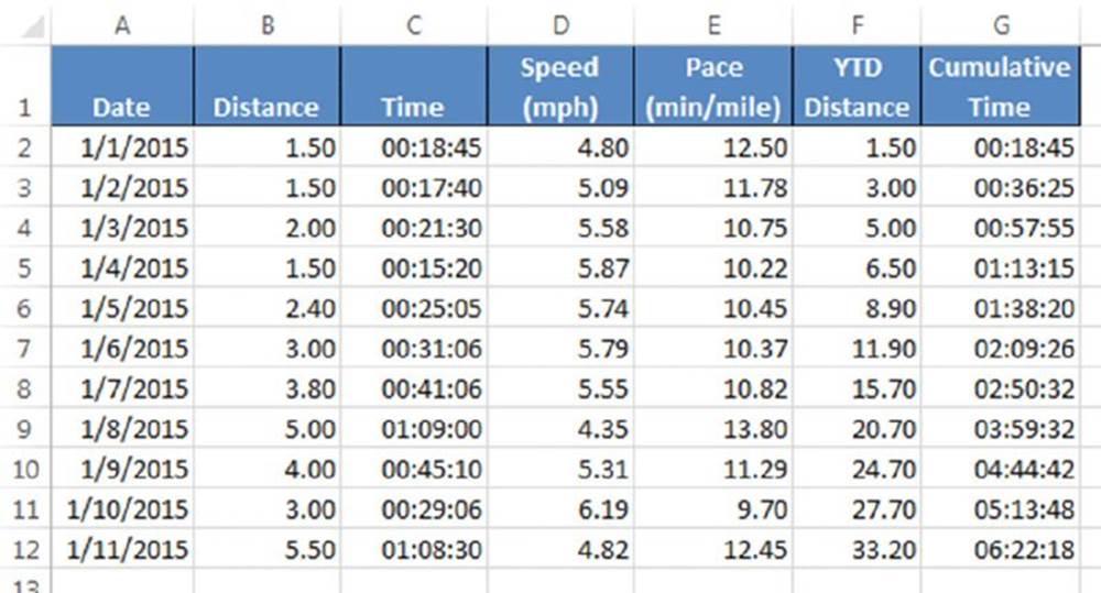
Figure 6.12 This worksheet uses times not associated with a time of day.

Column E contains formulas to calculate the pace, in minutes per mile. For example, the formula in cell E2 is this:

=(C2*60*24)/B2

Columns F and G contain formulas that calculate the year-to-date distance (using column B) and the cumulative time (using column C). The cells in column G are formatted using the following number format (which permits time displays that exceed 24 hours):

[hh]:mm:ss

On the Web

You can access the workbook shown in Figure 6.12, jogging log.xlsx, at this book’s website.