Excel 2016 Formulas (2016)

PART II
Leveraging Excel Functions

Chapter 5
Manipulating Text

In This Chapter

· How Excel handles text entered into cells

· Excel worksheet functions that handle text

· Examples of advanced text formulas

Excel, of course, is best known for its ability to crunch numbers. However, it is also quite versatile when it comes to handling text. As you know, Excel enables you to enter text for items such as row and column headings, customer names and addresses, part numbers, and just about anything else. And, as you might expect, you can use formulas to manipulate the text contained in cells.

This chapter contains many examples of formulas that use functions to manipulate text. Some of these formulas perform feats that you may not have thought possible.

A Few Words About Text

When you type data into a cell, Excel immediately goes to work and determines whether you’re entering a formula, a number (including a date or time), or anything else. Anything else is considered text.

Note

You may hear the term string used instead of text. You can use these terms interchangeably. Sometimes they even appear together, as in text string.

How many characters in a cell?

A single cell can hold up to 32,000 characters. To put things into perspective, this chapter contains about 30,000 characters. We certainly don’t recommend using a cell in lieu of a word processor, but you really don’t have to lose much sleep worrying about filling up a cell with text.

Numbers as text

As we mentioned, Excel distinguishes between numbers and text. In some cases, such as part numbers and credit card numbers, you don’t need a number to be numerical. If you want to “force” a number to be considered as text, you can do one of the following:

§ Apply the Text number format to the cell before you enter the number. Select Text from the Number Format drop-down list, which can be found in the Home ➜ Number group. If you haven’t applied other horizontal alignment formatting, the value will appear left aligned in the cell (like normal text), and functions like SUM will not treat it as a value. Note, however, that it doesn’t work in the opposite direction. If you enter a number and then format it as text, the number will be left aligned, but functions will continue to treat the entry as a value.

§ Precede the number with an apostrophe. The apostrophe isn’t displayed, but the cell entry will be treated as if it were text. Functions like SUM will not treat the cell as a number.

Even though a cell is formatted as text (or uses an apostrophe), you can still perform some mathematical operations on the cell if the entry looks like a number. For example, assume cell A1 contains a numeric value preceded by an apostrophe. This formula displays the value in A1, incremented by 1:

=A1+1

This formula, however, treats the contents of cell A1 as 0:

=SUM(A1:A10)

To confuse things even more, if you format cell A1 as text, the preceding SUM formula treats it as 0.

In some cases, treating text as a number can be useful. In other cases, it can cause problems. Bottom line? Just be aware of Excel’s inconsistency in how it treats a number formatted as text.

Note

If background error checking is turned on, Excel flags numbers preceded by an apostrophe (and numbers in cells formatted as text before the number was entered) with a small triangle indicator in the cell’s upper-left corner. Activate a cell that displays such an indicator, and Excel displays an icon. Click the icon, and you have several options on how to handle that potential error. Figure 5.1 shows an example. Background error checking is controlled from the Excel Options dialog box. Choose File ➜ Options and navigate to the Error Checking section of the Formulas tab.

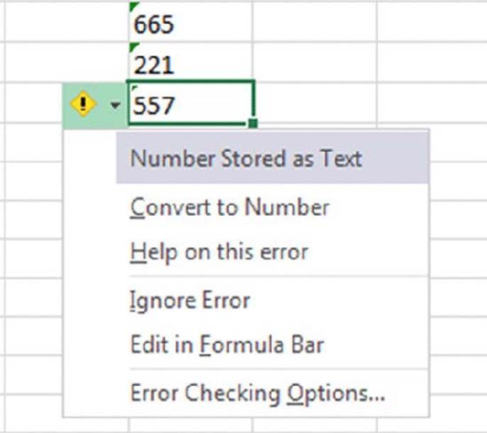
Figure 5.1 Excel’s background error checking flags numbers that are formatted as text.

When a number isn’t treated as a number

If you import data into Excel, you may be aware of a common problem: sometimes the imported values are treated as text. Here’s a quick way to convert these nonnumbers to actual values. Activate any empty cell and choose Home ➜ Clipboard ➜ Copy. Then select the range that contains the values you need to fix. Choose Home ➜Clipboard ➜ Paste ➜ Paste Special. In the Paste Special dialog box, select the Add option, and then click OK. By “adding zero” to the text, you force Excel to treat the nonnumbers as actual values.

If background error checking is enabled, Excel will usually identity such nonnumber cells and give you an opportunity to convert them.

Text Functions

Excel has an excellent assortment of worksheet functions that can handle text. For your convenience, the Function Library group on the Formulas tab includes a Text drop-down list that provides access to most of these functions. A few other functions that are relevant to text manipulation appear in other function categories. For example, the ISTEXT function is in the Information category (Formulas ➜ Function Library ➜ More Functions ➜ Information).

Cross-Ref

Refer to Appendix A, “Excel Function Reference,” for a complete list of the functions in the Text category.

Most of the functions in the Text category are not limited for use with text. In other words, these functions can also operate with cells that contain values. Excel is very accommodating when it comes to treating numbers as text and text as numbers.

The examples in this section demonstrate some common (and useful) things that you can do with text. You may need to adapt some of these examples for your own use.

Determining whether a cell contains text

In some situations, you may need a formula that determines the type of data contained in a particular cell. For example, you can use an IF function to return a result only if a cell contains text. The easiest way to make this determination is to use the ISTEXT function.

The ISTEXT function takes a single argument, returning TRUE if the argument contains text and FALSE if it doesn’t contain text. The formula that follows returns TRUE if A1 contains a string:

=ISTEXT(A1)

You can also use the TYPE function. The TYPE function takes a single argument and returns a value that indicates the type of data in a cell. If cell A1 contains a text string, the formula that follows returns 2 (the code number for text):

=TYPE(A1)

Both the ISTEXT function and the TYPE function consider a numeric value that’s preceded by an apostrophe to be text. However, these functions do not consider a number formatted as Text to be text unless the Text formatting is applied before you enter the number in the cell.

This sounds very confusing (and it is), but in actual practice, it’s rare to need to identify the contents of a cell as numeric or text.

Working with character codes

Every character that you see on your screen has an associated code number. For Windows systems, Excel uses the standard American National Standards Institute (ANSI) character set. The ANSI character set consists of 255 characters, numbered from 1 to 255. An ANSI character requires one byte of storage. Excel also supports an extended character set known as Unicode, in which each character requires two bytes of storage.

Figure 5.2 shows an Excel worksheet that displays all 255 ANSI characters. This example uses the Calibri font. (Other fonts may have different characters.)

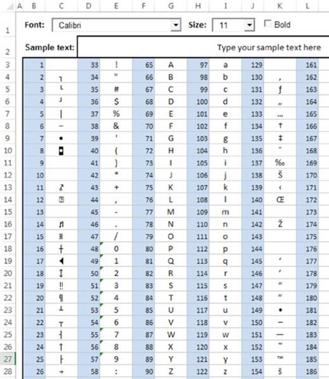
Figure 5.2 The ANSI character set (for the Calibri font).

On the Web

This book’s website includes a copy of the workbook character set.xlsm. It has some simple macros that enable you to display the character set for any font installed on your system.

Two functions come into play when dealing with character codes: CODE and CHAR. These functions aren’t very useful by themselves. However, they can prove quite useful in conjunction with other functions. We discuss these functions in the following sections.

Note

The CODE and CHAR functions work only with ANSI strings. Excel 2013 introduced two functions that are similar to CODE and CHAR but work with double-byte Unicode characters. These functions are UNICODE and UNICHAR.

The CODE function

Excel’s CODE function returns the ANSI character code for its argument. The formula that follows returns 65, the character code for uppercase A:

=CODE("A")

If the argument for CODE consists of more than one character, the function uses only the first character. Therefore, this formula also returns 65:

=CODE("Abbey Road")

The CHAR function

The CHAR function is essentially the opposite of the CODE function. Its argument is a value between 1 and 255; the function returns the corresponding character. The following formula, for example, returns the letter A:

=CHAR(65)

To demonstrate the opposing nature of the CODE and CHAR functions, try entering this formula:

=CHAR(CODE("A"))

This formula (illustrative rather than useful) returns the letter A. First it converts the character to its code value (65), and then it converts this code back to the corresponding character.

Assume that cell A1 contains the letter A (uppercase). The following formula returns the letter a (lowercase):

=CHAR(CODE(A1)+32)

This formula takes advantage of the facts that the alphabetic characters in most fonts appear in alphabetical order within the character set, and the lowercase letters follow the uppercase letters (with a few other characters tossed in between). Each lowercase letter lies exactly 32 character positions higher than its corresponding uppercase letter.

How to find special characters

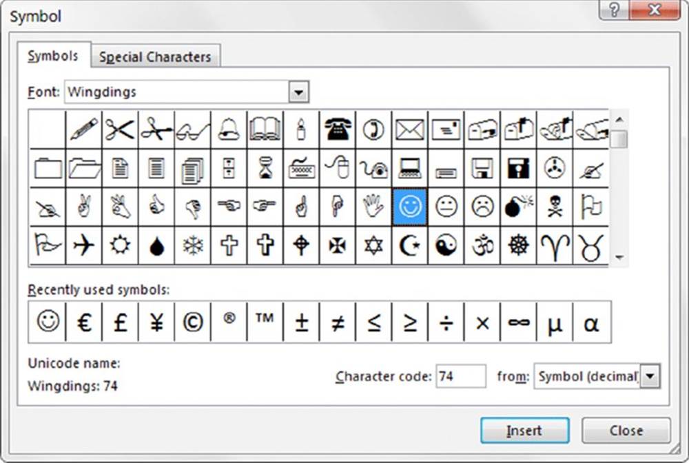
Don’t overlook the handy Symbol dialog box (which appears when you choose Insert ➜ Symbols ➜ Symbol). This dialog box makes it easy to insert special characters (including Unicode characters) into cells. For example, you might (for some strange reason) want to include a smiley face character in your spreadsheet. From the Symbol dialog box, select the Wingdings font (see the accompanying figure). Examine the characters, locate the smiley face, click Insert, and then click Cancel. You’ll also find out that this character has a code of 74.

In addition, Excel has several built-in AutoCorrect symbols. For example, if you type (c) followed by a space or the Enter key, Excel converts the (c) to a copyright symbol.

To see the other symbols that you can enter this way, display the AutoCorrect dialog box by choosing File ➜ Options. On the Proofing tab in the Excel Options dialog box, click the AutoCorrect Options button. You can then scroll through the list to see which autocorrections are enabled (and delete those that you don’t want).

If you find that Excel makes an autocorrection that you don’t want, press Ctrl+Z immediately to undo it.

Determining whether two strings are identical

You can enter a simple logical formula to determine whether two cells contain the same entry. For example, use this formula to determine whether cell A1 has the same contents as cell A2:

=A1=A2

Excel acts a bit lax in its comparisons when text is involved. Consider the case in which A1 contains the word January (initial capitalization), and A2 contains JANUARY (all uppercase). You’ll find that the previous formula returns TRUE even though the contents of the two cells are not really the same. In other words, the comparison is not case sensitive.

In many cases, you don’t need to worry about the case of the text. However, if you need to make an exact, case-sensitive comparison, you can use Excel’s EXACT function. The formula that follows returns TRUE only if cells A1 and A2 contain exactly the same entry:

=EXACT(A1,A2)

The following formula returns FALSE because the two strings do not match exactly with respect to case:

=EXACT("California","california")

Joining two or more cells

Excel uses an ampersand (&) as its concatenation operator. Concatenation is simply a fancy term that describes what happens when you join the contents of two or more cells. For example, if cell A1 contains the text Tucson, and cell A2 contains the text Arizona, the following formula then returns TucsonArizona:

=A1&A2

Notice that the two strings are joined without an intervening space. To add a space between the two entries (to get Tucson Arizona), use a formula like this one:

=A1&" "&A2

Or, even better, use a comma and a space to produce Tucson, Arizona:

=A1&", "&A2

Another option is to eliminate the quote characters and use the CHAR function with an appropriate argument. Note this example of using the CHAR function to represent a comma (44) and a space (32):

=A1&CHAR(44)&CHAR(32)&A2

If you’d like to force a line break between strings, concatenate the strings by using CHAR(10), which inserts a line break character. Also, make sure that you apply the wrap text format to the cell. (Choose Home ➜ Alignment ➜ Wrap Text.) The following example joins the text in cell A1 and the text in cell B1 with a line break in between:

=A1&CHAR(10)&B1

The following formula returns the string Stop by concatenating four characters returned by the CHAR function:

=CHAR(83)&CHAR(116)&CHAR(111)&CHAR(112)

Here’s a final example of using the & operator. In this case, the formula combines text with the result of an expression that returns the maximum value in column C:

="The largest value in Column C is " &MAX(C:C)

Note

Excel also has a CONCATENATE function, which takes up to 255 arguments. This function simply combines the arguments into a single string. You can use this function if you like, but using the & operator is usually simpler and results in shorter formulas.

Cross-Ref

In some cases, the Flash Fill feature can substitute for creating formulas that concatenate text. See Chapter 16, “Importing and Cleaning Data,” for more information.

Displaying formatted values as text

The Excel TEXT function enables you to display a value in a specific number format. Although this function may appear to have dubious value, it does serve some useful purposes, as the examples in this section demonstrate. Figure 5.3 shows a simple worksheet. The formula in cell D2 is

="The net profit is " & B2

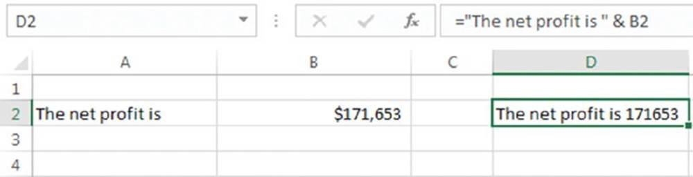
Figure 5.3 The formula in cell D2 doesn’t display the formatted number.

This formula essentially combines a text string with the contents of cell B2 and displays the result. Note, however, that the value from cell B2 is not formatted in any way. You might want to display the contents in cell B2 using a currency number format.

Note

Contrary to what you might expect, applying a number format to the cell that contains the formula has no effect. This is because the formula returns a string, not a value.

We can use the TEXT function to simulate the number formatting shown in cell D2:

="The net profit is " & TEXT(B2,"$#,##0.00")

This formula displays the text along with a nicely formatted value: The net profit is $171,653.

The second argument for the TEXT function consists of a standard Excel number format string. You can enter any valid number format string for this argument. Note, however, that color codes in number format strings are ignored.

The preceding example uses a simple cell reference (B2). You can, of course, use an expression instead. Here’s an example that combines text with a number resulting from a computation:

="Average Expenditure: "& TEXT(AVERAGE(A:A),"$#,##0.00")

This formula might return a string such as Average Expenditure: $7,794.57.

Here’s another example that uses the NOW function (which returns the current date and time). The TEXT function displays the date and time, nicely formatted:

="Report printed on "&TEXT(NOW(),"mmmm d, yyyy, at h:mm AM/PM")

Cross-Ref

In Chapter 6, “Working with Dates and Times,” we discuss how Excel handles dates and times.

The formula might display the following: Report printed on July 22, 2015 at 3:23 PM.

Cross-Ref

Refer to Appendix B, “Using Custom Number Formats,” for details on Excel number formats.

Displaying formatted currency values as text

Excel’s DOLLAR function converts a number to text using the currency format. It takes two arguments: the number to convert, and the number of decimal places to display. The DOLLAR function uses the regional currency symbol (for example, $).

You can sometimes use the DOLLAR function in place of the TEXT function. The TEXT function, however, is much more flexible because it doesn’t limit you to a specific number format. The second argument for the DOLLAR function specifies the number of decimal places.

The following formula returns Total: $1,287.37:

="Total: " & DOLLAR(1287.367, 2)

Note

If you’re looking for a function that converts a number into spelled-out text (such as One hundred twelve and 32/100 dollars), you won’t find such a function. Well, Excel does have a function—BAHTTEXT—but it converts the number into the Thai language. Why Excel doesn’t include an English language version of this function remains a mystery. VBA can often be used to overcome Excel’s deficiencies, though. In Chapter 26, “VBA Custom Function Examples,” you’ll find a custom VBA worksheet function called SPELLDOLLARS, which displays dollar amounts as English text.

Removing excess spaces and nonprinting characters

Often, data imported into an Excel worksheet contains excess spaces or strange (often unprintable) characters. Excel provides you with two functions to help whip your data into shape: TRIM and CLEAN:

§ TRIM removes all leading and trailing spaces, and it replaces internal strings of multiple spaces with a single space.

§ CLEAN removes all nonprinting characters from a string. These “garbage” characters often appear when you import certain types of data.

This example uses the TRIM function. The formula returns Fourth Quarter Earnings (with no excess spaces):

=TRIM(" Fourth Quarter Earnings ")

Cross-Ref

See Chapter 16 for detailed coverage of cleaning up data.

Counting characters in a string

The LEN function takes one argument and returns the number of characters in the argument. For example, assume that cell A1 contains the string September Sales. The following formula returns 15:

=LEN(A1)

Notice that space characters are included in the character count. The LEN function can be useful for identifying strings with extraneous spaces, which can cause problems in some situations, such as in lookup formulas. The following formula returns FALSE if cell A1 contains any leading spaces, trailing spaces, or multiple spaces.

=LEN(A1)=LEN(TRIM(A1))

The following formula shortens text that is too long. If the text in A1 is more than ten characters in length, this formula returns the first nine characters plus an ellipsis (133 on the ANSI chart) as a continuation character. If cell A1 contains ten or fewer characters, the entire string is returned:

=IF(LEN(A1)>10,LEFT(A1,9)&CHAR(133),A1)

Cross-Ref

Later in this chapter, you’ll see sample formulas that demonstrate how to count the number of a specific character within a string. (See the “Advanced Text Formulas” section.) Also, Chapter 7, “Counting and Summing Techniques,” contains additional counting techniques. Still more counting examples are provided in Chapter 15, “Performing Magic with Array Formulas,” which deals with array formulas.

Repeating a character or string

The REPT function repeats a text string (first argument) any number of times you specify (second argument). For example, this formula returns HoHoHo:

=REPT("Ho",3)

You can also use this function to create a crude horizontal divider between cells. This example displays a squiggly line, 20 characters in length:

=REPT("~",20)

Creating a text histogram

A clever use for the REPT function is to create a simple histogram (also known as a frequency distribution) directly in a worksheet (chart not required). Figure 5.4 shows an example of such a histogram. You’ll find this type of graphical display especially useful when you need to visually summarize many values. In such a case, a standard chart may be unwieldy.

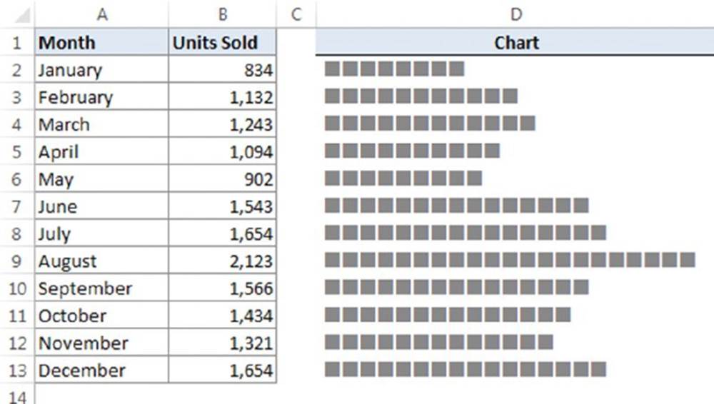
Figure 5.4 Using the REPT function to create a histogram in a worksheet range.

Tip

The data bars conditional formatting feature is a much better way to display a simple histogram directly in cells. See Chapter 19, “Conditional Formatting,” for more information about data bars.

The formulas in column D graphically depict the values in column B by displaying a series of characters in the Wingdings 2 font. This example uses character code 162, which displays as a solid rectangle in the Wingdings 2 font. A formula using the REPT function determines the number of characters displayed. Cell D2 contains this formula:

=REPT(CHAR(162),B2/100)

Assign the Wingdings 2 font to cell D2 and then copy the formulas down the column to accommodate all the data. Depending on the numerical range of your data, you may need to change the scaling. Experiment by replacing the 100 value in the formulas. You can substitute any character you like to produce a different character in the chart.

On the Web

The workbook shown in Figure 5.4, text histogram.xlsx, is available at this book’s website and contains another example of this technique.

Padding a number

You’re probably familiar with a common security measure (frequently used on printed checks) in which numbers are padded with asterisks on the right. The following formula displays the value in cell A1, along with enough asterisks to make 24 characters total:

=(A1 & REPT("*",24-LEN(A1)))

Or if you’d prefer to pad the number with asterisks on the left, use this formula:

=REPT("*",24-LEN(A1))&A1

The following formula displays asterisk padding on both sides of the number. It returns 24 characters when the number in cell A1 contains an even number of characters; otherwise, it returns 23 characters:

=REPT("*",12-LEN(A1)/2)&A1&REPT("*",12-LEN(A1)/2)

The preceding formulas are a bit deficient because they don’t show any number formatting. Note this revised version that displays the value in A1 (formatted), along with the asterisk padding on the left:

=REPT("*",24-LEN(TEXT(A1,"$#,##0.00")))&TEXT(A1,"$#,##0.00")

Figure 5.5 shows these formulas in action.

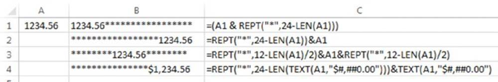
Figure 5.5 Using a formula to pad a number with asterisks.

You can also pad a number by using a custom number format. To repeat the next character in the format to fill the column width, include an asterisk (*) in the custom number format code. For example, use this number format to pad the number with dashes:

$#,##0.00*-

To pad the number with asterisks, use two asterisks, like this:

$#,##0.00**

Cross-Ref

See Appendix B for more information about custom number formats, including additional examples using the asterisk format code.

Changing the case of text

Excel provides three handy functions to change the case of text:

§ UPPER: Converts the text to ALL UPPERCASE.

§ LOWER: Converts the text to all lowercase.

§ PROPER: Converts the text to Proper Case. (The First Letter In Each Word Is Capitalized.)

These functions are quite straightforward. The formula that follows, for example, converts the text in cell A1 to proper case. If cell A1 contained the text MR. JOHN Q. PUBLIC, the formula would return Mr. John Q. Public:

=PROPER(A1)

These functions operate only on alphabetic characters; they ignore all other characters and return them unchanged.

Caution

The PROPER function capitalizes the first letter of every word, which isn’t always desirable. Applying the PROPER function to a tale of two cities results in A Tale Of Two Cities. Normally, the preposition of wouldn’t be capitalized. In addition, applying the PROPER function to a name such as ED MCMAHON results in Ed Mcmahon (not Ed McMahon). And, apparently, the function is programmed to capitalize the letter following an apostrophe. Using the function with an argument of don’t results inDon’T. But if the argument is o’reilly, it works perfectly.

Transforming data with formulas

Many of the examples in this chapter describe how to use functions to transform data in some way. For example, you can use the UPPER function to transform text into uppercase. Often, you’ll want to replace the original data with the transformed data. To do so, paste values over the original text. Here’s how:

1. Create your formulas to transform the original data.

2. Select the formula cells.

3. Choose Home ➜ Clipboard ➜ Copy (or press Ctrl+C).

4. Select the original data cells.

5. Choose Home ➜ Clipboard ➜ Paste ➜ Values (V).

After performing these steps, you can delete the formulas.

Extracting characters from a string

Excel users often need to extract characters from a string. For example, you may have a list of employee names (first and last names) and need to extract the last name from each cell. Excel provides several useful functions for extracting characters:

§ LEFT: Returns a specified number of characters from the beginning of a string

§ RIGHT: Returns a specified number of characters from the end of a string

§ MID: Returns a specified number of characters beginning at any specified position within a string

The formula that follows returns the last 10 characters from cell A1. If A1 contains fewer than 10 characters, the formula returns all the text in the cell:

=RIGHT(A1,10)

This next formula uses the MID function to return five characters from cell A1, beginning at character position 2. In other words, it returns characters 2 through 6:

=MID(A1,2,5)

The following example returns the text in cell A1, with only the first letter in uppercase (sometimes referred to as sentence case). It uses the LEFT function to extract the first character and convert it to uppercase. This character then concatenates to another string that uses the RIGHT function to extract all but the first character (converted to lowercase):

=UPPER(LEFT(A1))&LOWER(RIGHT(A1,LEN(A1)-1))

If cell A1 contained the text FIRST QUARTER, the formula would return First quarter.

Replacing text with other text

In some situations, you may need a formula to replace a part of a text string with some other text. For example, you may import data that contains asterisks, and you may need to convert the asterisks to some other character. You could use Excel’s Home ➜ Editing ➜ Find & Select ➜ Replace command to make the replacement. If you prefer a formula-based solution, you can take advantage of either of two functions:

§ SUBSTITUTE replaces specific text in a string. Use this function when you know the character(s) that you want to replace but not the position.

§ REPLACE replaces text that occurs in a specific location within a string. Use this function when you know the position of the text that you want to replace but not the actual text.

The following formula uses the SUBSTITUTE function to replace 2012 with 2013 in the string 2012 Budget. The formula returns 2013 Budget:

=SUBSTITUTE("2012 Budget","2012","2013")

The following formula uses the SUBSTITUTE function to remove all spaces from a string. In other words, it replaces all space characters with an empty string. The formula returns 2013OperatingBudget:

=SUBSTITUTE("2013 Operating Budget"," ","")

The following formula uses the REPLACE function to replace one character beginning at position 5 with nothing. In other words, it removes the fifth character (a hyphen) and returns Part544:

=REPLACE("Part-544",5,1,"")

You can, of course, nest these functions to perform multiple replacements in a single formula. The formula that follows demonstrates the power of nested SUBSTITUTE functions. The formula essentially strips out any of the following seven characters in cell A1: space, hyphen, colon, asterisk, underscore, left parenthesis, and right parenthesis:

=SUBSTITUTE(SUBSTITUTE(SUBSTITUTE(SUBSTITUTE(SUBSTITUTE(SUBSTITUTE((A1," ",""),"-",""),":",""),"*",""),"_",""),"(",""),")","")

Therefore, if cell A1 contains the string Part-2A - Z(4M1)_A*, the formula returns Part2AZ4M1A.

Finding and searching within a string

The Excel FIND and SEARCH functions enable you to locate the starting position of a particular substring within a string:

§ FIND: Finds a substring within another text string and returns the starting position of the substring. You can specify the character position at which to begin searching. Use this function for case-sensitive text comparisons. Wildcard comparisons are not supported.

§ SEARCH: Finds a substring within another text string and returns the starting position of the substring. You can specify the character position at which to begin searching. Use this function for non–case-sensitive text or when you need to use wildcard characters.

The following formula uses the FIND function and returns 7, the position of the first m in the string. Notice that this formula is case sensitive:

=FIND("m","Big Mamma Thornton",1)

The formula that follows, which uses the SEARCH function, returns 5, the position of the first m (either uppercase or lowercase):

=SEARCH("m","Big Mamma Thornton",1)

You can use the following wildcard characters within the first argument for the SEARCH function:

§ Question mark (?): Matches any single character

§ Asterisk (*): Matches any sequence of characters

Tip

If you want to find an actual question mark or asterisk character, type a tilde (~) before the question mark or asterisk. If you want to find a tilde, type two tildes.

The next formula examines the text in cell A1 and returns the position of the first three-character sequence that has a hyphen in the middle of it. In other words, it looks for any character followed by a hyphen and any other character. If cell A1 contains the text Part-A90, the formula returns 4:

=SEARCH("?-?",A1,1)

Searching and replacing within a string

You can use the REPLACE function in conjunction with the SEARCH function to create a new string that replaces part of the original text string with another string. In effect, you use the SEARCH function to find the starting location used by the REPLACE function.

For example, assume cell A1 contains the text Annual Profit Figures. The following formula searches for the word Profit and replaces those six characters with the word Loss:

=REPLACE(A1,SEARCH("Profit",A1),6,"Loss")

This next formula uses the SUBSTITUTE function to accomplish the same effect in a more efficient manner:

=SUBSTITUTE(A1,"Profit","Loss")

Advanced Text Formulas

The examples in this section are more complex than the examples in the previous section, but as you’ll see, these formulas can perform some useful text manipulations.

On the Web

All of the examples in this section are available at this book’s website. The filename is text formula examples.xlsx file.

Counting specific characters in a cell

This formula counts the number of Bs (uppercase only) in the string in cell A1:

=LEN(A1)-LEN(SUBSTITUTE(A1,"B",""))

This formula uses the SUBSTITUTE function to create a new string (in memory) that has all the Bs removed. Then the length of this string is subtracted from the length of the original string. The result reveals the number of Bs in the original string.

The following formula is a bit more versatile. It counts the number of Bs (both upper- and lowercase) in the string in cell A1:

=LEN(A1)-LEN(SUBSTITUTE(SUBSTITUTE(A1,"B",""),"b",""))

Counting the occurrences of a substring in a cell

The formulas in the preceding section count the number of occurrences of a particular character in a string. The following formula works with more than one character. It returns the number of occurrences of a particular substring (contained in cell B1) within a string (contained in cell A1). The substring can consist of any number of characters:

=(LEN(A1)-LEN(SUBSTITUTE(A1,B1,"")))/LEN(B1)

For example, if cell A1 contains the text Blonde On Blonde and B1 contains the text Blonde, the formula returns 2.

The comparison is case sensitive, so if B1 contains the text blonde, the formula returns 0. The following formula is a modified version that performs a case-insensitive comparison:

=(LEN(A1)-LEN(SUBSTITUTE(UPPER(A1),UPPER(B1),"")))/LEN(B1)

Removing trailing minus signs

Some accounting systems use a trailing minus sign to indicate negative values. If you import such a report into Excel, the values with trailing minus signs are interpreted as text.

The formula that follows checks for a trailing minus sign. If found, it removes the minus sign and returns a negative number. If cell A1 contains 198.43–, the formula returns –198.43:

=IF(RIGHT(A1,1)="–",LEFT(A1,LEN(A1)–1)*–1,A1)

Expressing a number as an ordinal

You may need to express a value as an ordinal number: for example, Today is the 21st day of the month. In this case, the number 21 converts to an ordinal number by appending the characters st to the number. Keep in mind that the result of this formula is a string, not a value. Therefore, it can’t be used in numerical formulas.

The characters appended to a number depend on the number. There is no clear pattern, making the construction of a formula more difficult. Most numbers will use the th suffix. Exceptions occur for numbers that end with 1, 2, or 3 except if the preceding number is a 1: that is, numbers that end with 11, 12, or 13. These may seem like fairly complex rules, but you can translate them into an Excel formula.

The formula that follows converts the number in cell A1 (assumed to be an integer) to an ordinal number:

=A1&IF(OR(VALUE(RIGHT(A1,2))={11,12,13}),"th",IF(OR(VALUE(RIGHT(A1))={1,2,3}),

CHOOSE(RIGHT(A1),"st","nd","rd"),"th"))

This is a rather complicated formula, so it may help to examine its components. Basically, the formula works as follows:

§ Rule #1: If the last two digits of the number are 11, 12, or 13, use th.

§ Rule #2: If Rule #1 does not apply, check the last digit.

· If the last digit is 1, use st.

· If the last digit is 2, use nd.

· If the last digit is 3, use rd.

§ Rule #3: If neither Rule #1 nor Rule #2 apply, use th.

Cross-Ref

The formula uses two arrays, specified by brackets. See Chapter 14, “Introducing Arrays,” for more information about using arrays in formulas.

Figure 5.6 shows the formula in use.

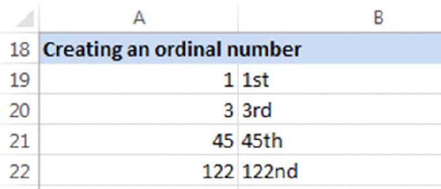
Figure 5.6 Using a formula to express a number as an ordinal.

Determining a column letter for a column number

This next formula returns a worksheet column letter (ranging from A to XFD) for the value contained in cell A1. For example, if A1 contains 29, the formula returns AC (the 29th column letter in a worksheet):

=LEFT(ADDRESS(1,A1,4),FIND(1,ADDRESS(1,A1,4))-1)

Note that the formula doesn’t check for a valid column number. In other words, if A1 contains a value less than 1 or greater than 16,384, the formula then returns an error. The following modification uses the IFERROR function to display text (Invalid Column) instead of an error value:

=IFERROR(LEFT(ADDRESS(1,A1,4),FIND(1,ADDRESS(1,A1,4))-1),"Invalid Column")

The IFERROR function was introduced in Excel 2007. For compatibility with versions prior to Excel 2007, use this formula:

=IF(ISERR(LEFT(ADDRESS(1,A1,4),FIND(1,ADDRESS(1,A1,4))-1)),

"Invalid Column",LEFT(ADDRESS(1,A1,4),FIND(1,ADDRESS(1,A1,4))-1))

Extracting a filename from a path specification

The following formula returns the filename from a full path specification. For example, if cell A1 contains c:\files\excel\myfile.xlsx, the formula returns myfile.xlsx:

=MID(A1,FIND("*",SUBSTITUTE(A1,"\","*",LEN(A1)-LEN(SUBSTITUTE(A1,"\",""))))+1,LEN(A1))

The preceding formula assumes that the system path separator is a backslash (\). It essentially returns all the text following the last backslash character. If cell A1 doesn’t contain a backslash character, the formula returns an error.

Note

In some cases, the Flash Fill feature can substitute for creating formulas that extract text from cells. See Chapter 16 for more information.

Extracting the first word of a string

To extract the first word of a string, a formula must locate the position of the first space character and then use this information as an argument for the LEFT function. The following formula does just that:

=LEFT(A1,FIND(" ",A1)-1)

This formula returns all the text prior to the first space in cell A1. However, the formula has a slight problem: it returns an error if cell A1 consists of a single word. A simple modification solves the problem by using an IFERROR function to check for the error:

=IFERROR(LEFT(A1,FIND(" ",A1)-1),A1)

For compatibility with versions prior to Excel 2007, use this formula:

=IF(ISERR(FIND(" ",A1)),A1,LEFT(A1,FIND(" ",A1)-1))

Extracting the last word of a string

Extracting the last word of a string is more complicated because the FIND function works from left to right only. Therefore, the problem rests with locating the last space character. The formula that follows, however, solves this problem. It returns the last word of a string (all the text following the last space character):

=RIGHT(A1,LEN(A1)-FIND("*",SUBSTITUTE(A1," ","*",LEN(A1)-LEN(SUBSTITUTE(A1," ","")))))

This formula, however, has the same problem as the first formula in the preceding section: it fails if the string does not contain at least one space character. The following modified formula uses the IFERROR function to avoid the error value:

=IFERROR(RIGHT(A1,LEN(A1)-FIND("*",SUBSTITUTE(A1," ","*",

LEN(A1)-LEN(SUBSTITUTE(A1," ",""))))),A1)

For compatibility with versions prior to Excel 2007, use this formula:

=IF(ISERR(FIND(" ",A1)),A1,

RIGHT(A1,LEN(A1)-FIND("*",SUBSTITUTE(A1," ","*",LEN(A1)-LEN(SUBSTITUTE(A1," ",""))))))

Extracting all but the first word of a string

The following formula returns the contents of cell A1, except for the first word:

=RIGHT(A1,LEN(A1)-FIND(" ",A1,1))

If cell A1 contains 2013 Operating Budget, the formula then returns Operating Budget.

This formula returns an error if the cell contains only one word. The following formula solves this problem and returns an empty string if the cell does not contain multiple words:

=IFERROR(RIGHT(A1,LEN(A1)-FIND(" ",A1,1)),"")

For compatibility with versions prior to Excel 2007, use this formula:

=IF(ISERR(FIND(" ",A1)),"",RIGHT(A1,LEN(A1)-FIND(" ",A1,1)))

Extracting first names, middle names, and last names

Suppose you have a list consisting of people’s names in a single column. You have to separate these names into three columns: one for the first name, one for the middle name or initial, and one for the last name. This task is more complicated than you may initially think because not every name in the column has a middle name or middle initial. However, you can still do it.

Note

The task becomes a lot more complicated if the list contains names with titles (such as Mrs. or Dr.) or names followed by additional details (such as Jr. or III). In fact, the following formulas will not handle these complex cases. However, they still give you a significant head start if you’re willing to do a bit of manual editing to handle the special cases.

All the formulas that follow assume that the name appears in cell A1.

You can easily construct a formula to return the first name:

=IFERROR(LEFT(A1,FIND(" ",A1)-1),A1)

Returning the middle name or initial is much more complicated because not all names have a middle initial. This formula returns the middle name or initial (if it exists); otherwise, it returns nothing:

=IF(LEN(A1)-LEN(SUBSTITUTE(A1," ",""))>1,

MID(A1,FIND(" ",A1)+1,FIND(" ",A1,FIND(" ",A1)+1)-(FIND(" ",A1)+1)),"")

Finally, this formula returns the last name:

=IFERROR(RIGHT(A1,LEN(A1)-FIND("*",SUBSTITUTE(A1," ","*",LEN(A1)-LEN(SUBSTITUTE (A1," ",""))))),"")

The formula that follows is a much shorter way to extract the middle name. This formula is useful if you use the other formulas to extract the first name and the last name. It assumes that the first name is in B1 and that the last name is in D1:

=IF(LEN(B1&D1)+2>=LEN(A1),"",MID(A1,LEN(B1)+2,LEN(A1)-LEN(B1&D1)-2)

As you can see in Figure 5.7, the formulas work fairly well. There are a few problems, however: notably, names that contain four “words.” But, as we mentioned earlier, you can clean up these cases.

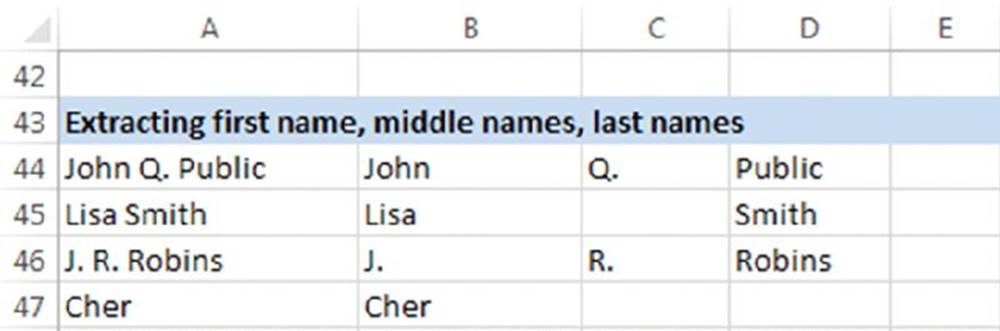
Figure 5.7 This worksheet uses formulas to extract the first name, middle name (or initial), and last name from a list of names in column A.

Cross-Ref

If you want to know how we created these complex formulas, see Chapter 21, “Creating Megaformulas.”

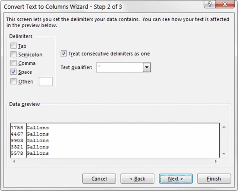
Splitting text strings without using formulas

In many cases, you can eliminate the use of formulas and use Excel’s Data ➜ Data Tools ➜ Convert Text to Columns command to parse strings into their component parts. Selecting this command displays Excel’s Convert Text to Columns Wizard (see the accompanying figure), which consists of a series of dialog boxes that walk you through converting a single column of data into multiple columns. Generally, you’ll want to select the Delimited option (in step 1) and use Space as the delimiter (in step 2).

Another string-splitting option is to use the Flash Fill feature.

Removing titles from names

You can use the formula that follows to remove four common titles (Mr., Dr., Ms., and Mrs.) from a name. For example, if cell A1 contains Mr. Fred Munster, the following formula would return Fred Munster:

=IF(OR(LEFT(A1,2)={"Mr","Dr","Ms"}),RIGHT(A1,LEN(A1)-(FIND(".",A1)+1)),A1)

Counting the number of words in a cell

The following formula returns the number of words in cell A1:

=LEN(TRIM(A1))-LEN(SUBSTITUTE((A1)," ",""))+1

The formula uses the TRIM function to remove excess spaces. It then uses the SUBSTITUTE function to create a new string (in memory) that has all the space characters removed. The length of this string is subtracted from the length of the original (trimmed) string to get the number of spaces. This value is then incremented by 1 to get the number of words.

Note that this formula returns 1 if the cell is empty. The following modification solves that problem:

=IF(LEN(A1)=0,0,LEN(TRIM(A1))-LEN(SUBSTITUTE(TRIM(A1)," ",""))+1)

Cross-Ref

Excel has many functions that work with text, but you’re likely to run into a situation in which the appropriate function just doesn’t exist. In such a case, you can often create your own worksheet function using VBA. Chapter 26 also contains a number of custom text functions written in VBA.