Excel 2016 for Windows Pivot Tables (2016)
2. Nesting Fields
You saw examples of one- and two-dimensional pivot tables in the preceding chapter, but Excel doesn’t limit the number of fields in a pivot table.
Adding Nested Fields
Each time that you add a new field, Excel subdivides, or nests, the current fields.
To add additional (nested) fields to a pivot table:
1. Select any cell in the pivot table.
Excel shows the PivotTable Fields pane.
2. In the PivotTable Fields pane, drag fields from the “Choose fields to add to report” list to the Rows or Columns boxes underneath.
The order of fields within a box determines their nesting order in the pivot table.
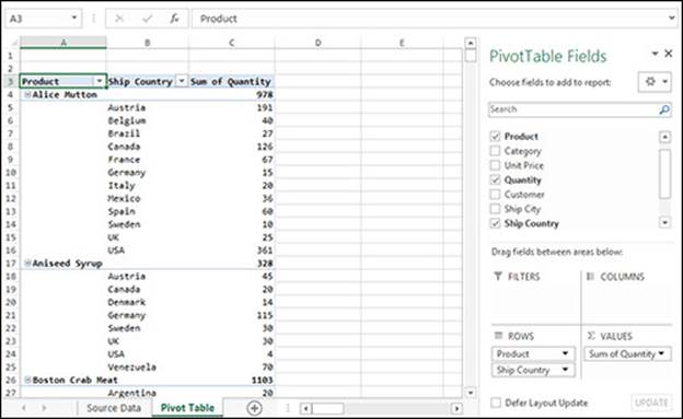
Consider a pivot table with the settings:
Rows: Product, Ship Country
Columns: (empty)
Values: Quantity (summarized by Sum)
Filters: (empty)
Each row in this pivot table shows the total units of a specific product shipped to a specific country.
Excessive nesting can make a pivot table uninformative or unwieldy. If the number of rows in a pivot table is close to the number of rows in the underlying source data, then that pivot table isn’t truly a summary. Another sign of an overnested pivot table is an excessive number of empty cells (wasted space). Consider a pivot table with the settings:
Rows: Category, Order Date
Columns: Ship Country
Values: Quantity (summarized by Sum)
Filters: (empty)
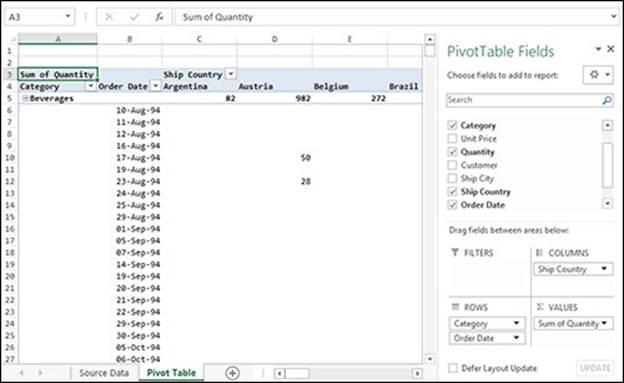
The rows in this pivot table are grouped by category and subdivided by order date. At 1605 rows (not counting subtotals or blank values), this pivot table isn’t much smaller than the source data (2155 rows). The problem is that few orders fall on the same date. And when they do, they’re usually for different product categories. Consequently, many rows show results for only a single order, rather than true totals. This pivot table is sparse (contains many empty cells) because each row is further broken up into columns by country.
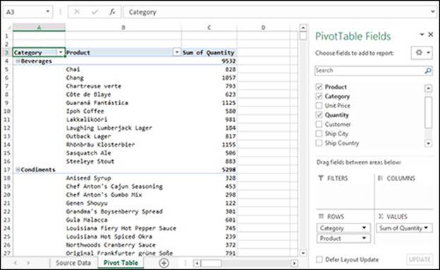
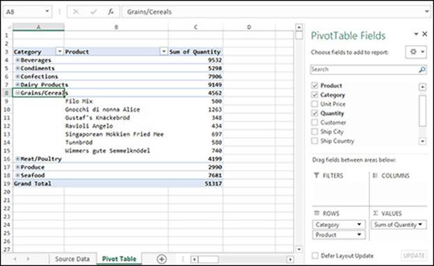
Nesting works best for closely related fields, such as Category and Product (each product falls in one category):
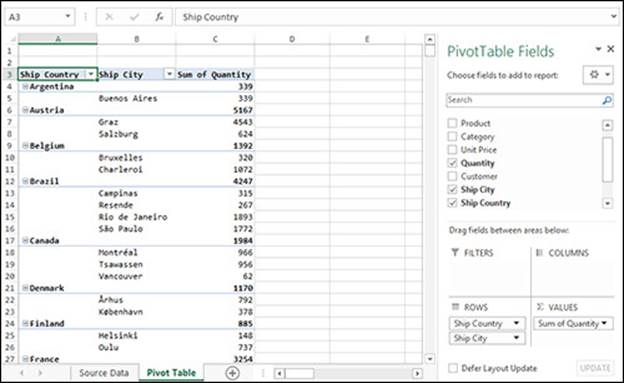
Or Ship Country and Ship City (each city is located in one country):
Make sure that you place the fields in the correct order in the Rows or Columns box; otherwise, you’ll get silly results. Consider a pivot table with the settings:
Rows: Product, Category
Columns: (empty)
Values: Quantity (summarized by Sum)
Filters: (empty)
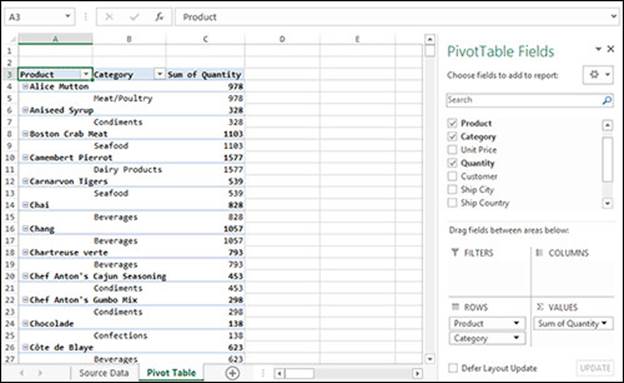
This pivot table groups the records by product and then subdivides the products by category, resulting in an unhelpful pivot table where each group contains a single subgroup (because each product falls in only one category). To fix this pivot table, swap the rows (that is, drag Product below Category in the Rows box).
To reorder fields in a pivot table:
1. Select any cell in the pivot table.
Excel shows the PivotTable Fields pane.
2. In the PivotTable Fields pane, drag fields up or down within a box, or click a field in a box and then choose Move Up or Move Down (or Move to Beginning or Move to End) from the pop-up menu.
Showing and Hiding Levels
You can show (expand) or hide (collapse) individual levels in nested rows or columns, concealing the parts of a pivot table that you don’t want to see. In a pivot table that nests Product within Category, for example, you can show only the products in a specific category and hide the rest.
To show or hide specific levels:
· Do any of the following:
» Click the plus (+) or minus (-) icon next to the level name in the pivot table (click again to toggle visibility).
» Double-click the cell containing the level name (double-click again to toggle visibility).
» Right-click the cell containing the level name and then choose Expand or Collapse from the Expand/Collapse submenu.
To show or hide all levels:
· Do any of the following:
» In the target field, right-click any cell containing a level name and then choose Expand Entire Field or Collapse Entire Field from the Expand/Collapse submenu.
» In the target field, select any cell containing a level name and then choose PivotTable Tools > Analyze tab > Active Field group > Expand Field or Collapse Field.
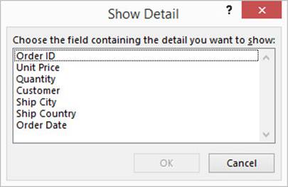
If you try to expand an innermost nested level, Excel opens the Show Detail dialog box listing all the fields not currently showing. If you select a field and then click OK, Excel adds another nested field to the pivot table.
All materials on the site are licensed Creative Commons Attribution-Sharealike 3.0 Unported CC BY-SA 3.0 & GNU Free Documentation License (GFDL)
If you are the copyright holder of any material contained on our site and intend to remove it, please contact our site administrator for approval.
© 2016-2026 All site design rights belong to S.Y.A.