Marketing Analytics: Data-Driven Techniques with Microsoft Excel (2014)

Part III. Forecasting

Chapter 11. Forecasting in the Presence of Special Events

Often special factors such as seasonality and promotions affect demand for a product. The Excel Regression tool can handle 15 independent variables, but many times that isn't enough. This chapter shows how to use the Excel Solver to build forecasting models involving up to 200 changing cells. The discussion is based on a student project (admittedly from the 1990s) that attempted to forecast the number of customers visiting the Eastland Plaza Branch of the Indiana University (IU) Credit Union each day. You'll use this project to learn how to forecast in the face of special factors.

Building the Basic Model

In this section you will learn how to build a model to forecast daily customer count at the Indiana University Credit Union. The development of the model should convince you that careful examination of outliers can result in more accurate forecasting.

The data collected for this example is contained in the original worksheet in the Creditunion.xlsx file and is shown in Figure 11.1. It is important to note that this data is before direct deposit became a common method to deposit paychecks. For each day of the year the following information is available:

· Month of the year

· Day of the week

· Whether the day was a faculty or staff payday

· Whether the day before or the day after was a holiday

Figure 11-1: Data for Credit Union example

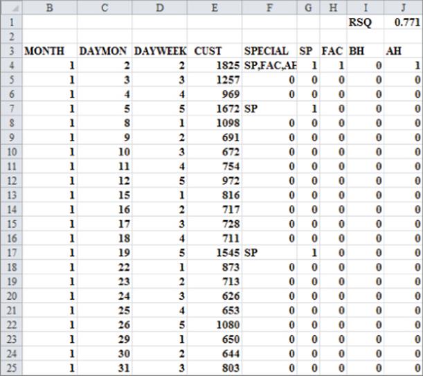
If you try to run a regression on this data by using dummy variables (as described in Chapter 10, “Using Multiple Regression to Forecast Sales,”) the dependent variable would be the number of customers arriving each day (the data in column E). Nineteen independent variables are needed:

· 11 to account for the month (12 months minus 1)

· 4 to account for the day of the week (5 business days minus 1)

· 2 to account for the types of paydays that occur each month

· 2 to account for whether a particular day follows or precedes a holiday

Microsoft Office Excel enables only 15 independent variables, so when a regression forecasting model requires more you can use the Excel Solver feature to estimate the coefficients of the independent variables. As you learned earlier, Excel's Solver can be used to optimize functions. The trick here is to apply Solver to minimize the sum of squared errors, which is the equivalent to running a regression. Because the Excel Solver allows up to 200 changing cells, you can use Solver in situations where the Excel Regression tool would be inadequate. You can also use Excel to compute the R-squared values between forecasts and actual customer traffic as well as the standard deviation for the forecast errors. To analyze this data, you create a forecasting equation by using a lookup table to “look up” the day of the week, the month, and other factors. Then you use Solver to choose the coefficients for each level of each factor that yields the minimum sum of squared errors. (Each day's error equals actual customers minus forecasted customers.) The following steps walk you through this process:

1. First, create indicator variables (in columns G through J) for whether the day is a staff payday (SP), faculty payday (FAC), before a holiday (BH), or after a holiday (AH). (Refer to Figure 11.1). For example, cells G4, H4, and J4 use 1 to indicate that January 2 was a staff payday, faculty payday, and after a holiday. Cell I4 contains 0 to indicate that January 2 was not before a holiday.

2. The forecast is defined by a constant (which helps to center the forecasts so that they will be more accurate), and effects for each day of the week, each month, a staff payday, a faculty payday, a day occurring before a holiday, and a day occurring after a holiday. Insert Trial values for all these parameters (the Solver changing cells) in the cell range O4:O26, as shown in Figure 11.2. Solver can then choose values that make the model best fit the data. For each day, the forecast of customer count will be generated by the following equation:

Predicted customer count=Constant+(Month effect)+(Day of week effect)+(Staff payday effect, if any)+(Faculty payday effect, if any)+(Before holiday effect, if any)+(After holiday effect, if any)

Figure 11-2: Changing cells for Credit Union example

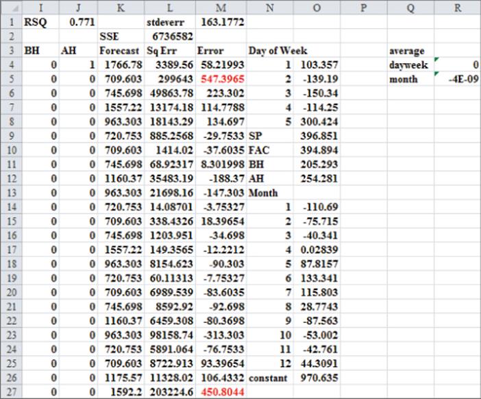
3. Using this model, compute a forecast for each day's customer count by copying the following formula from K4 to K5:K257:

$O$26+VLOOKUP(B4,$N$14:$O$25,2)+VLOOKUP(D4,$N$4:$O$8,2) +G4*$O$9+H4*$O$10+I4*$O$11+J4*$O$12.

Cell O26 picks up the constant term. VLOOKUP(B4,$N$14:$O$25,2) picks up the month coefficient for the current month, and VLOOKUP(D4,$N$4:$O$8,2) picks up the day of the week coefficient for the current week. =G4*$O$9+H4*$O$10+I4*$O$11+J4*$O$12 picks up the effects (if any) when the current day is SP, FAC, BH, or AH.

4. Copy the formula =(E4-K4)^2, from L4 to L5:L257 to compute the squared error for each day. Then, in cell L2, compute the sum of squared errors with the formula =SUM(L4:L257).

5. In cell R4, average the day of the week changing cells with the formula =AVERAGE(O4:O8), and in cell R5, average the month changing cells with the formula =AVERAGE(O14:O25). Later in this section you will add constraints to your Solver model which constrain the average month and day of the week effects to equal 0. These constraints ensure that a month or day of the week with a positive effect has a higher than average customer count, and a month or day of the week with a negative effect has a lower than average customer count.

6. Use the Solver settings shown in Figure 11.3 to choose the forecast parameters to minimize the sum of squared errors.

Figure 11-3: Solver settings for Credit Union example

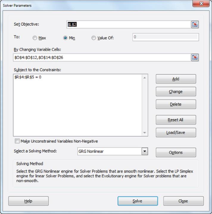
The Solver model changes the coefficients for the month, day of the week, BH, AH, SP, FAC, and the constant to minimize the sum of square errors. It also constrains the average day of the week and month effect to equal 0. The Solver enables you to obtain the results shown in Figure 11.2. These show that Friday is the busiest day of the week and June is the busiest month. A staff payday raises the forecast (all else being equal—in the Latin, ceteris paribus) by 397 customers.

Evaluating Forecast Accuracy

To evaluate the accuracy of the forecast, you compute the R² value between the forecasts and the actual customer count in cell J1. You use the formula =RSQ(E4:E257,K4:K257) to do this. This formula computes the percentage of the actual variation in customer count that is explained by the forecasting model. The independent variables explain 77 percent of the daily variation in customer count.

You can compute the error for each day in column M by copying the formula =E4–K4 from M4 to M5:M257. A close approximation to the standard error of the forecast is given by the standard deviation of the errors. This value is computed in cell M1 by using the formula =STDEV(M4:M257). Thus, approximately 68 percent of the forecasts should be accurate within 163 customers, 95 percent accurate within 326 customers, and so on.

After you evaluate the accuracy of your forecasts and compute the error, you will want to try and spot any outliers. Recall that an observation is an outlier if the absolute value of the forecast error exceeds two times the standard error of the regression. To locate the outliers, perform the following steps:

1. Select the range M4:M257, and then click Conditional Formatting on the Home tab.

2. Select New Rule and in the New Formatting Rule dialog box, choose Use a Formula to Determine Which Cells to Format.

3. Fill in the rule description in the dialog box, as shown in Figure 11.4.

Figure 11-4: Highlighting outliers

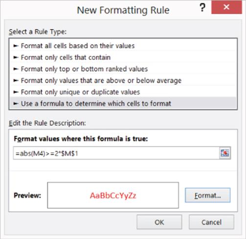
This procedure essentially copies the formula from M4 to M5:M257 and formats the cell in red if the formula is true. This ensures that all outliers are highlighted in red.

After choosing a format with a red font, the conditional formatting settings display in red any error whose absolute value exceeds 2 * (standard deviation of errors). Looking at the outliers, you see that the customer count for the first three days of the month is often under forecast. Also, during the second week in March (spring break), the data is over forecast, and the day before spring break, it is greatly under forecast.

Refining the Base Model

To remedy this problem, the 1st three days worksheet from the Creditunion.xlsx file shows additional changing cells for each of the first three days of the month and for spring break and the day before spring break. There are also additional trial values for these new effects in cells O26:O30. By copying the following formula from K4 to K5:K257 you can include the effects of the first three days of the month:

=$O$25+VLOOKUP(B4,$N$13:$O$24,2)+VLOOKUP(D4,$N$4:$O$8,2)+G4*$O$9+H4* $O$10+I4*$O$11+J4*$O$12+IF(C4=1,$O$26,IF(C4=2,$O$27,IF(C4=3,$O$28,0)))

NOTE

The term =IF(C4=1,$O$26,IF(C4=2,$O$27,IF(C4=3,$O$28,0))) picks up the effect of the first three days of the month. For example, if Column C indicates that the day is the first day of the month, the First Day of the Month effect from O26 is added to the forecast.

You can now manually enter the spring break coefficients in cells K52:K57. For this example, you add +O29 to the formula in cell K52 and +O30 in cells K52:K57.

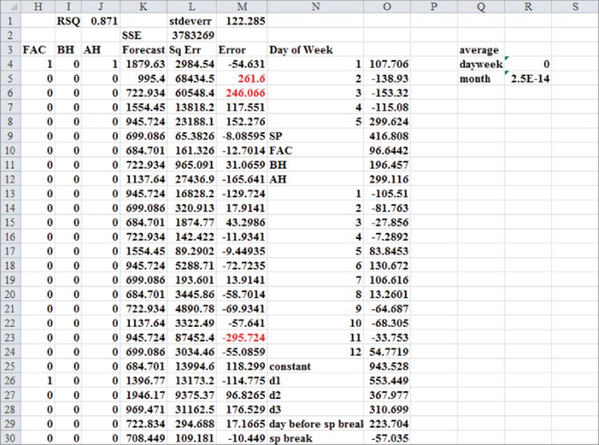
After including the new changing cells in the Solver dialog box, you can find the results shown in Figure 11.5. Notice that the first three days of the month greatly increase customer count (possibly because of government support and Social Security checks) and that spring break reduces customer count. Figure 11.5 also shows the improvement in forecasting accuracy. The R² value is improved to 87 percent and the standard error is reduced to 122 customers.

Figure 11-5: Credit Union model including Spring Break and First Three Days of Month factors

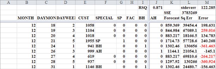
By looking at the forecast errors for the week 12/24 through 12/31 (see Figure 11.6), you see that you've greatly over forecasted the customer counts for the days in this week. You've also under forecasted customer counts for the week before Christmas. Further examination of the forecast errors (often called residuals) also shows the following:

· Thanksgiving is different than a normal holiday in that the credit union is far less busy than expected the day after Thanksgiving.

· The day before Good Friday is busy because people leave town for Easter.

· Tax day (April 16) is also busier than expected.

· The week before Indiana University starts fall classes (last week in August) is not busy, possibly because many staff and faculty take a “summer fling vacation” before the hectic onrush of the fall semester.

Figure 11-6: Pre- and post-Christmas forecasts are way off!

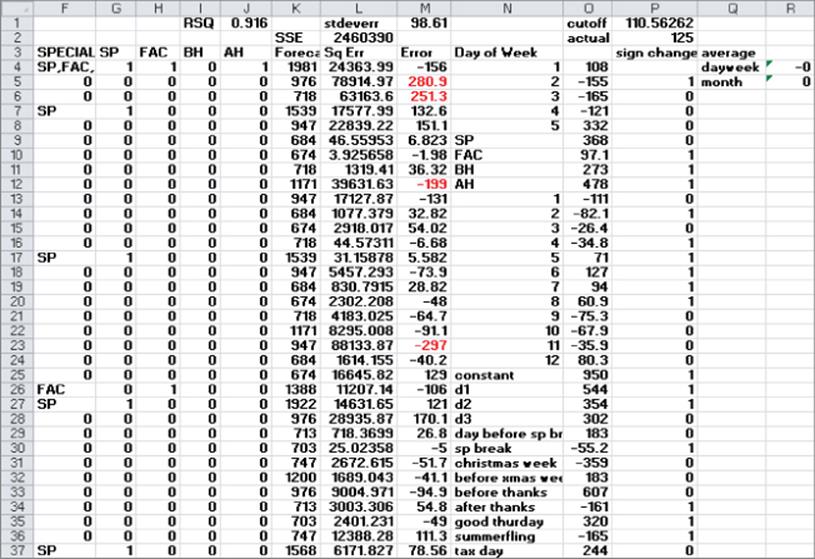
In the Christmas week worksheet, these additional factors are included as changing cells in the forecast models. After adding the new parameters as changing cells, run Solver again. The results are shown in Figure 11.7. The R² is up to 92 percent and the standard error is down to 98.61 customers! Note that the post-Christmas week reduced the daily customer count by 359; the day before Thanksgiving added 607 customers; the day after Thanksgiving reduced customer count by 161, and so on.

Figure 11-7: Final forecast model

Notice that you improve the forecasting model by using outliers. If your outliers have something in common (such as being the first three days of the month), include the common factor as an independent variable and your forecasting error drops.

The forecasting model can provide useful insights in a variety of situations. For instance, a similar analysis was performed to predict daily customer count for dinner at a major restaurant chain. The special factors corresponded to holidays. Super Bowl Sunday was the least busy day and Valentine's Day and Mother's Day were the busiest. Also, Saturday was the busiest day of the week for dinner, and Friday was the busiest day of the week for lunch. Using the model described in this section, after adjusting for all other factors the restaurant chain found the following:

· On Saturdays 192 more people than average ate dinner and on Mondays 112 fewer people than average ate dinner.

· On Super Bowl Sunday 212 fewer people than average ate dinner and on Mother's Day and Valentine's Day 350 more people ate dinner. Since an average of 401 people ate dinner daily, the model shows that business almost doubles on Mother's Day and Valentine's Day, and business is cut in half on Super Bowl Sunday.

In contrast, for pizza delivery companies such as Domino's, Super Bowl Sunday is the busiest day of the year. Given daily counts of delivered pizzas, it would be easy to come up with an accurate estimate of the effect of Super Bowl Sunday on pizza deliveries.

Checking the Randomness of Forecast Errors

A good forecasting method should create forecast errors or residuals that are random. Random errors mean that the errors exhibit no discernible pattern. If forecast errors are random, the sign of your errors should change (from plus to minus or minus to plus) approximately half the time. Therefore, a commonly used test to evaluate the randomness of forecast errors is to look at the number of sign changes in the errors. If you have n observations, nonrandomness of the errors is indicated if you find either fewer than or more than n changes in sign. The Christmas weekworksheet, as shown in Figure 11.7, determines the number of sign changes in the residuals by copying the formula =IF(M5*M4<0,1,0) from cell P5 to P6:P257. A sign change in the residuals occurs if, and only if, the product of two consecutive residuals is negative. Therefore, the formula yields 1 whenever a change in the sign of the residuals occurs. In this worksheet example, there were 125 changes in sign. Cell P1 computes changes in sign as the cutoff for nonrandom residuals. Therefore there are random residuals here.

Summary

In this chapter you learned the following:

· The Excel Solver can be used to mimic regression analysis and work around the 15 independent variable limitations of Excel's Regression tool.

· Using the Excel Solver you can often forecast daily demand with the model Base Level + Day of Week Effect + Month Effect + Effect of Special Factors.

· You can use outliers to spot omitted special factors.

· If the signs of residuals change much less than half the time, then forecast errors are not random.

Exercises

1. How can you use the techniques outlined in this chapter to predict the daily sales of pens at Staples?

2. If you had several years of data, how would you incorporate a trend in the analysis?

3. The file Dinner.xls contains a model to predict daily dinner sales at a well-known chain restaurant. Column Q of the worksheet outliers removed contains the final forecast equation.

(a) Explain in words the equation used to forecast daily dinner sales.

(b) Explain how the day of the week affects dinner sales.

(c) Explain how the time of year affects dinner sales.

(d) Explain the special factors that affect dinner sales.

(e) What other data might you want to collect to improve forecast accuracy?

4. The file Promotiondata.xlsx contains monthly sales (in pounds) of ice cream at a Kroger's supermarket for three years. The file also tells you when promotions occurred. Promotions are known to increase sales during the month of the promotion but decrease sales during the month after the promotion. Develop a model that can be used to predict monthly ice cream sales. Hint: Add a term to your model involving the month number; the coefficient of this term will model the trend in ice cream sales.

(a) What percentage of variation in ice cream sales is explained by your model?

(b) Fill in the blank: 95 percent of forecasts for monthly sales will be accurate within ________.

(c) What month appears to be the best for ice cream sales?

(d) Describe the trend of ice cream sales.

(e) Describe the effect of a promotion on ice cream sales.