Marketing Analytics: Data-Driven Techniques with Microsoft Excel (2014)
Part III. Forecasting
Chapter 12. Modeling Trend and Seasonality
Whether the marketing analyst works for a car manufacturer, airline, or consumer packaged goods company, she often must forecast sales of her company's product. Whatever the product, it is important to understand the trends (either upward or downward) and seasonal aspects of the product's sales. This chapter discusses how to determine the trends and seasonality of product sales. Using monthly data on U.S. air passenger miles (2003–2012) you will learn how to do the following:
· Use moving averages to eliminate seasonality to easily see trends in sales.
· Use the Solver to develop an additive or multiplicative model to estimate trends and seasonality.
Using Moving Averages to Smooth Data and Eliminate Seasonality
Moving averages smooth out noise in the data. For instance, suppose you work for Amazon.com and you are wondering whether sales are trending upward. For each January sales are less than the previous month (December sales are always high because of Christmas), so the unsuspecting marketing analyst might think there is a downward trend in sales during January because sales have dropped. This conclusion is incorrect, though, because it ignores the fact that seasonal influences tend to drop January sales below December sales. You can use moving averages to smooth out seasonal data and better understand the trend and seasonality characteristics of your data.
NOTE
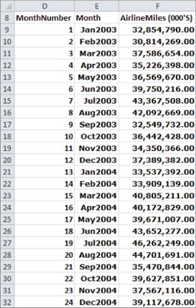
All work in this chapter uses the file airlinemiles.xlsx, which contains monthly airlines miles (in thousands) traveled in the United States during the period from January 2003 through April 2012. A sample of this data is shown in Figure 12.1.
Figure 12-1: US airline miles
To further illustrate the concept of moving averages, take a look at the graph of United States airline miles shown in Figure 12.2. To obtain this graph select the data from the Moving average worksheet of the airlinemiles.xlsx file in the range E8:F120 and select Insert &cmdarr; Charts &cmdarr; Scatter and choose the second option (Scatter with Smooth Lines and Markers). You obtain the graph shown in Figure 12.2.
Figure 12-2: Graph of US airline miles
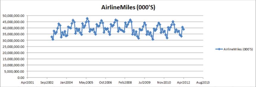
Due to seasonality (primarily because people travel more in the summer), miles traveled usually increase during the summer and then decrease during the winter. This makes it difficult to ascertain the trend in airline travel. Graphing the moving average of airline miles can help to better understand the trend in this data. A 12-month moving average, for example, graphs the average of the current month's miles and the last 11 months. Because moving averages smooth out noise in the data, you can use a 12-month moving average to eliminate the influence of seasonality. This is because a 12-month moving average includes one data point for each month. When analyzing a trend in quarterly data, you should plot a four-quarter moving average.
To overlay a 12-month moving average on the scatterplot, you return to an old friend, the Excel Trendline. Right-click the data series and select Add Trendline… Choose Moving Average and select 12 periods. Then you can obtain the trendline, as shown in Figure 12.3.
Figure 12-3: Moving average trendline
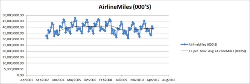
The moving average trendline makes it easy to see how airline travel trended between 2003 and 2012. You can now see the following:
· In 2003 and 2004 there was a sharp upward trend in airline travel (perhaps a rebound from 9/11).
· In 2005–2008 airline travel appeared to stagnate.
· In late 2008 there was a sharp drop in airline travel, likely due to the financial crisis.
· In 2010 a slight upward trend in air travel occurred.
The next section uses the Excel Solver to quantify the exact nature of the trend in airline miles and also to learn how to determine how seasonality influences demand for air travel.
An Additive Model with Trends and Seasonality
Based on the previous section's discussion it should be clear that to accurately forecast sales when the data has seasonality and trends, you need to identify and separate these from the data series. In this section you learn how this process can be modeled using Excel's Solver. These analyses enable you to identify and separate between the baseline, seasonality, and trend components of a data series.
When predicting product sales, the following additive model is often used to estimate the trend and seasonal influence of sales:
1 ![]()
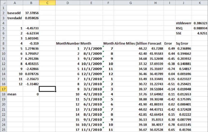
In Equation (1) you need to estimate the base, trend, and seasonal index for each month of the year. The work for this appears in the Additive trend worksheet (see Figure 12.4). To simplify matters the data is rescaled in billions of miles. The base, trend, and seasonal index may be described as follows:
· Base: The base is the best estimate of the level (without seasonality) of monthly airline miles at the beginning of the observed time period.
· Trend: The trend is the best estimate of the monthly rate of increase in airline miles traveled. A trend of 5, for example, would mean that the level of airline travel is increasing at a rate of 5 billion miles per month.
· Seasonal Index: Each month of the year has a seasonal index to reflect if travel during the month tends to be higher or lower than average. A seasonal index of +5 for June would mean, for example, that June airline travel tends to be 5 billion miles higher than an average month.
Figure 12-4: Additive trend model
NOTE
The seasonal indices must average to 0.
To estimate base, trend, and seasonal indices, you need to create formulas based on trial values of the parameters in Column H. Then in Column I, you will determine the error for each month's forecast, and in Column J, you compute the squared error for each forecast. Finally, you use the Solver to determine the parameter values that minimize squared errors. To execute this estimation process, perform the following steps:
1. Enter trial values of the base and trend in cells B2 and B3. Name cell B2 baseadd and cell B3 trend.
2. Enter trial seasonal indices in the range B5:B16.
3. In cell B18, average the seasonal indices with the formula =AVERAGE(B5:B16).The Solver model can set this average to 0 to ensure the seasonal indices average to 0.
4. Copy the formula =baseadd+trend*D9+VLOOKUP(F9,$A$5:$B$16,2) from H9 to H10:H42 to compute the forecast for each month.
5. Copy the formula =G9-H9 from I9 to I10:I42 to compute each month's forecast error.
6. Copy the formula =(I9^2) from J9 to J10:J42 to compute each month's squared error.
7. In cell K6, compute the Sum of Squared Errors (SSE) using the formula =SUM(J9:J42).
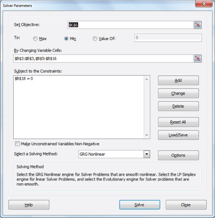
8. Now set up the Solver model, as shown in Figure 12.5. Change the parameters to minimize SSE and constrain the average of the seasonal indices to 0. Do not check the non-negative box because some seasonal indices must be negative. The forecasting model of Equation (1) is a linear forecasting model because each unknown parameter is multiplied by a constant. When the forecasts are created by adding together terms that multiply changing cells by constants, the GRG Solver Engine always finds a unique solution to the least square minimizing parameter estimates for a forecasting model.
Figure 12-5: Additive trend Solver model
Refer to the data shown in Figure 12.4 and you can make the following estimates:
· At the beginning of July 2009, the base level of airline miles is 37.38 billion.
· An upward trend in airline miles is 59 billion miles per month.
· The busiest month is July (6.29 billion miles above average) and the slowest month is February with 6.62 billion miles below average.
Cell K5 uses the formula =RSQ(G9:G42,H9:H42) to show that the model explains 98.9 percent of the variation in miles traveled. Cell K4 also computes the standard deviation of the errors (989 billion) with the formula =STDEV(I9:I42). You should expect 95 percent of the predictions to be accurate within 2 * 0.386 = 0.772 billion miles. Looking at Column I, no outliers are found.
A Multiplicative Model with Trend and Seasonality
When predicting product sales, the following multiplicative model is often used to estimate the trend and seasonal influence of sales:
2 ![]()
As in the additive model, you need to estimate the base, trend, and seasonal indices. In Equation (2) the trend and seasonal index have different meanings than in the additive model.
· Trend: The trend now represents the percentage monthly increase in the level of airline miles. For example, a trend value of 1.03 means monthly air travel is increasing 3 percent per month, and a trend value of .95 means monthly air travel is decreasing at a rate of 5 percent per month. If per period growth is independent of the current sales value, the additive trend model will probably outperform the multiplicative trend model. On the other hand, if per period growth is an increasing function of current sales, the multiplicative trend model will probably outperform the additive trend model.
· Seasonal Index: The seasonal index for a month now represents the percentage by which airline travel for the month is above or below an average month. For example, a seasonal index for July of 1.16 means July has 16 percent more air travel than an average month, whereas a seasonal index for February of .83 means February has 17 percent less air travel than an average month. Of course, multiplicative seasonal indices must average to 1. This is because months with above average sales are indicated by a seasonal index exceeding 1, while months with below average sales are indicated by a seasonal index less than 1.
The work for this equation appears in the Multiplicative trend worksheet. All the formulas are the same as the additive model with the exception of the monthly forecasts in Column H. You can implement Equation (2) by copying the formula =base*(trend^D9)*VLOOKUP(F9,$A$5:$B$16,2)from H9 to H10:H42.
The forecasting model in Equation (2) is a nonlinear forecasting model because you can raise the trend to a power and multiply, rather than add terms involving the seasonal indices. For nonlinear forecasting models, the GRG Solver Engine often fails to find an optimal solution unless the starting values for the changing cells are close to the optimal solution. The remedy to this issue is as follows:
1. In Solver select Options, and from the GRG tab, select Multistart. This ensures the Solver will try many (between 50 and 200) starting solutions and find the optimal solution from each starting solution. Then the Solver reports the “best of the best” solutions.
2. To use the Multistart option, input lower and upper bounds on the changing cells. To speed up solutions, these bounds should approximate sensible values for the estimated parameters. For example, a seasonal index will probably be between 0 and 3, so an upper bound of 100 would be unreasonable. As shown in Figure 12.6, you can choose an upper bound of 3 for each seasonal index and an upper bound of 2 for the trend. For this example, choose an upper bound of 100 for the base.
Figure 12-6: Solver window for multiplicative trend model
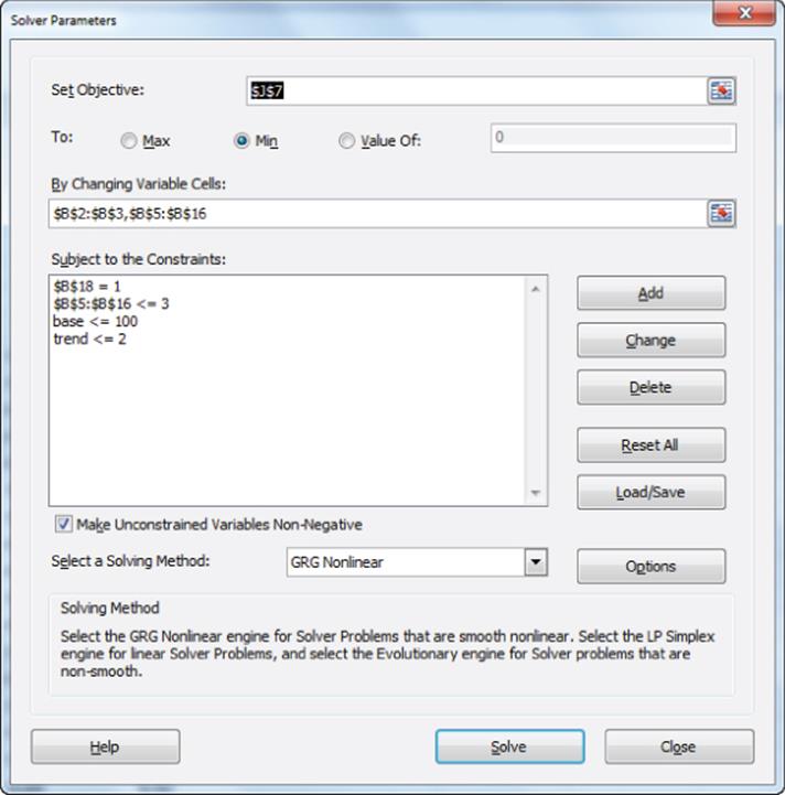
3. Cell B18 averages the seasonal indices, so in the Solver window add the constraint $B$18 =1 to ensure that the seasonal indices average to 1.
4. Select Solve, and the Solver will then find the optimal solution (refer to Figure 12.7).
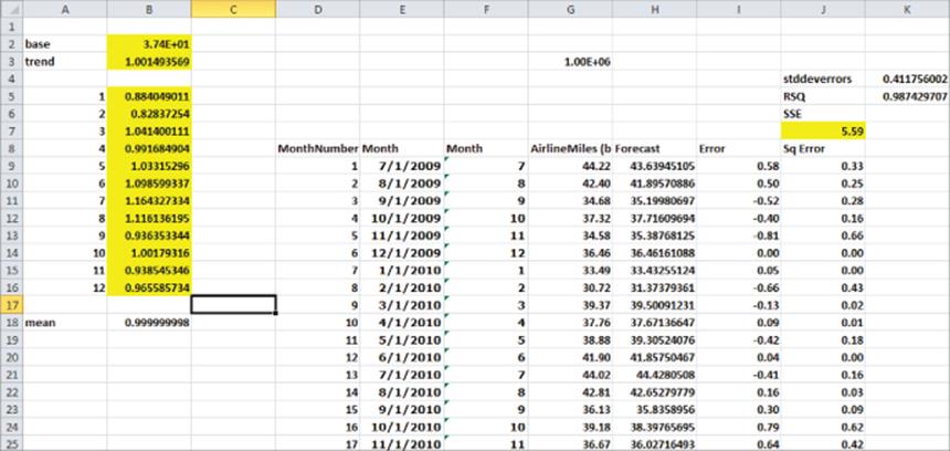
Figure 12-7: Multiplicative trend model
NOTE
If the Solver assigns a changing cell, a value near its lower or upper bound should be relaxed. For example, if you set the upper bound for the base to 30, the Solver will find a value near 30, thereby indicating the bound should be relaxed.
From the optimal Solver solution you find the following:
· The estimated base level of airline miles is 37.4 billion.
· You can estimate airline miles increase at a rate of 0.15 percent per month or 1.0014912 – 1 = 1.8 percent per year.
· The busiest month for the airlines is July, when miles traveled are 16 percent above average, and the least busy month is February, during which miles traveled are 17 percent below average.
A natural question is whether the additive or multiplicative model should be used to predict airline miles for future months. Because the additive model has a lower standard deviation of residuals, you should use the additive model to forecast future airline miles traveled.
Summary
In this chapter you learned the following:
· Using a 12-month or 4-quarter moving average chart enables you to easily see the trend in a product's sales.
· You can often use seasonality and trend to predict sales by using the following equation:
![]()
· You can often use the following equation to predict sales of a product:
![]()
Exercises
The following exercises use the file airlinedata.xlsx, which contains monthly U.S. domestic air miles traveled during the years 1970–2004.
1. Determine the trend and seasonality for the years 1970–1980.
2. Determine the trend and seasonality for the years 1981–1990.
3. Determine the trend and seasonality for the years 1995–2004.
All materials on the site are licensed Creative Commons Attribution-Sharealike 3.0 Unported CC BY-SA 3.0 & GNU Free Documentation License (GFDL)
If you are the copyright holder of any material contained on our site and intend to remove it, please contact our site administrator for approval.
© 2016-2026 All site design rights belong to S.Y.A.