Marketing Analytics: Data-Driven Techniques with Microsoft Excel (2014)
Part IV. What do Customers Want?
Chapter 17. Logistic Regression
Many marketing problems and decisions deal with understanding or estimating the probability associated with certain events or behaviors, and frequently these events or behaviors tend to be dichotomous—that is, of one type or of another type. When this is the case, the marketing analyst must predict a binary dependent variable (one that assumes the value 0 or 1, representing the inherent dichotomy) from a set of independent variables. Some examples follow:
· Predicting from demographic behavior whether a person will (dependent variable = 1) or will not (dependent variable = 0) subscribe to a magazine or use a product.
· Predicting whether a person will (dependent variable = 1) or will not (dependent variable = 0) respond to a direct mail campaign. Often the independent variables used are recency (time since last purchase), frequency (how many orders placed in last year), and monetary value (total amount purchased in last year.
· Predicting whether a cell phone customer will “churn” (dependent variable = 1) by end of year and switch to another carrier. The dependent variable = 0 if you retain the customer. You will see in Chapters 19, “Calculating Lifetime Customer Value,” and 20, “Using Customer Value to Value a Business,” that a reduction in churn can greatly increase the value of a customer to the company.
In this chapter you learn how to use the widely used tool of logistic regression to predict a binary dependent variable. You learn the following:
· Why multiple linear regression is not equal to the task of predicting a binary dependent variable
· How the Excel Solver may be used to implement the technique of maximum likelihood to estimate a logistic regression model
· How to interpret the coefficients in a logistic regression model
· How Palisade's StatTools program can easily be used to estimate a logistic regression model and test hypotheses about the individual coefficients
Why Logistic Regression Is Necessary
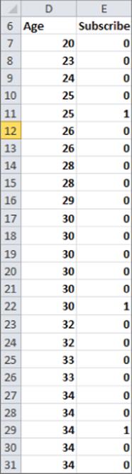
To explain why you need logistic regression, suppose you want to predict the chance (based on the person's age) that a person will subscribe to a magazine. The linear regression worksheet in the subscribers.xlsx file provides the age and subscription status (1 = subscriber, 0 = nonsubscriber) for 41 people. Figure 17.1 displays a subset of this data.
Figure 17-1: Age and subscriber status
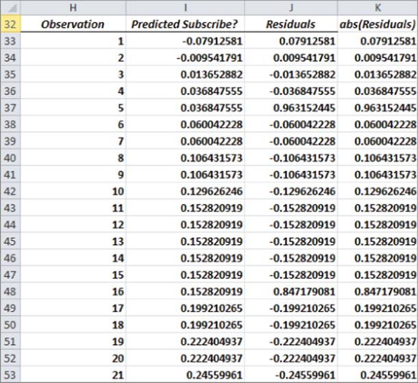
Using this data, you can run a linear regression to predict a subscriber's status from the subscriber's age. The Y-range is E6:E47 and the X-range is E6:E47. Check the residual box because you will soon see that the residuals indicate two of the key assumptions (from Chapter 10, “Using Multiple Regression to Forecast Sales”) of regression are violated. Figure 17.2 and Figure 17.3 show the results of running this regression.
Figure 17-2: Flawed linear regression
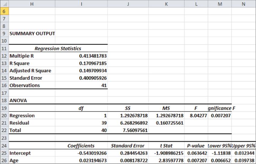
Figure 17-3: Residuals for flawed regression
From Figure 17.2 you can find the following equation:
![]()
Using the Residuals column shown in Figure 17.3, you can see three problems with this equation.
· Some observations predicted a negative subscriber status. Because the subscriber status must be 0 or 1, this is worrisome. Particularly, if you want to predict the probability that a person is a subscriber, a negative probability does not make sense.
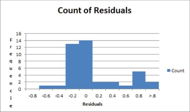
· Recall from Chapter 10 that the residuals should indicate that the error term in a regression should be normally distributed. Figure 17.4, however, shows a histogram of the residuals in which this is not the case.
Figure 17-4: Histogram of residuals
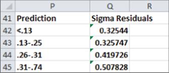
· Figure 17.5 gives the standard deviation of the residuals as a function of the predicted value of the subscriber variable. The spread of the residuals is not independent of the predicted value of the dependent variable. This implies that the assumption of homoscedasticity is violated. It can be shown that the variance of the error term in predicting a binary dependent variable is largest when the probability of the dependent variable being 1 (or 0) is near .5 and decreases as this probability moves away from .5.
Figure 17-5: Residual spread as function of predicted dependent variable
The Logistic Regression Model, described in the following section, resolves these three problems.
Logistic Regression Model
Let p = probability and a binary dependent variable = 1. In virtually all situations it appears that the relationship between p and the independent variable(s) is nonlinear. Analysts have often found that the relationship in Equation 1 does a good job of explaining the dependence of a binary-dependent variable on an independent variable.
1 ![]()
The transformation of the dependent variable described by Equation 1 is often called the logit transformation.
In this magazine example, Equation 1 takes on the following form:
2 ![]()
In Equation 2, ![]() is referred to as the log odds ratio, because
is referred to as the log odds ratio, because ![]() (the odds ratio) is the ratio of the probability of success (dependent variable = 1) to the probability of failure (dependent variable = 0.)
(the odds ratio) is the ratio of the probability of success (dependent variable = 1) to the probability of failure (dependent variable = 0.)
If you take e to both sides of Equation 2 and use the fact that eLn x = x, you can rewrite Equation 2 as one of the following:
3 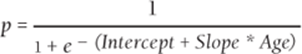
or
4 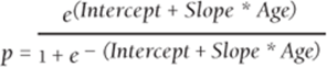
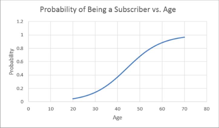
Equation 3 is often referred to as the logistic regression model (or sometimes the logit regression model) because the function ![]() is known as the logistic function. Note that 0 < p < 1. Because p is a probability, this is desirable. In the next section you find the best estimate of slope and intercept to be slope = 0.1281 and intercept = 5.662. Substituting these values into Equation 3 shows that as a function of age, a person's chance of being a subscriber varies according to the S-curve, as shown in Figure 17.6. Note that this relationship is highly nonlinear.
is known as the logistic function. Note that 0 < p < 1. Because p is a probability, this is desirable. In the next section you find the best estimate of slope and intercept to be slope = 0.1281 and intercept = 5.662. Substituting these values into Equation 3 shows that as a function of age, a person's chance of being a subscriber varies according to the S-curve, as shown in Figure 17.6. Note that this relationship is highly nonlinear.
Figure 17-6: S-curve for Being a Subscriber versus Age relationship
Maximum Likelihood Estimate of Logistic Regression Model
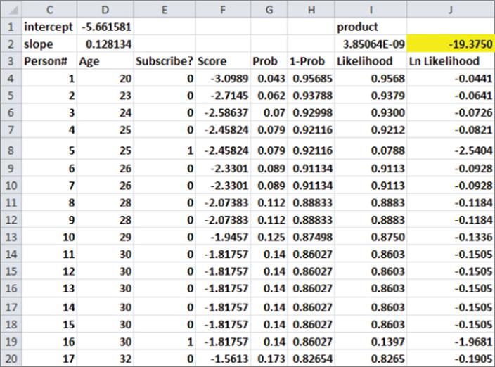
This section demonstrates how to use the maximum likelihood method to estimate the coefficients in a logistic regression model. Essentially, in the magazine example, the maximum likelihood estimation chooses the slope and intercept to maximize, given the age of each person, the probability or likelihood of the observed pattern of subscribers and nonsubscribers. For each observation in which the person was a subscriber, the probability that the person was a subscriber is given by Equation 4, and for each observation in which the person is not a subscriber, the probability that the person is not a subscriber is given by 1 – (right side of Equation 4). If you choose slope and intercept to maximize the product of these probabilities, then you are “maximizing the likelihood” of what you have observed. Unfortunately, the product of these probabilities proves to be a small number, so it is convenient to maximize the natural logarithm of this product. The following equation makes it easy to maximize the log likelihood.
5 ![]()
The work for this equation is shown in Figure 17.7 and is located in the data worksheet.
Figure 17-7: Maximum likelihood estimation
To perform the maximum likelihood estimation of the slope and intercept for the subscriber example, proceed as follows:
1. Enter trial values of the intercept and slope in D1:D2, and name D1:D2 using Create from Selection.
2. Copy the formula =intercept+slope*D4 from F4 to F5:F44, to create a “score” for each observation.
3. Copy the formula =EXP(F4)/(1+EXP(F4)) from G4 to G5:G44 to use Equation 4 to compute for each observation the estimated probability that the person is a subscriber.
4. Copy the formula =1-G4 from H4 to H5:H44 to compute the probability of the person not being a subscriber.
5. Copy the formula =IF(E4=1,G4,1-G4) from I4 to I5:I44 to compute the likelihood of each observation.
6. In I2 the formula =PRODUCT(I5:I44) computes the likelihood of the observed subscriber and nonsubscriber data. Note that this likelihood is a small number.
7. Copy the formula =LN(I4) from J4 to J5:J44, to compute the logarithm of each observation's probability.
8. Use Equation 5 in cell J2 to compute the Log Likelihood with the formula =SUM(J4:J44).
9. Use the Solver window (in Figure 17.8), to determine the slope and intercept that maximize the Log Likelihood.
Figure 17-8: Maximum Likelihood Solver window
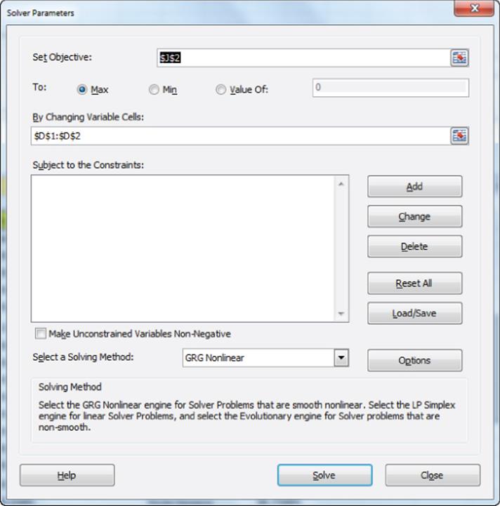
10. Press Solve and you find the maximum likelihood estimates of slope = -5.661 and Intercept = 0.1281.
Using a Logistic Regression to Estimate Probabilities
You can use logistic regression with Equation 4 to predict the chance that a person will be a subscriber based on her age. For example, you can predict the chance that a 44-year-old is a subscriber with the following equation:
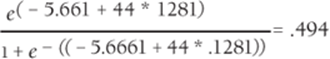
Since e raised to any power is a positive number, you can see that unlike ordinary least squares regression, logistic regression can never give a negative number for a probability. In Exercise 7 you will show that logistic regression also resolves the problems of heteroscedasticity and non-normal residuals.
Interpreting Logistic Regression Coefficients
In a multiple linear regression, you know how to interpret the coefficient of an independent variable: If βi is the coefficient of an independent variable xi, then a unit increase in the independent variable can increase the dependent variable by βi. In a logistic regression, the interpretation of the coefficient of an independent variable is much more complex: Suppose in a logistic regression βi is the coefficient of an independent variable xi. It can be shown (see Exercise 6) that a unit increase in xi increases the odds ratio ![]() by eβi percent. In the magazine example, this means that for any age a one-year increase in age increases the odds ratio by e.1281 = 13.7 percent.
by eβi percent. In the magazine example, this means that for any age a one-year increase in age increases the odds ratio by e.1281 = 13.7 percent.
Using StatTools to Estimate and Test Logistic Regression Hypotheses
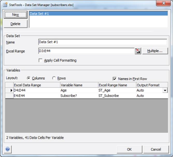
Chapter 10 explains how easy it is to use the Excel Analysis ToolPak to estimate a multiple linear regression and test relevant statistical hypotheses. The last section showed that it is relatively easy to use the Excel Solver to estimate the coefficients of a logistic regression model. Unfortunately, it is difficult to use “garden variety” Excel to test logistic regression statistical hypotheses. This section shows how to use Palisade's add-in StatTools (a 15-day trial version is downloadable from Palisade.com) to estimate a logistic regression model and test hypotheses of interest. You can also use full-blown statistical packages such as SAS or SPSS to test logistic regression statistical hypotheses. The work for this section is in the data worksheet of the subscribers.xlsx workbook.
Running the Logistic Regression with StatTools
To start StatTools simply click it on the desktop or start it from the All Programs menu. After bringing up StatTools, proceed as follows:
1. Choose Data Set Manager from the StatTools Toolbar, and select the data range (D3:E44), as shown in Figure 17.9.
Figure 17-9: Selecting data for the subscriber example
2. From the Regression and Classification menu, select Logistic Regression…, and fill in the dialog box, as shown in Figure 17.10.
Figure 17-10: Dialog box for Logistic Regression
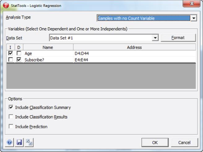
This dialog box tells StatTools to use Logistic Regression to predict Subscribe from Age. After selecting OK you can obtain the StatTools printout, as shown in Figure 17.11.
Figure 17-11: StatTools logistic regression output
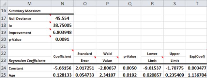
Interpreting the StatTools Logistic Regression Output
It is not necessary for the marketing analyst to understand all numbers in the StatTools output, but the key parts of the output are explained here:
· The maximum likelihood estimates of the intercept (-5.661 in cell N24) and slope (0.1281 in cell N25) agree with the maximum likelihood estimates you obtained with the Excel Solver.
· The p-value in cell N20 is used to test the null hypothesis: Adding the age variable improves the prediction of the subscriber over predicting the subscriber with just an intercept. The p-value of 0.009 indicates (via a Likelihood Ratio Chi Squared test) there are only 9 chances in 1,000 that age does not help predict whether a person is a subscriber.
· The p-value in Q25 (0.0192) uses a different test (based on Wald's Statistic) to test whether the age coefficient is significantly different from 0. This test indicates there is a 1.9 percent chance that the age coefficient is significantly different from 0.
· T24:T25 exponentiates each coefficient. This data is useful for using Equation 4 to predict the probability that a dependent variable equals 1.
If you are interested in a more complete discussion of hypothesis testing in logistic regression, check out Chapter 14 of Introduction to Linear Regression Analysis (Montgomery, Peck, and Vining, 2006).
A Logistic Regression with More Than One Independent Variable
The subscribers2.xlsx workbook shows how to use StatTools to run a logistic regression with more than one independent variable. As shown in Figure 17.12, you can try to predict the likelihood that people will subscribe to a magazine (indicated by a 1 in the Subscribe column) based on their age and annual income (in thousands of dollars). To do so, perform the following steps:
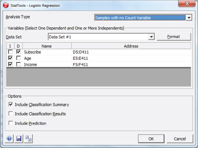
1. In StatTools use the Data Set Manager to select the range D4:F411.
2. From Regression and Classification select Logistic Regression....
3. Fill in the dialog box, as shown in Figure 17.13.
Figure 17-12: Logistic data with two independent variables
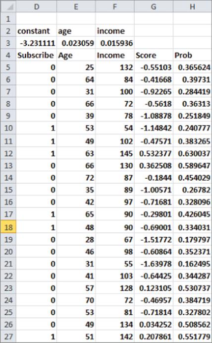
Figure 17-13: Variable selection for a Two Variable Logistic Model
You should obtain the output shown in Figure 17.14.
Figure 17-14: Output for Two Variable Logistic Regression
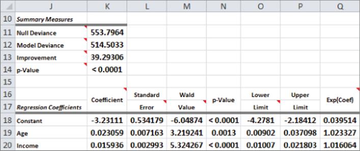
The p-value in K14 (< 0.0001) indicates that age and income together have less than 1 chance in 1,000 of not being helpful to predict whether a person is a subscriber. The small p-values in N19 and N20 indicate that each individual independent variable has a significant impact on predicting whether a person is a subscriber. Your estimate of the chance that a person is a subscriber is given by the following equation:
5 
In the cell range H5:H411, you use Equation 5 to compute the probability that a person is a subscriber. For example, from H6 you see the probability that a 64-year-old with an $84,000 annual income is a subscriber is 39.7 percent.
Performing a Logistic Regression with Count Data
In the previous section you performed logistic regression from data in which each data point was listed in an individual row. Sometimes raw data is given in a grouped, or count format. In count data each row represents multiple data points. For example, suppose you want to know how income (either low, medium, or high) and age (either young or old) influence the likelihood that a person purchases a product. Use the data from countdata2.xlsx, also shown in Figure 17.15. You can find, for example, that the data includes 500 young, low-income people, 35 of whom purchased your product.
Figure 17-15: Count data for logistic regression
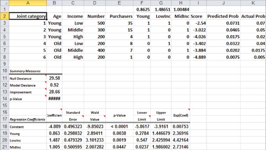
In F3:H8 IF statements are used to code age and income as dummy variables. The data omits old in the age variable and high in the income variable. For example, the range F8:H8 tells StatTools that row 8 represents old, high-income people.
To run a logistic regression with this count data, perform the following steps:
1. Use the Data Set Manager to select the range D2:H8.
2. Select Logistic Regression… from Regression and Classification, and fill in the dialog box, as shown in Figure 17.16. Note now the upper-left corner of the dialog box indicates that you told StatTools that count data was used.
Figure 17-16: Variable selection with count data
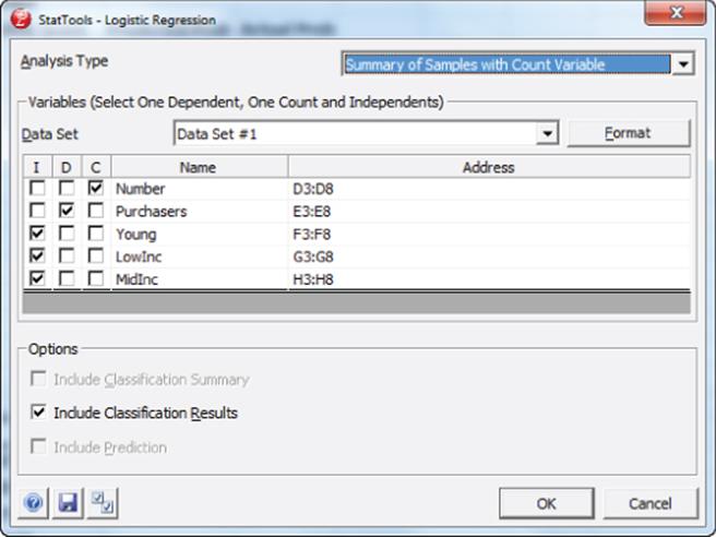
3. Select Number as the raw Count column and tell StatTools to predict purchasers using the Young, LowInc, and MidInc variables.
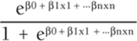
4. The p-values in E19:E21 indicate that each independent variable is a significant predictor of purchasing behavior. If you generalize Equation 4 you can predict in Column J the probability that a person would subscribe with the formula. Use the following equation to do so:

Refer to Figure 17.15 to see that the actual and predicted probabilities for each grouping are close.
Summary
In this chapter you learned the following:
· When the dependent variable is binary, the assumptions of multiple linear regression are violated.
· To predict the probability p that a binary-dependent variable equals 1, use the logit transformation:
1 ![]()
· The coefficients in Equation 1 are estimated using the method of Maximum Likelihood.
· You can use programs such as SAS, SPSS, and StatTools to easily estimate the logistic regression model and test the significance of the coefficients.
· Manipulation of Equation 1 shows the probability that a dependent variable equals one and is estimated by the following equation:
Exercises
1. For 1,022 NFL field goal attempts the file FGdata.xlsx contains the distance of the field goal and whether the field goal was good. How does the length of the field goal attempt affect the chance to make the field goal? Estimate the chance of making a 30, 40, or 50 yard field goal.
2. The file Logitsubscribedata.xls gives the number of people in each age group who subscribe and do not subscribe to a magazine. How does age influence the chance of subscribing to the magazine?
3. The file Healthcaredata.xlsx gives the age, party affiliation, and income of 300 people. You are also told whether they favor Obamacare. Develop a model to predict the chance that a person favors Obamacare. For each person generate a prediction of whether the person favors Obamacare. Interpret the coefficients of the independent variables in your logistic regression.
4. How would you incorporate nonlinearities and/or interactions in a logistic regression model?
5. The file RFMdata.xlsx contains the following data:
· Whether a person responded (dependent variable = 1) or did not respond (dependent variable = 0) to the most recent direct mail campaign.
· R: recency (time since last purchase) measured on a 1–5 scale; 5 indicates a recent purchase.
· F: frequency (how many orders placed in the last year) measured on a 1–5 scale with a 5 indicating many recent purchases.
· M: monetary value (total amount purchased in last year) measured on a 1–5 scale with a 5 indicating the person spent a lot of money in the last year on purchases.
Use this data to build a model to predict based on R, F, and M whether a person will respond to a mailing. What percentage of people responded to the most recent mailing? If you mailed to the top 10 percent (according to the logistic regression model) what response would be obtained?
6. Show that in a logistic regression model if an independent variable xi is increased by 1, then the odds ratio will increase by a factor of eβi.
7. Using the data in the data worksheet of the file subscribers.xlsx, show that for the magazine example logistic regression resolves the problems of non-normal residuals and heteroscedasticity.
8. The file shuttledata.xlsx contains the following data for several launches of the space shuttle:
· Temperature (degrees Fahrenheit)
· Number of O-rings on the shuttle and the number of O-rings that failed during the mission
Use logistic regression to determine how temperature affects the chance of an O-ring failure. The Challenger disaster was attributed to O-ring failure. The temperature at launch was 36 degrees. Does your analysis partially explain the Challenger disaster?
9. In 2012 the Obama campaign made extensive use of logistic regression. If you had been working for the Obama campaign how would you have used logistic regression to aid his re-election campaign?
All materials on the site are licensed Creative Commons Attribution-Sharealike 3.0 Unported CC BY-SA 3.0 & GNU Free Documentation License (GFDL)
If you are the copyright holder of any material contained on our site and intend to remove it, please contact our site administrator for approval.
© 2016-2026 All site design rights belong to S.Y.A.