Marketing Analytics: Data-Driven Techniques with Microsoft Excel (2014)

Part X. Marketing Research Tools

Chapter 38. Multidimensional Scaling (MDS)

Often a company wants to determine which industry brands are most similar and dissimilar to its own brand. To obtain this information a marketing analyst might ask potential customers to rate the similarity between different brands. Multidimensional scaling (MDS) enables you to transform similarity data into a one-, two-, or three-dimensional map, which preserves the ranking of the product similarities. From such a map a marketing analyst might find that, for example, Porsche and BMW are often rated as similar brands, whereas Porsche and Dodge are often rated as highly dissimilar brands. A chart generated by MDS in one or two dimensions can often be easily interpreted to tell you the one or two qualities that drive consumer preferences.

In this chapter you will learn how to collect similarity data and use multidimensional scaling to summarize product similarities in a one- or two-dimensional chart.

Similarity Data

Similarity data is simply data indicating how similar one item is to another item or how dissimilar one item is to another. This type of data is important in market research when introducing new products to ensure that the new item isn't too similar to something that already exists.

Suppose you work for a cereal company that wants to determine whether to introduce a new breakfast product. You don't know what product attributes drive consumer preferences. You might begin by asking potential customers to rank n existing breakfast products from most similar to least similar. For example, Post Bran Flakes and All Bran would be more similar than All Bran and Corn Pops. Because there are n(n-1)/2 ways to choose 2 products out of n, the product similarity rankings can range from 1 to n(n-1)/2. For example, if there are 10 products, the similarity rankings can range between 1 and 45 with a similarity ranking of 1 for the most similar products and a similarity ranking of 45 for the least similar products.

Similarity data is ordinal data and not interval data. Ordinal data is numerical data where the only use of the data is to provide a ranking. You have no way of knowing from similarities whether there is more difference between the products ranked 1 and 2 on similarity than the products ranked second and third, and so on. If the similarities are measured as interval data, the number associated with a pair of products reflects not only the ranking of the similarities, but also the magnitude of the differences in similarities. The discussion of MDS in this chapter will be limited to ordinal data. MDS based on ordinal data is known as nonmetric MDS.

MDS Analysis of U.S. City Distances

The idea behind MDS is to place products in a low (usually two) dimensional space so that products that are close together in this low-dimensional space correspond to the most similar products, and products that are furthest apart in the low-dimensional space correspond to the least similar products. MDS uses the Evolutionary Solver to locate the products under consideration in two dimensions in a way that is consistent with the product's similarity rankings. To exemplify this, you can apply MDS data to a data set based on the distances between 29 U.S. cities.

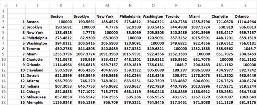
In the matrixnba worksheet of the distancemds.xls workbook you are given the distances between 29 U.S. cities based on the location of their NBA arenas (as shown in Figure 38.1). For reasons that will soon become clear the distance between a city and itself is set to be larger than any of the actual distances (for example, 100,000 miles). After ranking the distances between the cities (Brooklyn to New York is the shortest distance and Portland to Miami is the largest distance) you can locate each city in a two-dimensional space in a manner such that when the distances between each pair of cities in the two-dimensional space are ranked from smallest to largest, the ranks match, as closely as possible, to the rankings of the actual distances. Thus you would hope that in the two-dimensional space Brooklyn and New York would also be the closest pair of cities and Portland and Miami would be further apart than any other pair of cities. Before describing the process used to obtain the two-dimensional representation of the 29 cities, consider the OFFSET function, which is used in the approach to MDS.

Figure 38-1: Distances between U.S. cities

OFFSET Function

The syntax of the OFFSET function is OFFSET(cellreference, rowsmoved, columnsmoved, height, width). Then the OFFSET function begins in the cell reference and moves the current location up or down based on rows moved. (rowsmoved = –2, for example, means move up 2 rows and rowsmoved = +3 means move down three rows.) Then, based on columns moved, the current location moves left or right (for example, columnsmoved = –2 means move 2 columns to the left and rowsmoved =+3 means move 3 columns to the right). The current cell location is now considered to be the upper-left corner of an array with number of rows = height and number of columns = width.

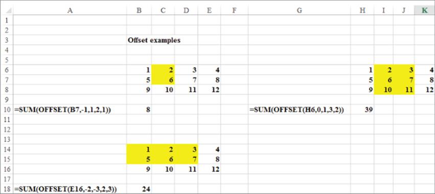
Figure 38.2 (see the Offsetexample. xls file) illustrates the use of the OFFSET function. For example, the formula =SUM(OFFSET(B7,-1,1,2,1)) begins in B7 and moves the cell location B7 one row up to B6. From B6 the cell location moves one column to the right to cell C6. Cell C6 now becomes the upper-left corner of a cell range with 2 rows and 1 column. The cells in this range (C6:C7) add up to 8. You should verify that the formulas in B18 and H10 yield the results 24 and 39, respectively.

Figure 38-2: Examples of OFFSET function

Setting up the MDS for Distances Data

The goal of MDS in the distances example is to determine the location of the cities in the two-dimensional space that best replicates the “similarities” of the cities. You begin by transforming the distances between the cities into similarity rankings so small similarity rankings correspond to close cities and large similarity rankings correspond to distant cities. Then the Evolutionary Solver is used to locate each city in two-dimensional space so that the rankings of the city distances in two dimensional space closely match the similarity rankings.

To perform the MDS on the distances data, proceed as follows:

1. In the range G3:H31 enter trial values for the x and y coordinates of each city in two-dimensional space. Arbitrarily restrict each city's x and y coordinate to be between 0 and 10.

2. Copy the formula =RANK(K3,distances,1) from K34 to the range K34:AM62 to compute the ranking of the distances between each pair of cities (see Figure 38.3). The last argument of 1 in this formula ensures that the smallest distance (New York to Brooklyn) receives a rank of 1, and so on. All diagonal entries in the RANK matrix contain 813 because you assigned a large distance to diagonal entries.

3. Copy the formula =IF($I66=K$64,10000000,(OFFSET($G$2,$I66,0,1,1)-OFFSET($G$2,K$64,0,1,1))^2+(OFFSET($H$2,$I66,0,1,1)-OFFSET($H$2,K$64,0,1,1))^2) from K66 to the range K66:AM94 to compute for each pair of different cities the square of the two-dimensional distances between each pair of cities. The term OFFSET($G$2,$I66,0,1,1) in the formula pulls the x coordinate of the city in the current row; the term OFFSET($G$2,K$64,0,1,1) pulls the x coordinate of the city in the current column; the term OFFSET($G$2,$I66,0,1,1) in the formula pulls the ycoordinate of the city in the current row; and the term OFFSET($H$2,K$64,0,1,1) pulls the y coordinate of the city in the current column. For distances corresponding to the same city twice, assign a huge distance (say 10 million miles). A subset of the distances in two-dimensional space is shown in Figure 38.4.

4. Your strategy is to have Solver choose the two-dimensional locations of the cities so that the ranking of the distances in the two-dimensional space closely matches the actual rankings of the distances. To accomplish this goal compute the ranking of the distances in two-dimensional space. Copy the formula (see Figure 38.5) =RANK(K66,twoddistances,1) from K98 to K98:AM126 to compute the rankings of the distances in two-dimensional space. For example, for the two-dimensional locations in G3:H31, Brooklyn and New York are the closest pair of cities.

5. In cell C3 compute the correlation between the original similarity ranks and the two-dimensional ranks with the formula =CORREL(originalranks,twodranks). The range K34:AM62 is named originalranks and the range K98:AM126 is named twodranks.

6. Use the Evolutionary Solver to locate each city in two-dimensional space to maximize the correlation between the original ranks and the ranks in two dimensions. This should ensure that cities that are actually close together will be close in two-dimensional space. Your Solver window is shown in Figure 38.6.

Figure 38-3: Ranking of distances between U.S. cities

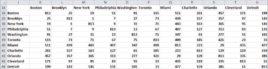
Figure 38-4: Two-dimensional distance between U.S. cities

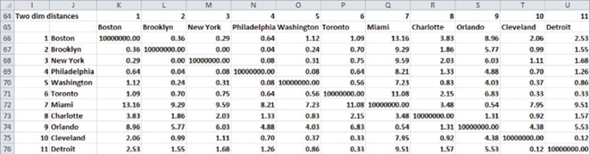
Figure 38-5: Ranking of two-dimensional distance between U.S. cities

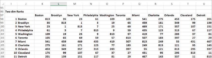
Figure 38-6: MDS Solver window cities

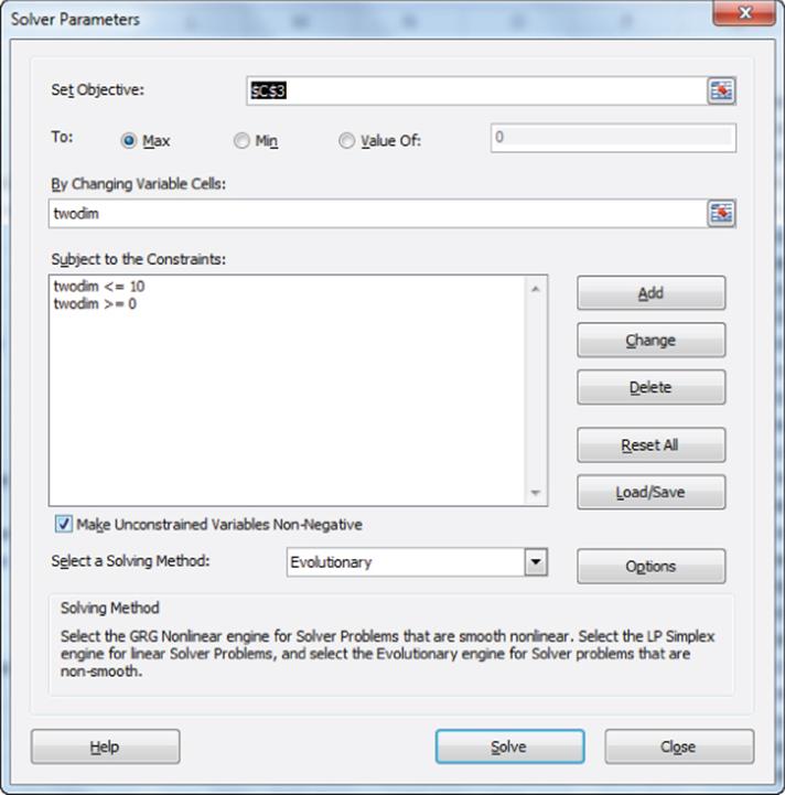
The Solver chooses for each city an x and y coordinate (changing cell range into two dimensions is the range G3:H31) to maximize the correlation between the original similarities and the two-dimensional distance ranks. You can arbitrarily constrain the x and y coordinates for each city to be between 0 and 10. The locations of each city in two-dimensional space are shown in Figure 38.7.

Figure 38-7: MDS Solver window cities

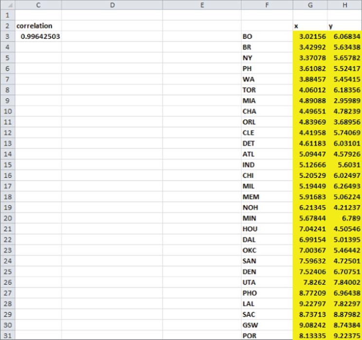
Referring to cell C3 of Figure 38.7, you can see that the correlation between the original similarity ranks and the two-dimensional ranks is an amazingly large 0.9964. Figure 38.8 shows a plot of the city locations in two-dimensional space.

Figure 38-8: Two-dimensional city plot

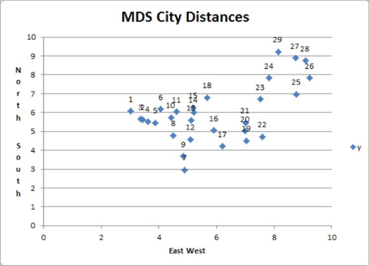
The cities on the right side of the chart are West Coast cities and the cities on the left side of the chart are East Coast cities. Therefore, the horizontal axis can be interpreted as an East West factor. The cities on the top of the chart are northern cities, and the cities on the bottom of the chart are southern cities. Therefore, the vertical axis can be interpreted as a North South factor. This example shows how MDS can visually demonstrate the factors that determine the similarities and differences between cities or products. In the current example distances are replicated via the two obvious factors of east-west (longitude) and north-south (latitude) distances. In the next section you will identify the two factors that explain consumer preferences for breakfast foods. Unlike the distances example, the two key factors that distinguish breakfast foods will not be obvious, and MDS will help you derive the two factors that distinguish breakfast foods.

MDS Analysis of Breakfast Foods

Paul Green and Vithala Rao (Applied Multidimensional Scaling, Holt, Rinehart and Winston, 1972) wanted to determine the attributes that drive consumer's preferences for breakfast foods. Green and Rao chose the 10 breakfast foods shown on the MDS worksheet in the breakfast.xls workbook and asked 17 subjects to rate the similarities between each pair of breakfast foods with 1 = most similar and 45 = least similar. (There are 45 different ways to choose 2 foods out of 10.) The ranking of the average similarity is also shown (see Figure 38.9). A rank of 0 is entered when a breakfast food is compared to itself. This ensures that the comparison of a food to itself does not affect the Solver solution.

Figure 38-9: Breakfast food data

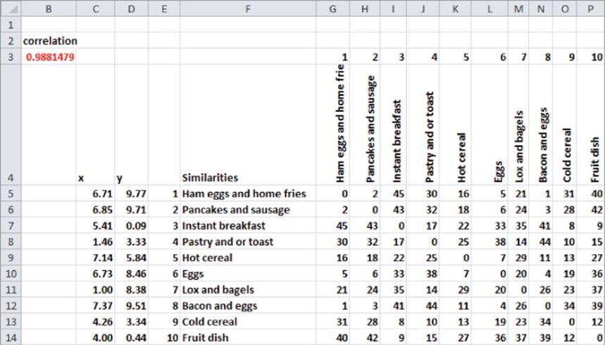
For example, the subjects on average deemed ham, eggs, and home fries and bacon and eggs as most similar and instant breakfast and ham, eggs, and home fries as least similar.

Using Card Sorting to Collect Similarity Data

Because of the vast range of the ranking scale in this scenario, many subjects would have difficulty ranking the similarities of pairs of 10 foods between 1 and 45. To ease the process the marketing analyst can put each pair of foods on 1 of 45 cards and then create four piles: highly similar, somewhat similar, somewhat dissimilar, and highly dissimilar. Then the subject is instructed to place each card into one of the four piles. Because there will be 11 or 12 cards in each pile, it is now easy to sort the cards in each pile from least similar to most similar. Then the sorted cards in the highly similar pile are placed on top, followed by the somewhat similar, somewhat dissimilar, and highly dissimilar piles. Of course, the card-sorting method could be easily programmed on a computer.

To reduce the breakfast food similarities to a two-dimensional representation, repeat the process used in the city distance example.

1. In the range C5:D14 (named location), enter trial values for the location of each food in two-dimensional space. As in the city distances example, constrain each location's x and y coordinate to be between 0 and 10.

2. Copy the formula =(INDEX(location,$E18,1)-INDEX(location,G$16,1))^2+(INDEX(location,$E18,2)-INDEX(location,G$16,2))^2 from G18 to G18:P27 (see Figure 38.10) to determine (given the trial x and y locations) the squared distance in two-dimensional space between each pair of foods. You could have used the OFFSET function to compute the squared distances, but here you choose to use the INDEX function. When copied down through row 27, the term INDEX(location,$E18,1), for example, pulls the x coordinate for the current row's breakfast food.

3. Copy the formula =IF(G$29=$E31,0,RANK(G18,$G$18:$P$27,1)) from G31 to G31:P40 to compute the rank (see Figure 38.11) in two-dimensional space of the distances between each pair of breakfast foods. For diagonal entries enter a 0 to match the diagonal entries in rows 5–14.

4. In cell B3 the formula =CORREL(similarities,ranks) computes the cor-relation between the average subject similarities and the two-dimensional distance ranks.

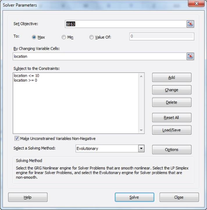
5. You can now use the Solver window shown in Figure 38.12 to locate the breakfast foods in two-dimensional space. The Solver chooses an x and y coordinate for each food that maximizes the correlation (computed in cell B3) between the subjects' average similarity rankings and the ranked distances in two-dimensional space. The Solver located the breakfast foods (refer to Figure 38.9). The maximum correlation was found to be 0.988.

Figure 38-10: Squared distances for breakfast foods example

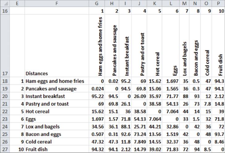
Figure 38-11: Two-dimensional distance ranks for breakfast food example

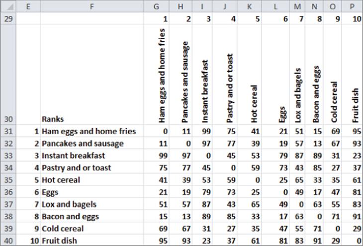
Figure 38-12: Solver window for breakfast food MDS

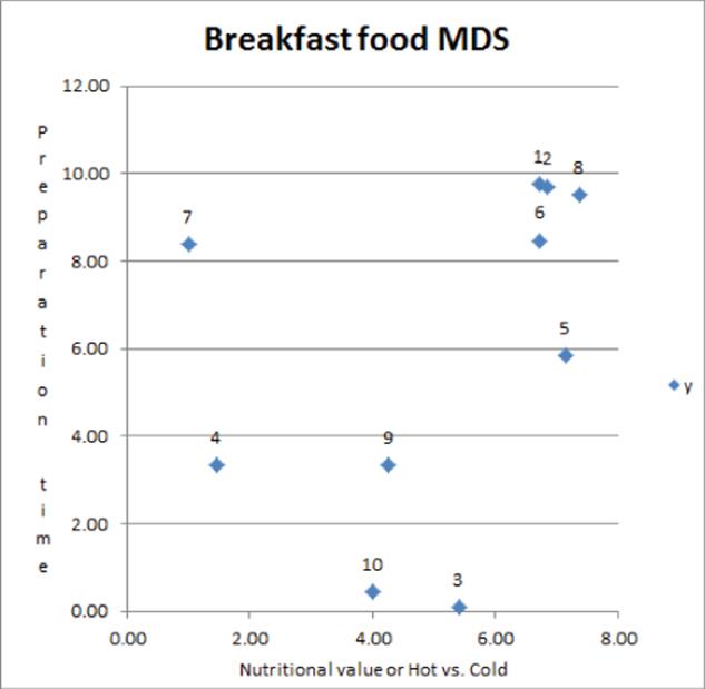
Unlike the previous MDS example pertaining to city distances, the labeling of the axis for the breakfast foods example is not as straightforward. This task requires taking a holistic view of the two-dimensional MDS map when labeling the axis. In this case, it appears that the breakfast foods on the right side of the chart tend to be hot foods and the foods on the left side of the chart tend to be cold foods (see the plot of the two-dimensional breakfast food locations in Figure 38.13). This suggests that the horizontal axis represents a hot versus cold factor that influences consumer preferences. The foods on the right also appear to have more nutrients than the foods on the left, so the horizontal axis could also be viewed as a nutritional value factor. The breakfast foods near the top of the chart require more preparation time than the foods near the bottom of the chart, so the vertical axis represents a preparation factor. The MDS analysis has greatly clarified the nature of the factors that impact consumer preferences.

Figure 38-13: Breakfast food MDS plot

Finding a Consumer's Ideal Point

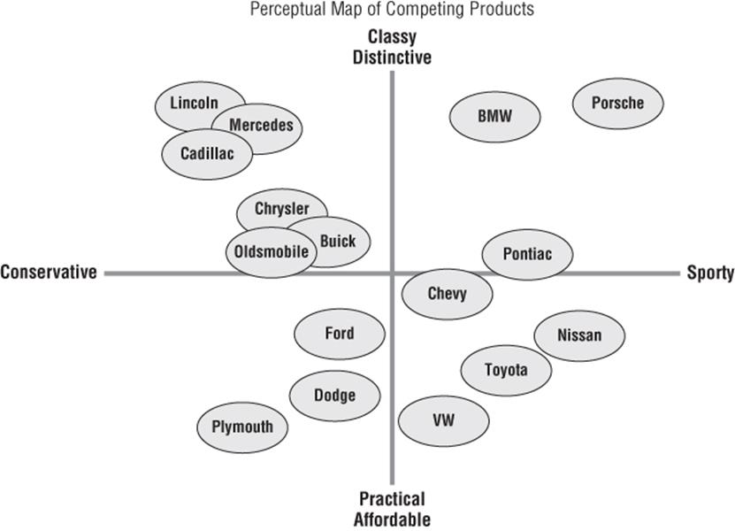
A chart that visually displays (usually in two dimensions) consumer preferences is called a perceptual map. A perceptual map enables the marketing analyst to determine how a product compares to the competition. For example, the perceptual map of automobile brands, as shown in Figure 38.14, is based on a sportiness versus conservative factor and a classy versus affordable factor. The perceptual map locates Porsche (accept no substitute!) in the upper-right corner (high on sportiness and high on classy) and the now defunct Plymouth brand in the lower-left corner (high on conservative and high on affordable).

Figure 38-14: Automobile brand perceptual map

When a perceptual map of products or brands is available, the marketing analyst can use an individual's ranking of products to find the individual's ideal point or most-wanted location on the perceptual map. To illustrate the idea I asked my lovely and talented wife Vivian to rank her preferences for the 10 breakfast foods (see Ideal Point worksheet of the breakfast.xls workbook and Figure 38.15). Vivian's product ranks are entered in the range D5:D14.

Figure 38-15: Finding the ideal point

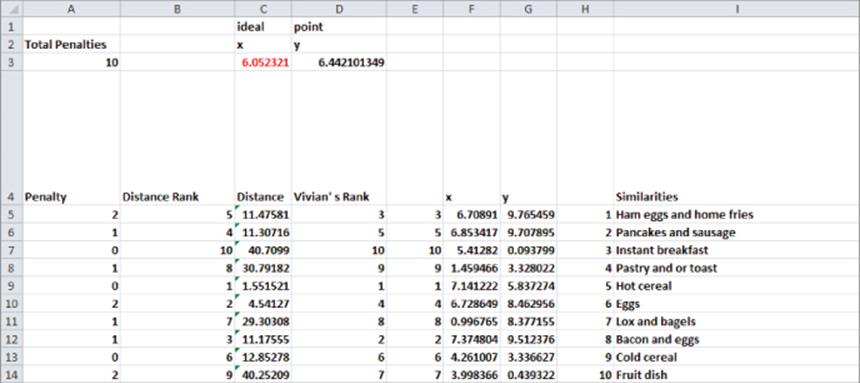
For example, Vivian ranked hot cereal first, bacon and eggs second, and so on. To find Vivian's ideal point, you can enter in the cell range C3:D3 trial values of x and y for the ideal point. To find an ideal point, observe that Vivian's highest ranked product should be closest to her ideal point; Vivian's second ranked product should be the second closest product to her ideal point; and so on. Now you will learn how Solver can choose a point that comes as close as possible to making less preferred products further from Vivian's ideal point. Proceed as follows:

1. Copy the formula =SUMXMY2($C$3:$D$3,F5:G5) from C5 to C6:C14 to compute the squared distance of each breakfast food from the trial ideal point values.

2. Copy the formula =RANK(C5,$C$5:$C$14,1) from B5 to B6:B14 to rank each product's squared distance from the ideal point.

3. Copy the formula =ABS(B5-D5) from A5 to A6:A14 to compute the difference between Vivian's product rank and the rank of the product's distance from the ideal point.

4. In cell A3 use the formula =SUM(A5:A14) to compute the sum of the deviations of Vivian's product ranks from the rank of the product's distance from the ideal point. Your goal should be to minimize this sum.

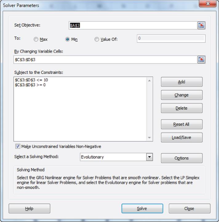
5. The Solver window, as shown in Figure 38.16, can find an ideal point (not necessarily unique) by selecting x and y values between 0 and 10 that minimize A3.

Figure 38-16: Solver window for finding the ideal point

As shown in Figure 38.17, Vivian's ideal point is x = 6.06 and y = 6.44, which is located between her two favorite foods: hot cereal and bacon and eggs. The sum of the deviation of the rankings of the product distances from the ideal point and the product rank was 10.

Figure 38-17: Vivian's ideal point

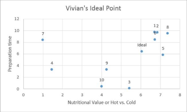
You can use ideal points to determine an opportunity for a new product. After plotting the ideal points for, say, 100 potential customers, you can use the techniques in Chapter 23, “Cluster Analysis,” to cluster customer preferences based on the location of their ideal points on the perceptual map. Then if there is a cluster of ideal points with no product close by, a new product opportunity exists. For example, suppose that there were no Diet 7UP or Diet Sprite in the market and an analysis of soft drink similarities found the perceptual map shown in Figure 38.18.

Figure 38-18: Soda perceptual map

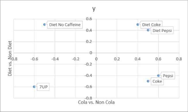
You can see the two factors are Cola versus non-Cola (x axis) and Diet versus non-Diet (y axis). Suppose there is a cluster of customer ideal points near the point labeled Diet no caffeine. Because there is currently no product near that point, this would indicate a market opportunity for a new diet soda containing no caffeine (for example Diet 7UP or Diet Sprite).

Summary

In this chapter you learned the following:

· Given product similarity you can use data nonmetric MDS to identify a few (usually at most three) qualities that drive consumer preferences.

· You can easily use the Evolutionary to locate products on a perceptual map.

· Use the Evolutionary Solver to determine each person's ideal point on the perceptual map. After clustering ideal points, an opportunity for a new product may emerge if no current product is near one of the cluster anchors.

Exercises

1. Forty people were asked to rank the similarities between six different types of sodas. The average similarity rankings are shown in Figure 38.19. Use this data to create a two-dimensional perceptual map for sodas.

Figure 38-19: Soda perceptual map

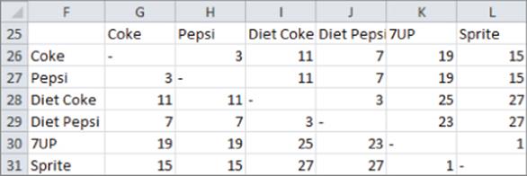
2. The ranking for the sodas in Exercise 1 is Diet Pepsi, Pepsi, Coke, 7UP, Sprite, and Diet Coke. Determine the ideal point.

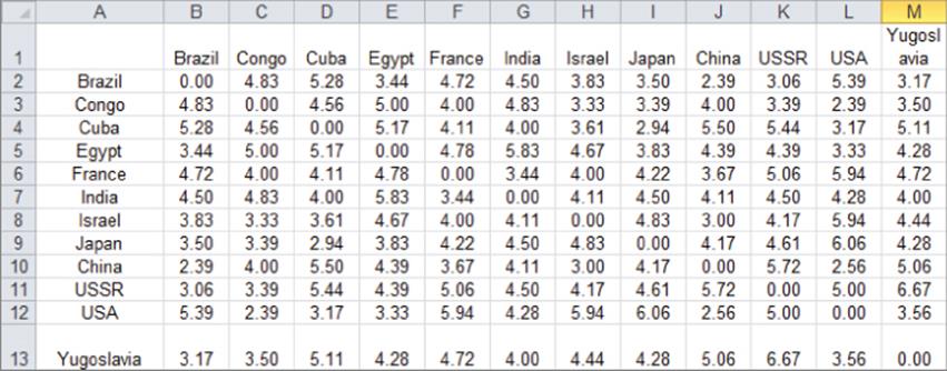
3. The file countries.xls (see Figure 38.20) gives the average ratings 18 students gave when asked to rank the similarity of 11 countries on a 9-point scale (9 = highly similar and 1 = highly dissimilar). For example, the United States was viewed as most similar to Japan and least similar to the Congo. Develop a two-dimensional perceptual map and interpret the two dimensions.

Figure 38-20: Exercise 3 data

4. Explain the similarities and differences between using cluster analysis and MDS to summarize multidimensional data.

5. Explain the similarity and differences between using principal components and MDS to summarize multidimensional data.