Marketing Analytics: Data-Driven Techniques with Microsoft Excel (2014)

Part X. Marketing Research Tools

Chapter 39. Classification Algorithms: Naive Bayes Classifier and Discriminant Analysis

In marketing and other areas, analysts often want to classify an object into one of several (most often two) groups based on knowledge of several independent variables, for example:

· Based on gender, age, income, and residential location, can you classify a consumer as a user or nonuser of a new breakfast cereal?

· Based on income, type of residence, credit card debts, and other information, can you classify a consumer as a good or bad credit risk?

· Based on financial ratios, can you classify a company as a likely or unlikely candidate for bankruptcy?

· Based on cholesterol levels, blood pressure, smoking, and so on, is a person at high risk for a heart attack?

· Based on GMAT score and undergraduate GPA, is an applicant a likely admit or reject to an MBA program?

· Based on demographic information, can you predict which car model a person will prefer?

In each of these situations, you want to use independent variables (often referred to as attributes) to classify an individual. In this chapter you learn two methods used for classification: Naive Bayes classifier and linear discriminant analysis.

You begin this chapter by studying some topics in basic probability theory (conditional probability and Bayes' Theorem) that are needed to understand the Naive Bayes classifier. Then you learn how to easily use the Naive Bayes classifier to classify observations based on any set of independent variables. Finally you learn how to use the Evolutionary Solver (first discussed in Chapter 5, “Price Bundling”) to develop a linear discriminant classification rule that minimizes the number of misclassified observations.

Conditional Probability

The concept of conditional probability essentially allows you to adjust the probability of an event (A) based on the occurrence of another event (B.) Therefore, given two events A and B, you write P(A|B) to denote the conditional probability that event A occurs, given you know that event B occurs. P(A|B) may be written as the following equation:

1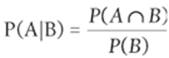

Equation 1 can be rearranged to yield Equation 2:

2

In Equation 1, denotes the probability that A and B occur. To illustrate the idea of conditional probability, suppose that 10 percent of all adults watch the TV show The Bachelor. Assume that 80 percent of The Bachelor viewers are women and that one-half of U.S. adults are men. Define the following as:

· B = Event adult watches “The Bachelor”

· M = Event adult is a man

· W = Event adult is a woman

· NB = Event adult does not watch “The Bachelor”

To illustrate the concept of conditional probability you will compute the probability that a given woman or man is a Bachelor viewer. Assume one-half of all adults are men. All adults fall into one of four categories: women Bachelor viewers, men Bachelor viewers, men non-Bachelor viewers, and women non-Bachelor viewers. Now calculate the fraction of all adults falling into each of these categories. Note that from Equation 2 you can deduce the following:

Because the first row of the Table 39.1 must add up to 0.10 and each column must add up to 0.5, you can readily compute all probabilities.

Table 39.1 Bachelor Probabilities

To cement your understanding of conditional probability, compute P(B|W) and P(B|M). Referring to Table 39.1 and Equation 1, you can find that:

In other words, 16 percent of all women and 4 percent of all men are Bachelor viewers. In the next section you learn how an extension of conditional probability known as Bayes' Theorem enables you to update conditional probabilities based on new information about the world.

Bayes' Theorem

Bayes' Theorem was developed during the 18th century by the English minister Thomas Bayes.

NOTE

If you are interested in exploring the fascinating history of Bayes' Theorem, read Sharon McGrayne's marvelous book The Theory That Would Not Die (Yale University Press, 2011).

To introduce Bayes' Theorem you can use a nonmarketing example commonly taught to future doctors in medical school. Women are often given mammograms to detect breast cancer. Now look at the health of a 40-year-old woman with no risk factors for breast cancer. Before receiving a mammogram, the woman's health may be classified into one of two states:

· C = Woman has breast cancer.

· NC = Woman does not have breast cancer.

Refer to C and NC as states of the world. A priori, or before receiving any information, it is known that P(C) = 0.004 and P(NC) = 0.996. These probabilities are known as prior probabilities. Now the woman undergoes a mammogram and one of two outcomes occurs:

· + = Positive test result

· – = Negative test result

Because many healthy 40-year-old women receive mammograms, the likelihood of a positive test result for a healthy 40-year-old woman or a 40-year-old woman with breast cancer is well known and is given by P(+|C) = 0.80 and P(+|NC) = 0.10.

The goal of Bayes' Theorem is to factor in observed information (in this case mammogram results) and update the prior probabilities to determine posterior probabilities that incorporate the mammogram test results. In this example, you need to determine P(C|+) and P(C|–).

Essentially, Bayes' Theorem enables you to use Equation 1 to factor in likelihoods and prior probabilities to compute posterior probabilities. For example, to compute P(C|+) use Equation 1 to find that:

3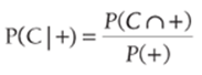

To compute the denominator of Equation 3, observe that a + test result can be observed from women with cancer and women without cancer. This implies that P(+) = . Then by Equation 2 you find P(+) = P(+|C) * P(C) + P(+|NC) * P(NC). Substituting this result in the denominator of Equation 3 yields the following:

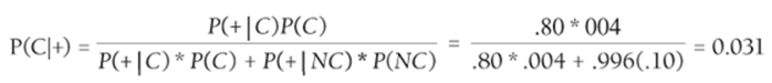
Thus even after observing a positive mammogram result, there is a small chance that a healthy 40-year-old woman has cancer. When doctors are asked to determine P(C|+) for the given data, only 15 percent of the doctors get the right answer (see W. Casscells, A. Schoenberger, and T.B. Graboys, “Interpretation by physicians of clinical laboratory results,” New England Journal of Medicine, 1978, pp. 999–1001)!

Here is a more intuitive way to see that P(C|+) = 0.031: Look at 10,000 women and determine how many of them fall into each possible category (Cancer and +, Cancer and –, No Cancer and +, No Cancer and –).

· 10,000(0.004) = 40 women have cancer.

· Because P(+|C) = 0.8, 80 percent of the 10,000 women, or 32 women, will have cancer and test positive.

· 10,000(0.996) = 9,960 women do not have cancer.

· Since P(+|NC) = 0.10, 9,960 * (0.10) = 996 women without cancer test positive!

· Combining your knowledge that 32 women with cancer test positive and 996 women without cancer test positive with the fact that the first row of Table 39.2 must total to 40 and the second row totals to 9,960, you may complete Table 39.2.

Table 39.2 Another Way to Understand Bayes' Theorem

Now it is clear that P(C|+) = 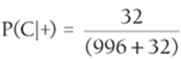= 0.031.

This argument makes it apparent that the large number of false positives is the reason that the posterior probability of cancer after a positive test result is surprisingly small. In the next section you use your knowledge of Bayes' Theorem to develop a simple yet powerful classification algorithm.

Naive Bayes Classifier

The general classification problem may be stated as follows: Each observation is in one of k classes: C₁, C, … C_k, but for each observation you do not know to which class the observation belongs. For each observation you know the values of n attributes X₁, X₂ , …., X_n. In this discussion of Naive Bayes, assume each attribute is a qualitative variable (such as a person is male or female) and not quantitative (such as a person's height or weight). Given knowledge of the attributes, to which class should you assign an observation? To explain how the Naive Bayes classifier works, assumen = k = 2. Then it seems reasonable to compute P(C₁|X₁, X₂) and P(C₂|X₁, X₂) and classify the object in the class with the larger posterior probability. Before showing how Naive Bayes is used to compute these probabilities, you need to develop Equation 4 to compute joint probabilities involving attributes and categories.

4

Applying Equation 1 twice to the right side of Equation 4 transforms the right side of Equation 4 to , which is the left side of Equation 3. This proves the validity of Equation 4. Now applying Equation 1 and Equation 4 you can show that

5

NOTE

The key to Naive Bayes is to assume that in computing you may assume that this probability is conditionally independent of (does not depend on) X₁. In other words, may be estimated as P(X₂|C₁). Because this assumption ignores the dependence between attributes, it is a bit naive; hence the name Naive Bayes.

Then, using Equation 5, the posterior probability for each class may be estimated with Equations 6 and 7.

6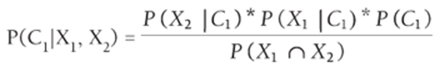

7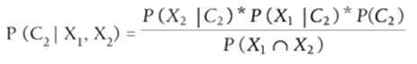

Because the posterior probabilities of all the classes should add to 1, you can compute the numerators in Equations 6 and 7 and normalize them so they add to 1. This means that you can ignore the denominators of Equation 6 and 39.7 in computing the posterior probabilities. Then an observation is assigned to the class having the largest posterior probability.

More generally, if you have knowledge of n attributes, Naive Bayes estimates the posterior probability of class C_i by using Equation 8:

8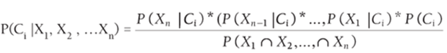

The numerator of Equation 8 can easily be computed for each class from sample data using COUNTIFS functions. Then each observation is assigned to the class having the largest posterior probability. You might ask why not just use COUNTIFS functions to exactly compute the numerator ofEquation 8 by estimating P(X₁∩X₂,…,∩X_n∩C_i) as the fraction of all observations that are in class C_i and have the wanted attribute values. The problem with this approach is that if there are many attributes there may be few or no observations in the relevant class with the given attribute values. Because each P(X_k|C_i) is likely to be based on many observations, the Naive Bayes classifier avoids this issue.

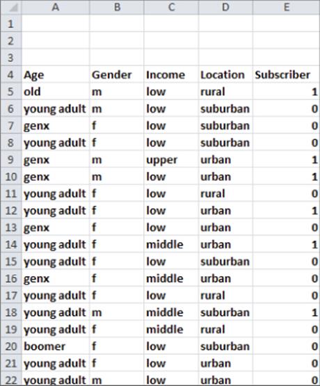
You are now ready to apply the Naive Bayes classifier to an actual example. The file ESPNBayes.xlsx (see Figure 39.1) contains the following information for a random sample of U.S. adults:

· Age: Young Adult, Gen X, Boomer, or Old

· Gender: Male (M) or Female (F)

· Income: Low, Middle, or Upper

· Location: Rural, Suburban, or Urban

· Whether the person is a subscriber (39.1) or a nonsubscriber (0)

Figure 39-1: ESPN Naive Bayes classifier data

Your goal is to compute the posterior probability that a person is a subscriber or nonsubscriber given the person's age, gender, income, and location. As shown in Figure 39.2, you need to compute the following quantities:

· For each attribute the likelihood of the attribute is conditioned on whether the person is a subscriber or nonsubscriber. For example, for gender you need to compute P(M|S), P(F|S), P(M|NS), and P(M|NS).

· For a subscriber and nonsubscriber, compute (given the person's value for each attribute) the numerator of Equation 8 by multiplying the class (either N or NS) prior probability times the conditional probability of each attribute value based on the class value.

· Normalize the numerator of Equation 8 for each class, so the posterior probabilities add to 1.

Figure 39-2: GenX, middle income, urban, male is classified as subscriber.

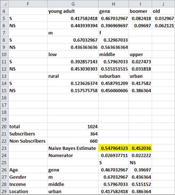
These calculations proceed as follows:

1. In cell G21 compute the number of subscribers (364) with the formula =COUNTIF(E5:E1030,1).

2. In cell G22 compute the number of nonsubscribers (660) with the formula =COUNTIF(E5:E1030,0).

3. In cell G20 compute the total number of subscribers (1,024) with the formula =SUM(G21:G22).

4. Copy the formula =COUNTIFS($A$5:$A$1030,G$4,$E$5:$E$1030,1)/$G21 from G5 to G5:J6 to compute for each class age combination the conditional probability of the age given the class. For example, cell H5 tells you that P(GenX|S) = 0.467.

5. Copy from G8 to G8:H9 the formula =COUNTIFS($B$5:$B$1030,G$7,$E$5:$E$1030,1)/$G21 to compute for each class gender combination the conditional probability of the gender given the class. For example, the formula in cell H9 tells you that P(F|NS) = 0.564.

6. Copy the formula =COUNTIFS($C$5:$C$1030,G$10,$E$5:$E$1030,1)/$G21 from G11 to G11:I12 to compute for each class income combination the conditional probability of the income given the class. For example, the formula in cell I11 tells you P(Middle|S) = 0.580.

7. Copy the formula =COUNTIFS($D$5:$D$1030,G$13,$E$5:$E$1030,1)/$G21 from G14 to G14:I15 to compute for each class location combination the conditional probability of the location given the class. For example, the formula in cell G14 tells you P(Rural|S) = 0.124.

8. In the cell range G26:G29, use a drop-down box to select the level of each attribute. For example, with the cursor in cell G26, the drop-down box was created by selecting Data Validation from the Data tab and filling in the dialog box, as shown in Figure 39.3.

9. Copy the formula =HLOOKUP($G26,INDIRECT($F26),2,FALSE) from H26 to H26:H29 to look up the conditional probability of each of the person's attributes given that the person is a subscriber. For example, in H27 you can find that 67 percent of all subscribers are male. Note the lookup ranges for each attribute are named as age, gender, income, and location, respectively. Combining these range name definitions with the INDIRECT function enables you to easily reference the lookup range for each attribute based on the attribute's name!

10. Copy the formula =HLOOKUP($G26,INDIRECT($F26),3,FALSE) from I26 to I26:I29 to look up the conditional probability of each of the person's attributes given that the person is not a subscriber. For example, in I27 you can find that 44 percent of the nonsubscribers are male.

11. In H24 the formula =PRODUCT(H26:H29) * Non Subscribers/total computes the numerator of Equation 8 for the classification of the person as a subscriber. The PRODUCT term in this formula multiplies the conditional likelihood of each attribute based on the assumption that the person is a subscriber, and the Subscribers/Total portion of the formula estimates the probability that a person is a subscriber.

12. In I24 formula =PRODUCT(I26:I29)*Subscribers/total computes the numerator of Equation 8 for the classification of the person as a nonsubscriber.

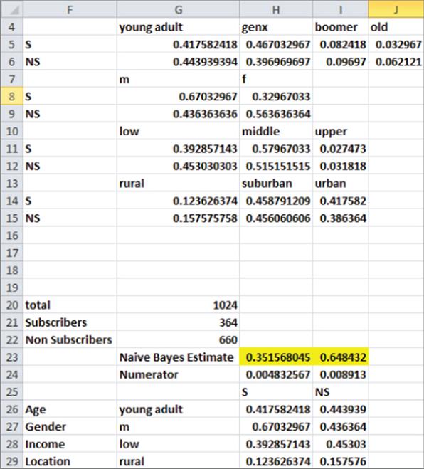
13. Copy the formula =H24/SUM($H24:$I24) from H23 to I23 to normalize the numerators for Equation 8 so the sum of the posterior probabilities add to 1. You can find that for a middle income, urban, Gen X male Naive Bayes estimates a 54.8 percent chance the person is a subscriber and a 45.2 percent chance that the person is not a subscriber. Because Naive Bayes gives a higher probability that the person is a subscriber than a nonsubscriber, you would classify the person as a subscriber. As shown in Figure 39.4, a low income, rural, young adult male would be estimated to have only a 35.2 percent chance of being a subscriber and would be classified as a nonsubscriber.

Figure 39-3: Creating a drop-down list for age

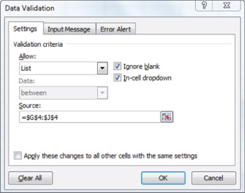
Figure 39-4: Young adult, low income, rural male is classified as nonsubscriber

The Naive Bayes classifier has been successfully applied to many classification problems including:

· Classifying e-mails as spam or nonspam based on words contained in the email

· Classifying a person as likely to develop Alzheimer's disease based on the genome makeup

· Classifying an airline flight as likely to be on time or delayed based on the airline, airport, weather conditions, time of day, and day of week

· Classifying customers as likely or unlikely to return purchases based on demographic information

Similarly, for a more in-depth example, Naive Bayes can be used to efficiently allocate marketing resources. Suppose ESPN The Magazine is trying to determine how to allocate its TV advertising budget. For each TV show Nielson can provide ESPN with the demographic makeup of the show's viewing population. Then Naive Bayes can be used to estimate the number of subscribers among the show's viewers. Finally, the attractiveness of the shows to ESPN could be ranked by Estimated Subscribers in Viewing Population/Cost per Ad.

Linear Discriminant Analysis

Similar to Naive Bayes classification, linear discriminant analysis can be used in marketing to classify an object into a group based on certain features. However, whereas Naive Bayes classifies objects based on any given independent variable, linear discriminant analysis uses a weighted, linear combination of variables as the basis for classification of each observation.

In the discussion of linear discriminant analysis you can assume that n continuous valued attributes X₁ , X₂, …, X_n are used to classify an observation into 1 of 2 groups. A linear classification rule is defined by a set of weights W₁, W₂, … W_n for each attribute and a cutoff point Cut. Each observation is classified in Group 1 if the following is true:

The observation is classified in Group 2 if the following is true:

You can call W1(value of variable 1) + W2(value of variable 2) + …Wn(value of variable n) the individual's discriminant score.

The goal is to choose the weights and cutoff to minimize the number of incorrectly classified observations. The following examples show how easy it is to use the Evolutionary Solver to find an optimal linear classification rule.

Finding the Optimal Linear Classification Rule

The file WSJ.xlsx (see Figure 39.5) contains the annual income and size of investment portfolio (both in thousands of dollars) for 84 people. A “0” indicates the person does not subscribe to The Wall Street Journal, whereas a “1” indicates the person is a subscriber. Using income and size of investment portfolio, you can determine a linear classification rule that minimizes the number of people incorrectly classified as subscribers or nonsubscribers by following these steps:

1. In F3:G3 enter trial values for the income and investment weights. In H3 enter a trial value for the cutoff.

2. In F5:F88 compute each individual's “score” by copying from F5 to F6:F88 the formula =SUMPRODUCT($F$3:$G$3,C5:D5).

3. In G5:G88 compare each person's score to the cutoff. If the score is at least equal to the cutoff, classify the person as a subscriber. Otherwise, classify the person as a nonsubscriber. To accomplish this goal copy the formula =IF(F5>$H$3,1,0) from G5 to G6:G88.

4. In H5:H88 determine if you correctly or incorrectly classified the individual. A “0” indicates a correct classification, whereas a “1” indicates an incorrect classification. Simply copy the formula =IF(G5-E5=0,0,1) from H5 to H6:H88.

5. In I5 use the formula =SUM(H5:H88) to compute the total number of misclassifications by adding up the numbers in Column H.

6. Because your spreadsheet involves many non-smooth functions (IF statements) use the Evolutionary Solver to devise a classification rule that minimizes the number of errors. The Solver window, as shown in Figure 39.6, chooses the weights and cutoffs to minimize the number of errors.

Figure 39-5: Wall Street Journal subscriber data

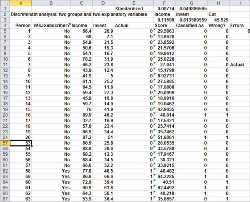
Figure 39-6: Solver window for Wall Street Journal example

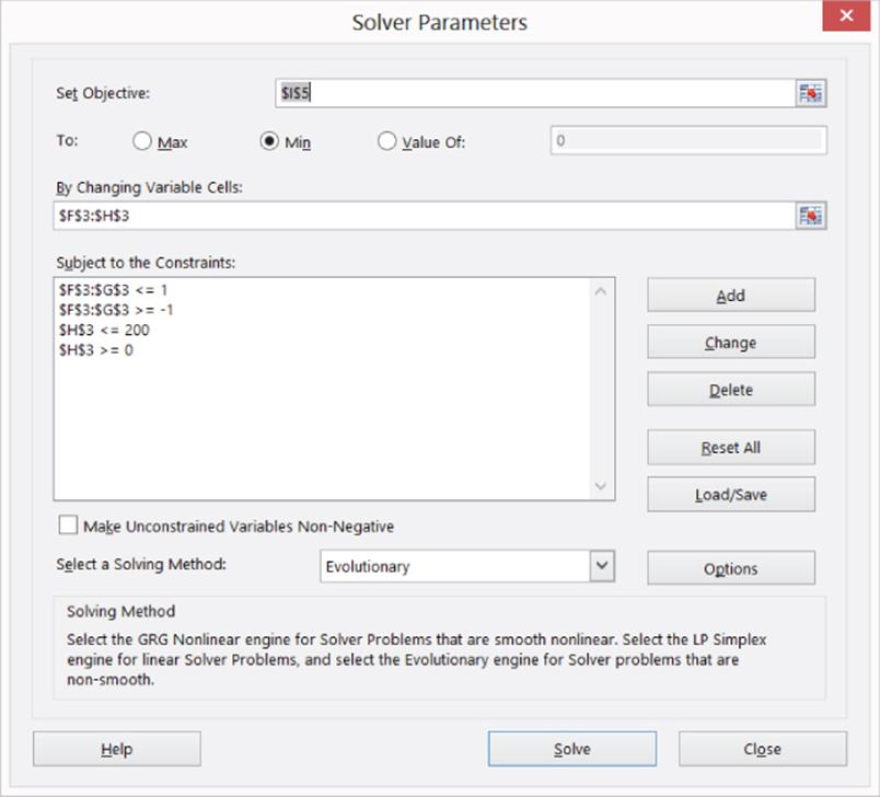
You want to minimize the total number of misclassifications (cell I5) by adjusting weights (F3 and G3) and the cutoff (H3). Recall that to use the Evolutionary Solver weights are needed on the changing cells. It is not clear what bounds to place on the changing cells. Because the cutoff may be set to any number, the keys to the classification are the ratios of the attribute weights. Without loss of generality you can assume an upper bound of 1 on each weight and a lower bound of –1). For example, if Solver found that a person should be classified as a subscriber if 2 * (Income) + 5(Investment Portfolio) >= 200, then you could simply divide the rule by 5 and rewrite the rule as 0.4 * (Income) + Investment Portfolio >= 40.

This equivalent classification rule has weights that are between –1 and +1. After noting that the maximum income is 100.7 and the maximum investment portfolio is 66.6, you can see that the maximum score for an individual would be 1 * (100.7) + 1 * (66.6) = 167.3. To be conservative, the upper bound on the cutoff was set to 200. The Evolutionary Solver was used because the model has many IF statements. After setting the Mutation rate to 0.5, the Solver found the following classification rule: If 0.116 * (Income in 000's) + 0.814 * (Investment amount in 000's) ≥ 45.529, then classify the individual as a subscriber; otherwise classify the individual as a nonsubscriber. Only 6 or 7.1 percent of the individuals are incorrectly classified. There are many different classification rules that yield six errors, so the optimal classification rule is not unique.

Finding the Most Important Attributes

You might think that the attribute with the largest weight would be most important for classification. The problem with this idea is that the weights are unit-dependent. For example, if the investment portfolio were measured in dollars, the weight for the Investment Portfolio would be 0.814/1,000, which would be much smaller than the income weight. The attributes may be ranked, however, if the weight for each attribute is standardized by dividing by the standard deviation of the attribute values. These standardized weights are computed in the cell range F1:G1 by copying from F1 to G1 the formula =F3/STDEV(C5:C88). Because the standardized investment portfolio weight is much larger than the standardized income weight, you can conclude, if you want to classify a person as a subscriber or nonsubscriber to the Wall Street Journal, that an individual's investment portfolio is more useful than the individual's annual income.

Classification Matrix

The results of a linear discriminant analysis are often summarized with a classification matrix, which gives for each class the number of observations that are correctly and incorrectly classified. The classification matrix for the Wall Street Journal example is shown in Figure 39.7.

Figure 39-7: Classification matrix for Wall Street Journal example

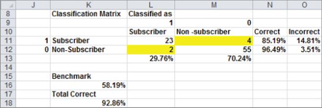
You can compute the classification matrix by copying the formula =COUNTIFS(Actual,$J11,Classified,L$9) from L11 to L11:M12. The range name Actual refers to E5:E88 and the range name Classified refers to G5:G88. For each class the percentage of observations classified correctly and incorrectly is computed in the range N11:O12. Therefore, 85.19 percent of all subscribers are classified correctly, and 96.49 percent of nonsubscribers are classified correctly.

Evaluating the Quality of the Classification Rule

In the WSJ example 79 / 85 = 92.86 percent of all observations were correctly classified. To evaluate the performance of the linear classification rule, you can develop a benchmark classification rate. Suppose fraction P_i of the observations are members of class i. Then a simple classification procedure (known as proportional classification) would be to randomly classify each observation in class 1 with probability P₁ and randomly classify each observation in class 2 with probability P₂. Using proportional classification, the fraction of observations correctly classified can be computed as

In the Wall Street Journal example proportional classification would classify (0.2976)² + (0.7024)² = 58.19 percent.

The 92.86 percent correct classification rate looks good when compared to the 58.19 percent benchmark as set via proportional classification.

Linear Classification with More Than Two Groups

You can easily use the Evolutionary Solver to determine an optimal linear classification rule when there are more than two groups. To illustrate the idea suppose you want to classify MBA applicants as likely admits, likely rejects, or marginal admits based on the applicants' GMAT scores and undergraduate GPAs. As changing cells you can use W₁ and W₂ as weights and use two cutoffs: C₁ and C₂. Then the classification rule works as follows:

· Classify applicant as likely admit if W₁ * GMAT + W₂ * GPA >= C₁

· Classify applicant as marginal admit if C₁ > W₁ * GMAT + W₂ * GPA > C₂

· Classify applicant as likely reject if W₁ * GMAT + W₂ * GPA <= C₂

You can use the Evolutionary Solver to choose the values of W₁, W₂, C₁, and C₂ that minimize the number of classification errors.

Classification Rules Involving Nonlinearities and Interactions

A classification rule involving nonlinearities and interactions could significantly improve classification performance. The Wall Street Journal example illustrates how you can evaluate a classification rule involving nonlinearities. Following the discussion of nonlinearities and interactions in Chapter 10, “Using Multiple Regression to Forecast Sales,” you would choose C, W₁, W₂, W₃, W₄, and W₅ so that the following classification rule minimizes classification errors.

If W₁*(Income) + W₂(Investment Portfolio) +W₃(Income²) + W₄*(Investment Portfolio² ) + W₅*(Income*Investment Portfolio)>=C, then classify the person as a subscriber; otherwise classify the person as a nonsubscriber. This classification rule (see Exercise 4) improves the number of errors from 6 to 5. This small improvement indicates that you are justified in using the simpler linear classification rule instead of the more complex rule involving nonlinearities and interactions.

Model Validation

In practice, classification models such as Naive Bayes and linear discriminant analysis are deployed using a “calibration” and “validation” stage. The model is calibrated using approximately 80 percent of the data and then validated using the remaining 20 percent of the data. This process enables the analyst to determine how well the model will perform on unseen data. For example, in the Wall Street Journal example suppose in the testing phase 95 percent of observations were correctly classified but in the validation phase only 75 percent of the observations were correctly classified. The relatively poor performance of the classification rule in the validation phase would make you hesitant to use the rule to classify new observations.

The Surprising Virtues of Naive Bayes

In addition to linear discriminant analysis, logistic regression (see Chapter 17, “Logistic Regression”) and neural networks (see Chapter 15, “Using Neural Networks to Forecast Sales”) can be used for classification. All these methods utilize sophisticated optimization techniques. On the other hand, Naive Bayes uses only high school probability and simple arithmetic for classification. Despite this fact, Naive Bayes often outperforms the other sophisticated classification algorithms (see D.J. Hand and K. Yu, “Idiot's Bayes — not so stupid after all?” International Statistical Review, 2001, pp. 385–99.) The surprising performance of Naive Bayes may be because dependencies between attributes are often distributed evenly between classes or dependencies between attributes can cancel each other out when used for classification. Finally, note the following two advantages of Naive Bayes:

· If you have made your data an Excel table, then when new data is added, your Naive Bayes analysis automatically updates while other classification rules require you to rerun a neural network, logistic regression, or linear discriminant analysis.

· If an important attribute is missing from the analysis this can greatly reduce the performance of a classification analysis based on a neural network, logistic regression, or linear discriminant analysis. The absence of an important attribute will often have little effect on the performance of a Naive Bayes classification rule.

Summary

In this chapter you learned the following:

· In the general classification problem, you classify an observation into 1 of k classes based on knowledge of n attributes.

· Given values X₁, X₂, …., X_n for the attributes, the Naive Bayes classifier classifies the observation in the class that maximizes

· A linear classification rule for two classes is defined by weights for each attribute and a classification cutoff. Each observation is classified in class 1 if the following is true:

It is classified in class 2 otherwise.

· You can use the Evolutionary Solver to determine the weights and cutoffs that minimize classification errors.

Exercises

1. For 49 U.S. cities, the file Incomediscriminant.xlsx contains the following data:

· Income level: low, medium, or high

· Percentage of blacks, Hispanics, and Asians

(a) Use this data to build a linear classification rule for classifying a city as low, medium, or high income.

(b) Determine the classification matrix.

(c) Compare the performance of your classification rule to the proportional classification rule.

2. For a number of flights, the file Flighttimedata.xlsx contains the following information:

· Was the flight on time or delayed?

· Day of week: 1 = Monday, 2 = Tuesday, …., 7 = Sunday

· Time of day : 1 = 6–9 AM, 2 = 9 AM–3 PM, 3 = 3–6 PM, 4 = After 6 PM

· Was the weather good or bad?

(a) Using this data develops a Naive Bayes classifier that can classify a given flight as on-time or delayed.

(b) Compare the percentage of the flights correctly classified by Naive Bayes to the fraction correctly classified by the proportional classification rule.

3. Develop a linear classification rule for the Flighttimedata.xlsx data. Does your rule outperform the Naive Bayes classifier?

4. Using the Wall Street Journal data, incorporate nonlinearities and interactions into a classification rule.