Excel 2016 All-in-One For Dummies (2016)

Book IV

Worksheet Collaboration and Review

Chapter 3

Sending Workbooks Out for Review

In This Chapter

Preparing a workbook for distribution

Tracking changes made to a shared workbook

Adding and reviewing comments in a workbook

Adding ink annotations to a workbook on a Tablet PC

Sending a workbook out for review

G iven Excel 2016’s emphasis on saving your workbooks on your OneDrive in the cloud, it behooves you to be familiar not only with Excel’s sharing capabilities (discussed at length in the following chapter), but also with its capabilities for tracking collective editing changes (covered in depth in this chapter), which in effect, enable you and a team of co-workers to work together on creating and editing key spreadsheets.

In this chapter, you discover how to check your workbook to prepare it for distribution and then track the changes made to that workbook after you share it so that your co-workers can simultaneously edit it. You also find out how to merge changes that different workers independently make to the contents of the workbook so that you end up with a single, updated version that you can distribute within the company and outside it.

As part of the review process, you may want to just comment on aspects of the spreadsheet and suggest possible changes rather than make these changes yourself or even mark up the spreadsheet with digital ink if your computer is equipped with a graphics tablet or running Excel 2016 on some sort of touchscreen device such as a Microsoft Surface 3 or Pro tablet. In this chapter, you find out how to get your two cents in by annotating a spreadsheet with text notes that indicate suggested improvements or corrections, as well as highlight potential change areas with ink.

Preparing a Workbook for Distribution

The Info screen in the Excel 2016 Backstage view (Alt+FI) shown in Figure 3-1 enables you to prepare your workbook for distribution by inspecting the properties of your workbook. To do this, click the Check for Issues button in the Info screen and then select any of the following options:

· Inspect Document to open the Document Inspector, which checks your documents for hidden content and metadata (data about the document). You can delete any such content that you find prior to distributing the file by clicking the Remove All button.

· Check Accessibility to have Excel scan the workbook file for information that people with disabilities (particularly, some sort of sight impairment) might have difficulty with.

· Check Compatibility to check a workbook file saved with the default Excel Workbook (*.xlsx) XML file format option for any loss in fidelity when it’s saved in the older Excel 97-2003 Workbook (*.xls) binary file format.

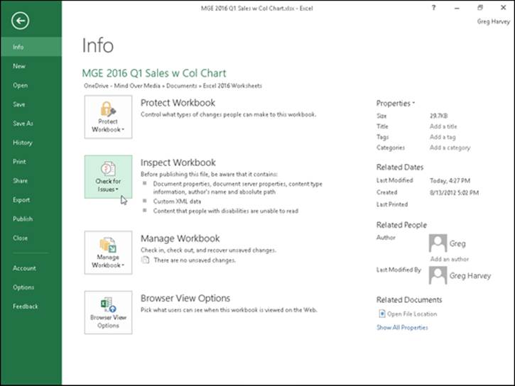
Figure 3-1: Checking a workbook’s properties in its Info screen in the Excel 2016 Backstage view.

Below the Check for Issues button, the Info screen contains a Manage Workbook button that, when clicked, gives you the following two options for recovering or clearing up draft versions of the workbook so that only the final version is available for sharing:

· Check Out to edit a private copy of the workbook and prevent others from making any changes to it

· Recover Unsaved Versions to enable you to browse all the versions of the current workbook that were closed without saving the final changes using Excel’s AutoRecover feature (see Book II, Chapter 1 for details)

At the very bottom of the Info screen, you find a Browser View Options button that, when clicked, opens the Browser View Options dialog box with a Show and Parameters tab. This tab enables you to control what parts of your workbook are displayed and can be edited when the file is shared online.

Adding properties to a workbook

You can add information about your workbook document (called metadata) in the Info panel in the Backstage view, using the various fields displayed in its right column (refer to Figure 3-1), which you open by selecting File  ⇒  Info or pressing Alt+FI. You can then use the metadata that you enter into the Title, Tags, Categories, and Author fields in the Info panel in all the Windows quick searches or file searches you perform. Doing so enables you to quickly locate the file for opening in Excel for further editing and printing or distributing to others to review.

When entering more than one piece of data into a particular field such as Title, Tags, or Categories, separate each piece with a comma. When you’re done adding metadata information to the fields, close the Info panel by clicking the File menu at the top of the panel or pressing Esc.

Click the Show All Properties link at the bottom of the right column of the Info screen containing the text boxes for particular document properties to add text boxes for additional document metadata fields including Comments, Template, Status, Subject, Hyperlink Base, Company, and Manager.

Digitally signing a document

Excel 2016 enables you to add digital signatures to the workbook files that you send out for review. After checking the spreadsheet and verifying its accuracy and readiness for distribution, you can (assuming that you have the authority within your company) digitally sign the workbook in one of two ways:

· Add a visible signature line as a graphic object in the workbook that contains your name, the date of the signing, your title, and, if you have a digital tablet connected to your computer or are running Excel on a touchscreen device, your inked handwritten signature.

· Add an invisible signature to the workbook indicated by the Digital Signature icon on the status bar and metadata added to the document that verifies the source of the workbook.

By adding a digital signature, you warrant the following three things about the Excel workbook you’re about to distribute:

· Authenticity: The person who signs the Excel workbook is the person he says he is (and not somebody else posing as the signer).

· Integrity: The content of the file has not been modified in any way since the workbook was digitally signed.

· Nonrepudiation: The signer stands behind the content of the workbook and vouches for its origin.

To make these assurances, the digital signature you add to the workbook must be valid in the following ways:

· The certificate that is associated with the digital signature must be issued to the signing publisher by a reputable certificate authority.

· The certificate must be current and valid.

· The signing publisher must be deemed trustworthy.

Microsoft partners such as ARX CoSign Digital Signatures, Avoco secure2trust, GlobalSign, or VeriSign offer digital ID services to which you can subscribe. As reputable certificate authorities, their protection services vouch for your trustworthiness as a signing publisher and the currency of the certificates associated with your digital signatures. In addition, they enable you to set the permissions for the workbook that determine who can open the document and how they can use it. To sign up with one of these services, choose the Add Signature Services option from the Add a Signature Line button’s drop-down menu and then follow the links on the Available Digital IDs Web page.

To add a digital signature to your finalized workbook, you follow these steps:

1. Inspect the worksheet data, save all final changes in the workbook file, and then position the cell pointer in a blank cell in the vicinity where you want the signature line graphic object to appear.

Excel adds the signature line graphic object in the area containing the cell pointer. If you don’t move the cell cursor to a blank area, you may have to move the signature line graphic so that graphic’s box doesn’t obscure existing worksheet data or other graphics or embedded charts.

2. Choose Insert  ⇒  Add a Signature Line  ⇒  Microsoft Office Signature Line in the Text group on the Ribbon (Alt+NG).

Excel displays the Signature Setup dialog box similar to the one shown in Figure 3-2.

3. Type the signer’s name into the Suggested Signer text box and then press Tab.

4. Type the signer’s title into the Suggested Signer’s Title text box and then press Tab.

5. Type the signer’s e-mail address into the Suggested Signer’s E-Mail Address text box.

6. (Optional) Select the Allow the Signer to Add Comments in the Sign Dialog check box if you want to add your own comments.

7. (Optional) Deselect the Show Sign Date in Signature Line check box if you don’t want the date displayed as part of the digital signature.

8. Click OK to close the Signature Setup dialog box.

Excel adds a signature line graphic object in the vicinity of the cell cursor with a big X that contains your name and title (shown in Figure 3-3).

9. Double-click this signature line graphic object or right-click the object and then choose Sign from its shortcut menu.

If you don’t have a digital ID with one of the subscription services or aren’t a Windows Live subscriber, Excel opens a Get a Digital ID alert dialog box asking you if you want to get one now. Click Yes and then follow the links on the Available Digital IDs Web page to subscribe to one.

Otherwise, Excel opens the Sign dialog box similar to the one shown in Figure 3-3.

10. Add your signature to the list box containing the insertion point.

To add your signature, click the Select Image link on the right, select a graphic file that contains a picture of your handwritten signature in the Select Signature Image dialog box, and then click Select. If you’re using a touchscreen device or your computer has a digital tablet connected to it, you add this signature by physically signing your signature with digital ink.

11. Click the Commitment Type drop-down list box and choose one of the options from its drop-down menu: Created and Approved This Document, Approved This Document, or Created This Document.

If you selected the Allow the Signer to Add Comments in the Sign Dialog check box in Step 6, the Sign dialog box contains a Purpose for Signing This Document text box that you fill out in Step 12.

12. Click the Purpose for Signing This Document text box and then type in the reason for digitally signing the workbook.

13. (Optional) Click the Details button to open the Additional Signing Information dialog box, where you can add the signer’s role and title as well as information on the place where the document was created.

14. (Optional) Click the Change command button to open the Windows Securities dialog box and then click the name of the person whose certificate you want to use in the list box and click OK.

By default, Excel issues a digital certificate for the person whose name is entered in the Suggested Signer text box back in Step 3. If you want to use a certificate issued to someone else in the organization, follow Step 12. Otherwise, proceed to Step 13.

15. Click the Sign button to close the Sign dialog box.

Excel closes the Sign dialog box.

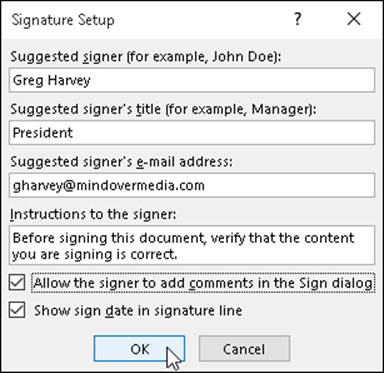
Figure 3-2: Filling out the signing information in the Signature Setup dialog box.

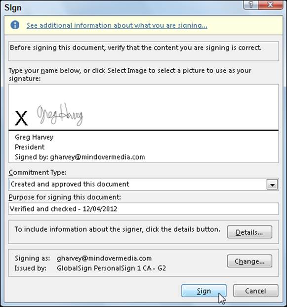
Figure 3-3: Filling in the signature in the Sign dialog box.

Immediately after closing the Sign dialog box, Excel adds your name to the digital signature graphic object and displays the MARKED AS FINAL alert at the top of the worksheet as shown in Figure 3-4.

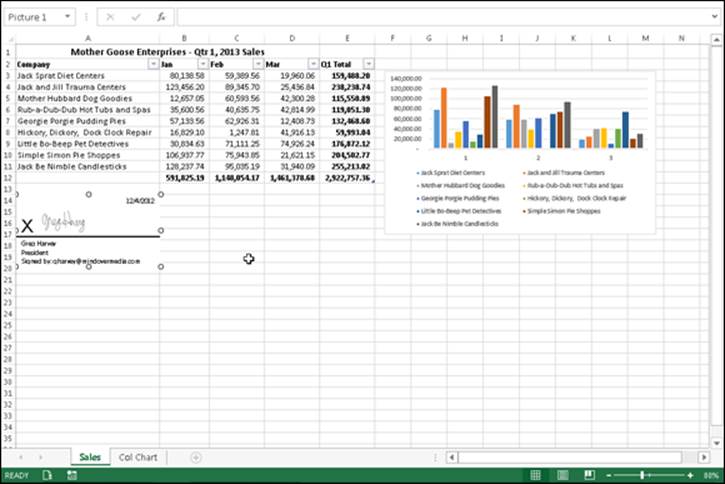
Figure 3-4: The workbook after adding the digital signature line graphic with the Signature task pane displayed.

To display all the information about the digital signature added to the workbook, right-click its graphic object and then choose Signature Details from its shortcut menu. To delete a digital signature from a workbook (which you need to do if you discover the sheets in the book require modification), right-click the signature graphic and then choose Remove Signature from its shortcut menu and click OK in its confirmation alert dialog box.

In place of a signature line, you can add a digital stamp (traditionally, in Asian countries such as China, Japan, and Korea, authorities sign a document not with a written signature but by affixing their official stamp to the document, usually in red ink). To literally add your stamp of approval, rather than your signature, to a workbook, choose the Stamp Signature Line option from the Signature Line button’s drop-down menu on the Insert tab of the Ribbon. You then follow steps very similar to those previously outlined for adding a digital signature line, except that you must select a graphic file that contains the image you want stamped in the workbook in lieu of your signature.

Workbook Sharing 101

If you save your workbooks online on your OneDrive or use Excel on a computer that’s connected to a local area network, you can share the spreadsheets that you create with others who have Internet or network access. Workbook sharing is perfect for spreadsheets that require frequent or regular data updates, especially for those whose data comes from several different departments, such as spreadsheets that track budgets or schedule projects that rely on input from many departments.

By sharing a workbook, you enable several people to edit its contents at the same time. Most often, you facilitate this process by saving the workbook file in a folder on your OneDrive and then sharing the workbook (see Book IV, Chapter 4 for details) or local area network drive (often mapped to a drive letter) to which everyone who needs to edit the spreadsheet has access.

You can share an Excel workbook on a local area network in one of two ways:

· Set up file sharing for the workbook by clicking the Share Workbook command button on the Ribbon’s Review tab (Alt+RW).

· Turn on change tracking for the workbook by choosing the Highlight Changes option from the Track Changes command button’s drop-down menu on the Ribbon’s Review tab (Alt+RGH).

Excel does not allow you to share a workbook with data lists that are formatted as tables (see Book II, Chapter 2). Before you can use the Share Workbook command button, you must first convert all your formatted tables into a normal range of cells. To do this, click a cell in each table and then click the Design tab on the Table Tools Contextual tab on the Ribbon. Finally, click the Convert to Range command button in the Tools group followed by the Yes button in the alert dialog box asking you to confirm this action. Excel then removes the filter buttons from the columns at the top of the data list while still retaining the original table formatting.

Whenever you share a workbook using either of these two methods, Excel automatically saves your workbook under the same filename with the shared information. The program then indicates that the workbook can now be shared by appending [Shared] to the workbook’s filename as it appears on the title bar of the Excel program window. When a second person on another computer on the network opens the shared workbook file, Excel opens a copy of the workbook file and the [Shared] indicator also appears on the title bar of his or her Excel program window appended to its filename.

This is in stark contrast to what happens when you try to open an unshared workbook on your computer that’s already open on another computer on the network. In that case, Excel displays a File in Use alert dialog box informing you that the workbook you want to open is already open. You can then choose between clicking the Read Only button to open the file in read-only mode (in which you can’t save your changes under the original filename) and clicking the Notify button to have the program open the file in read-only mode and then notify you when the other person closes the workbook so you can save your changes.

If you click the Notify button, as soon as the other person who was editing the workbook closes the file, Excel then displays a File Now Available alert dialog box, letting you know that the file is now available to save your editing. You then click its Read-Write button to close this alert dialog box, and after that, you’re free to save your editing changes to the original filename with the Save command (Ctrl+S).

Note that you don’t have to be running Excel 2016 on your computer in order to open and edit a shared workbook. Workbook sharing is supported by the earlier versions of Excel (2007 and 97 through 2003). You can’t, however, save changes to a shared workbook if you’re using a version earlier than Excel 2007.

Also note that when you make changes to a shared workbook, Excel uses your username to identify the modifications that you made. To modify your username, you edit the contents of the User Name text box on the General tab of the Excel Options dialog box (File  ⇒  Options or Alt+FT).

When you share a workbook, Excel disables some of the program’s editing features so they can’t be used in editing the shared spreadsheet. The following tasks are not enabled in a shared workbook:

· Deleting worksheets from the workbook

· Merging cells in the worksheets of a workbook

· Applying conditional formats to the cells of the worksheets (although all conditional formats in effect before you share the workbook remain in effect)

· Setting up or applying data validation to cells of the worksheets (although all data validation restrictions and messages remain in effect in the shared workbook)

· Inserting or deleting blocks of cells in a worksheet (although you can insert or delete entire columns and rows from the sheet)

· Drawing shapes and adding text boxes (see Book V, Chapter 2 for details)

· Assigning passwords for protecting individual worksheets or the entire workbook (although all protection and passwords defined prior to sharing the workbook remain in effect — see Book IV, Chapter 1 for details on protecting worksheets)

· Grouping or outlining data in a worksheet (see Book II, Chapter 4 for details)

· Inserting automatic subtotals in a worksheet (see Book VI, Chapter 1 for details)

· Creating data tables or pivot tables in a worksheet (see Book VII, Chapters 1 and 2 for details)

· Creating, revising, or assigning macros (although you can run macros that were created in the worksheet before it was shared, provided that they don’t perform any operations that aren’t supported by a shared workbook — see Book VIII, Chapter 1 for details)

Turning on file sharing

The first way to share a workbook is by turning on file sharing as follows:

1. Open the workbook to be shared, convert any data lists formatted as tables to cell ranges, and then make any last-minute edits to the file, especially those that are not supported in a shared workbook.

Keep in mind when making these last-minute changes that when you share a workbook, some of Excel’s editing features become unavailable to you and any others working in the file. (Refer to the list in the previous section for exactly which features are unavailable.)

Before turning on file sharing, you may want to save the workbook in a special folder on a network drive to which everyone who is to edit the file has access.

2. Choose File  ⇒  Save As or press Alt+FA and then select your OneDrive or the network drive on the Save As screen followed by the folder in the Save As dialog box in which you want to the make the change tracking version of this file available before you click the Save button.

3. Click the Share Workbook command button on the Review tab of the Ribbon or press Alt+RW.

Excel opens a Share Workbook dialog box (similar to the one shown in Figure 3-5). This dialog box contains two tabs: an Editing tab that enables you to turn on file sharing for all the users who have the file open, and an Advanced tab, where you control how the amount of time that changes is tracked and how updates are handled.

4. Select the Allow Changes by More Than One User at the Same Time check box on the Editing tab.

By default, Excel maintains a Change History log for 30 days. If you wish, you can use the Advanced tab settings to modify whether Excel maintains this Change History log (necessary if you want to reconcile and merge changes) or to change how long the program saves this log. You can also change when changes are updated, how conflicts are handled, and whether your print settings and data filtering settings are shared.

5. (Optional) Click the Advanced tab and then change the options on this tab that affect how long a change log is maintained and how editing conflicts are handled.

See the following section, “Modifying the Workbook Share options,” for details on changing these settings.

6. Click the OK button to close the Share Workbook dialog box.

As soon as Excel closes the Share Workbook dialog box, an alert dialog box appears, telling you that Excel will now save the workbook and asking you if you want to continue.

7. Click the OK button in the Microsoft Excel alert dialog box to save the workbook with the file sharing settings.

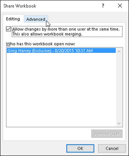
Figure 3-5: Turning on file sharing on the Editing tab of the Share Workbook dialog box.

Immediately after you click OK and close the alert dialog box, Excel saves the workbook, and the [Shared] indicator appears at the end of the filename on the Excel program window’s title bar.

Modifying the Share Workbook options

As soon as you turn on file sharing for a workbook, Excel also turns on a Change History log that records all the changes made by different individuals to the same workbook file. You can use the Change History log to view information about the various changes made to a shared workbook and to determine which of the changes to retain if conflicting changes are made by different people to the same cells of a workbook. You can also use the Change History log when merging changes from different copies of the same workbook into a single file.

By default, Excel maintains the Change History log for a period of 30 days from the date that you first share the workbook. If you wish, you can change the length of time that Excel maintains the Change History log or even, in rare circumstances, elect to not keep the log.

To make changes to the length of time that Excel maintains the Change History log, you click the Advanced tab in the Share Workbook dialog box (Alt+RW), as shown in Figure 3-6. This tab contains the following sections with options for not only changing how long the Change History log is maintained, but also controlling when and how updates are handled:

· Track Changes: Enables you to modify how long Excel keeps the Change History log by entering a new value in the Keep Change History For text box or selecting a new value with the spinner buttons. Click the Don’t Keep Change History option button should you ever decide that you don’t need the Change History log.

· Update Changes: Enables you to select when changes made by different users are saved. By default, Excel saves changes when the file is saved. To have the program save changes every so many minutes, click the Automatically Every option button and then enter the number of minutes for the save interval in the Minutes text box or select this interval value with its spinner buttons. When automatically saving changes every so many minutes, by default Excel saves only your changes while showing you changes made to the workbook by others. To have the program just display the changes made to the file by others when the save interval is reached without saving your changes, click the Just See Other Users’ Changes option button.

· Conflicting Changes Between Users: Enables you to select how changes made to the same cells of a shared workbook by different users are treated. By default, Excel is set to ask you which user’s changes to accept and which to deny. If you want Excel to accept the changes made by any user at the time she saves the workbook, click the Changes Being Saved Win option button.

· Include in Personal View: Enables you to determine which of your personal settings are saved when you save the workbook. By default, Excel saves both your personal print settings (including such things as page breaks, changes to the print area, and changes to the printing settings — see Book II, Chapter 5 for details) and the filtering settings you select with the AutoFilter buttons. (See Book VI, Chapter 2 for details.) Deselect the Print Settings and/or Filter Settings check boxes at the bottom of the Advanced tab if you decide that you don’t need these settings saved as part of the shared workbook.

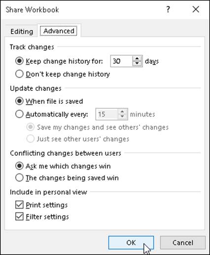
Figure 3-6: Modifying the sharing options on the Advanced tab of the Share Workbook dialog box.

Turning on change tracking

The second way to share a workbook is by turning on change tracking. When you do this, Excel tracks all changes you make to the contents of the cells in the shared workbook by highlighting their cells and adding comments that summarize the type of change you make. When you turn on change tracking, Excel automatically turns on file sharing along with the workbook’s Change History log.

To turn on change tracking in a workbook, you take these steps:

1. Open the workbook for which you want to track changes and that you wish to share, convert any data lists formatted as tables to cell ranges, and then make any last-minute edits to the file, especially those that are not supported in a shared workbook.

When making these last-minute changes, keep in mind that, when you share a workbook, some of Excel’s editing features become unavailable to you and any others working in the file. (Refer to the “Workbook Sharing 101” section, earlier in this chapter, for a list of exactly which features are unavailable.)

Before turning on file sharing, you may want to save the workbook in a special folder on a network drive to which everyone who is to edit the file has access.

2. Choose File  ⇒  Save As or press Alt+FA and then select your OneDrive or the network drive on the Save As screen; then, in the Save As dialog box, select the folder in which you want to the make the change tracking version of this file available before you click the Save button.

3. Choose the Highlight Changes option from the Track Changes command button’s drop-down menu on the Review tab or press Alt+RGH.

Doing this opens the Highlight Changes dialog box, shown in Figure 3-7, where you turn on change tracking and indicate which changes to highlight.

4. Select the Track Changes While Editing check box.

Doing this turns on change tracking and automatically turns on file sharing for the workbook.

By default, Excel selects the When combo box and chooses the All option from its drop-down menu to have all changes made to the workbook tracked. To track the changes only from the time you last saved the workbook, choose the Since I Last Saved item from the When drop-down menu. To track all changes that you’ve not yet reviewed (and decided whether to accept), you choose the Not Yet Reviewed item from the When drop-down menu. (Most often, you want this option so that you can use the Accept/Reject Changes option on the Track Changes command button’s drop-down menu to review each person’s changes and decide whether to keep them.) To track changes from a particular date, choose Since Date from the When drop-down menu: Excel then inserts the current date into the When combo box, which you can then edit, if necessary.

5. (Optional) If you don’t want to track all changes in the workbook, click the When drop-down button and then choose the menu item from its drop-down menu (Since I Last Saved, Not Yet Reviewed, or Since Date).

By default, Excel tracks the changes made by anybody who opens and edits the workbook (including you). If you want to exempt yourself from change tracking or restrict it to a particular user, select the Who check box and then choose Everyone But Me or the user’s name from the Who drop-down menu.

6. (Optional) If you want to restrict change tracking, click the name of the person to whom you want to restrict change tracking in the Who drop-down menu.

Note that selecting any option from the Who drop-down menu automatically selects the Who check box by putting a check mark in it.

By default, changes made to any and all cells in every sheet in the workbook are tracked. To restrict the change tracking to a particular range or nonadjacent cell selection, select the Where check box and then select the cells.

7. (Optional) If you want to restrict change tracking to a particular cell range or cell selection in the workbook, click the Where combo box and then select the cell range or nonadjacent cell selection in the workbook.

Clicking the Where text box and selecting a cell range in the workbook automatically selects the Where check box by putting a check mark in it.

By default, Excel highlights all editing changes in the cells of the worksheet on the screen by selecting the Highlight Changes on Screen check box. If you don’t want the changes marked in the cells, you need to deselect this check box.

8. (Optional) If you don’t want changes displayed in the cells onscreen, click the Highlight Changes on Screen check box to clear its check mark.

Note that after you finish saving the workbook as a shared file, you can return to the Highlight Changes dialog box and then select its List Changes on a New Sheet check box to have all your changes listed on a new worksheet added to the workbook. Note too, that if you select this check box when the Highlight Changes on Screen check box is selected, Excel both marks the changes in their cells and lists them on a new sheet. If you deselect the Highlight Changes on Screen check box while the List Changes on a New Sheet check box is selected, Excel just lists the changes on a new worksheet without marking them in the cells of the worksheet.

9. Click the OK button to close the Highlight Changes dialog box.

As soon as Excel closes the Highlight Changes dialog box, an alert dialog box appears, telling you that Excel will now save the workbook and asking you if you want to continue.

10. Click the OK button in the Microsoft Excel alert dialog box to save the workbook with the change tracking and file sharing settings.

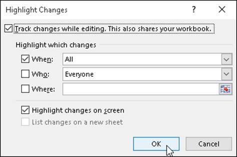
Figure 3-7: Turning on change tracking in the Highlight Changes dialog box.

After you turn on change tracking in a shared workbook, Excel highlights the following changes:

· Changes to the cell contents, including moving and copying the contents to new cells in the worksheet

· Deletion of the cell contents

· Insertion of new rows, columns, or cells in a worksheet

When change tracking is turned on in a workbook, the program does not, however, highlight any of these changes:

· Formatting changes made to the cells

· Hidden or unhidden rows and columns in the worksheet

· Renamed sheet tabs in the workbook

· Insertion or deletion of a worksheet in the workbook

· Comments added to the cells

· Changes to cell values resulting from the recalculation of formulas or to cells whose values depend upon those formulas

In highlighting changes you make to the shared workbook, Excel draws a thin line (in another color — usually blue) around the borders of the cell, while at the same time placing a triangle of the same color in the cell’s upper-left corner. When you position the thick white-cross mouse or Touch pointer on a highlighted cell, Excel displays a comment indicating the change made to the cell along with the date and time it was made and who made it, as shown in Figure 3-8.

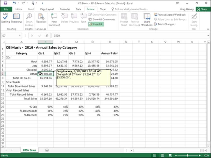
Figure 3-8: Displaying the comment added to a cell highlighted by change tracking.

When you turn on change tracking, you also necessarily turn on file sharing, and when file sharing is in effect, you can’t make certain kinds of editing changes. For a complete list of these changes, refer back to the section, “Workbook Sharing 101,” earlier in this chapter.

Merging changes from different users

At some point after sharing a workbook, you’ll want to update the workbook to incorporate the changes made by different users. When merging changes, you may also have to deal with conflicting changes made to the same cells and decide which changes to accept and which to reject. After you’ve merged all the input and decided how to deal with all the conflicting changes, you may even want to turn off file sharing to prevent users from doing any further editing.

To be able to compare versions of a shared workbook and incorporate changes from your co-workers, you need to add the Compare and Merge Workbooks command button to the Quick Access toolbar:

1. Click the Customize Quick Access Toolbar button at the end of the Quick Access toolbar and then choose the More Commands option.

Excel opens the Excel Options dialog box with the Quick Access Toolbar tab selected.

2. Choose the Commands Not in the Ribbon option from the Choose Commands From drop-down menu.

Excel displays a list of all the commands not currently on the Ribbon in the list box beneath the Choose Commands From drop-down box.

3. Click the Compare and Merge Workbooks item in the list box below and then click the Add button.

The Compare and Merge Workbooks item appears below the last item in the Quick Access Toolbar list box on the right side of the Excel options dialog box.

4. Click the OK button to close the Excel Options dialog box.

The Compare and Merge Workbooks button appears at the end of the Quick Access toolbar. (Its icon is an outlined circle.)

When you click the Compare and Merge Workbooks button that you added to the Quick Access toolbar with the original workbook file open in Excel, the program opens the Select Files to Merge Into Current Workbook dialog box. Here, you select the drive and folder that contain the copies of the shared workbook file edited by your co-workers.

Resolving conflicts

Should Excel identify cells in the workbook that contain conflicting changes (that is, different values placed in the same cell by different users) after you select their files in the Select Files to Merge Into Current Workbook dialog box, it flags the cells in the original workbook open in Excel and then displays the conflict in the Resolve Conflicts dialog box. To accept your change to the cell in question, you click the Accept Mine button. To accept the change made by another user, you click the Accept Other button instead.

After you accept your change or the other user’s change in the case of the first conflict, Excel flags the next case and displays a description of the conflicting values in the Resolve Conflicts dialog box. When you finish accepting or rejecting your change or the one made by another user for the last conflicting value, Excel automatically closes the Resolve Conflicts dialog box, and you can save your changes to the workbook by choosing File  ⇒  Save or by pressing Ctrl+S.

If you want Excel to accept only your changes in all cases of conflicting values, click the Accept All Mine button. To have Excel reject all your changes and accept all those made by others, click the Accept All Others button instead.

If you know that you always want all your changes to be accepted in the case of conflicting values, open the Share Workbook dialog box (Alt+RW) and then click the Changes Being Saved Win option button on the Advanced tab before you click OK. If you prefer to have your changes (including conflicting ones) automatically saved at set intervals, click the Automatically option button and set the number of minutes between saves in the Minutes text box before you click OK.

Accepting or rejecting highlighted changes

When you turn on change tracking for a workbook, you can decide which changes to accept or reject by choosing the Accept/Reject Changes option from the Track Changes command button’s drop-down menu on the Ribbon’s Review tab (or pressing Alt+RGC). When you do this, Excel reviews all the highlighted changes made by you and others who’ve worked on the shared file, enabling you to accept or reject individual changes.

When you first choose the Accept/Reject Changes option, Excel displays the alert dialog box, informing you that Excel will save the workbook. When you click OK to close this alert dialog box, the program opens the Select Changes to Accept or Reject dialog box, which contains the same three check boxes and associated drop-down items (When, Who, and Where) as the Highlight Changes dialog box shown earlier in Figure 3-7.

By default, the When check box is selected along with the Not Yet Reviewed setting in the Select Changes to Accept or Reject dialog box. When this setting is selected, Excel displays all the changes in the workbook that you haven’t yet reviewed for everyone who has modified the shared file. To review only those changes you made on the current date, choose the Since Date item from the When drop-down menu. To review changes made since a particular date, edit the current date in the Since Date drop-down list.

To review only changes that other people have made, only those changes you’ve made, or only those changes a particular co-worker has made, choose the appropriate item (Everyone But Me, your name, or another user’s name) from the Who drop-down menu. If you want to restrict the review to a particular range or region of a worksheet, click the Where combo box and then select the range or nonadjacent cell ranges with the cells to review.

After you select which changes to review in the Select Changes to Accept or Reject dialog box, click the OK button. Excel then closes this dialog box, highlights the cell in the worksheet that contains the first change to review, and opens the Accept or Reject Changes dialog box (similar to the one shown in Figure 3-9), where you indicate whether to accept or reject the change. To accept the change, you click the Accept button. To reject the change and keep the original value, you click the Reject button instead. Excel then highlights the next cell in the worksheet that needs reviewing, while at the same time displaying a description of the change in the Accept or Reject Changes dialog box.

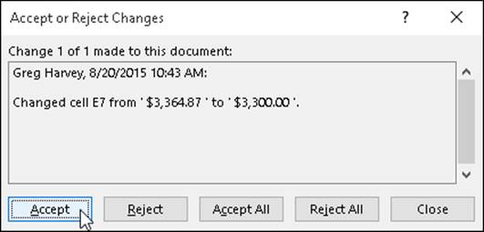
Figure 3-9: Deciding whether or not to accept a change in the Accept or Reject Changes dialog box.

If you know ahead of time that you want to accept or reject all the changes that have been made since you last reviewed the workbook or the date you specified, click the Accept All button or the Reject All button, respectively. When you accept or reject the last change identified in the workbook, the Accept or Reject Changes dialog box automatically closes, and you can then save the workbook (Ctrl+S) with the editing changes made as a result of this review.

How to stop sharing a workbook

If you decide that you no longer want to share a particular workbook, you can turn off file sharing. To do this, open the Share Workbook dialog box (Alt+RW) and remove the check mark from the Allow Changes by More Than One User at the Same Time check box on the Editing tab before you click OK.

As soon as you click OK, Excel displays an Information alert dialog box indicating that your action is about to remove the workbook from shared use and, at the same time, erase the Change History log. It also informs you that users who are currently editing this workbook will be unable to save their changes even if you should later change your mind and turn the file sharing back on again.

Because users are prevented from saving their changes and the Change History log is erased as soon as you turn off file sharing and make the workbook once again exclusive, you don’t ever want to turn off file sharing until after you’re sure that you have everybody’s comments and changes saved to the workbook and have reviewed and merged the changes you want to keep.

If you’re sure that you’ve met these two conditions, you can click the Yes button in the Information alert dialog box to turn off file sharing and once again make the workbook your exclusive property. Click the No button, however, to abort this procedure if you have any doubt about having all your users’ changes erased.

It’s always a good idea to inform the users of your shared workbook of your intention to remove the file from shared use well in advance of the actual date. Your best bet is to e-mail each user and let him or her know exactly the date and time after which the workbook will no longer be shared and open to their edits. That way, each person on the team knows the exact time after which his or her changes and comments will no longer be accepted (which is often a good inducement for the procrastinators on the team to send you their last-minute suggestions and changes).

Removing a user from the shared workbook

Sometimes, rather than preventing everyone from sharing a particular workbook, you may only need to stop particular users from being able to edit it. To remove a specific user from sharing in the editing, you open the Share Workbook dialog box (Alt+RW), click the name of the person you want to remove in the Who Has the Workbook Open Now list box, and then click the Remove User button.

As soon as you click this button, Excel displays an alert dialog box informing you that if the user you selected is currently editing the workbook, your action will prevent him or her from saving the workbook so that all unsaved work is automatically lost. To proceed with removing the user, click the OK button in this alert dialog box. To abandon the removal until after you’ve verified that the user isn’t currently editing the file, click the Cancel button instead.

Workbooks on Review

Even if you don’t save your workbooks on a OneDrive or use Excel on a network, you still can add your comments to the cells of a workbook that ask for clarification or suggest changes, and then you can distribute copies of the workbook by e-mail to other people who need to review and, perhaps, respond to your remarks. Excel makes it easy to annotate the cells of a worksheet, and the command buttons on the Review tab of the Ribbon make it easy to review these notes prior to e-mailing the workbook to others who have to review the comments, and even reply to suggested changes.

If you’re running Excel 2016 on a computer equipped with a digital tablet or on a touchscreen device such as a Windows tablet, the Review tab of your Ribbon has a Start Inking command button (not included on this tab when running Excel on a regular PC). When you click the Start Inking command button, Excel adds an Ink Tools contextual tab to the Ribbon. You can then use the command buttons on its Pens tab to highlight and mark up various parts of the spreadsheet with digital ink.

Adding comments

You can add comments to the current cell by clicking the New Comment command button on the Ribbon’s Review tab or by pressing Alt+RC. Excel responds by adding a Comment box (similar to the one shown in Figure 3-10) with your name listed at the top (or the name of the person who shows up in the User Name text box on the Personalize tab of the Excel Options dialog box). You can then type the text of your comment in this box. When you finish typing the text of the note, click the cell to which you’re attaching the note or any other cell in the worksheet to close the Comment box.

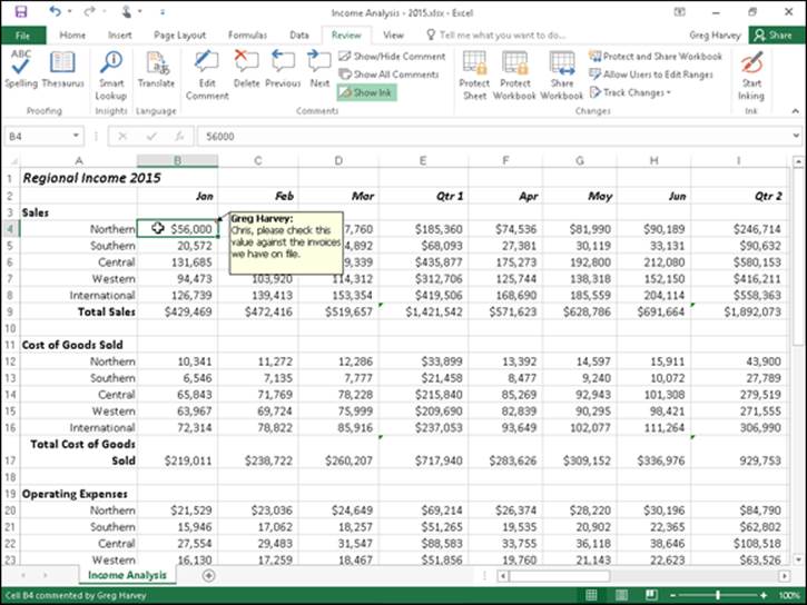
Figure 3-10: Adding comments to various cells of a worksheet.

Displaying and hiding comments

Excel indicates that you’ve attached a comment to a worksheet cell by adding a red triangle to the cell’s upper-right corner. To display the Comment box with its text, you position the thick, white-cross mouse pointer on this red triangle, or you can click the Show All Comments command button on the Review tab (Alt+RA) to display all comments in the worksheet.

When you display a comment by positioning the mouse pointer on the cell’s red triangle, the comment disappears as soon as you move the pointer outside the cell. When you display all the comments on the worksheet by clicking the Show All Comments command button on the Review tab, you must click the Show All Comments button a second time before Excel closes their Comment boxes (or press Alt+RA).

Editing and formatting comments

When you first add a comment to a cell, its Comment box appears to the right of the cell with an arrow pointing to the red triangle in the cell’s upper-right corner. If you need to, you can reposition a cell’s Comment box and/or resize it so that it doesn’t obscure certain cells in the immediate region. You can also edit the text of a comment and change the formatting of the text font.

To reposition or resize a Comment box or edit the note text or its font, you make the cell current by putting the cell cursor in it, and then click the Edit Comment command button, which replaces the New Comment button as the first button in the Comments group on the Review tab of the Ribbon, or press Alt+RT. (You can also do this by right-clicking the cell and then choosing Edit Comment from the cell’s shortcut menu.)

Whichever method you use, Excel then displays the cell’s Comment box and positions the insertion point at the end of the comment text. To reposition the Comment box, position the mouse pointer on the edge of the box (indicated with cross-hatching and open circles around the perimeter). When the mouse or Touch pointer assumes the shape of a white arrowhead pointing to a black double-cross, you can then drag the outline of the Comment box to a new position in the worksheet. After you release the mouse button, Excel draws a new line ending in an arrowhead from the repositioned Comment box to the red triangle in the cell’s upper-right corner.

When editing and formatting the comments you’ve added to the worksheet, you can do any of the following:

· To resize the Comment box, you position the mouse pointer on one of the open circles at the corners or in the middle of each edge on the box’s perimeter. When the mouse pointer changes into a double-headed arrow, you drag the handle of the Comment box until its dotted outline is the size and shape you want. (Excel automatically reflows the comment text to suit the new size and shape of the box.)

· To edit the text of the comment (when the insertion point is positioned somewhere in it), drag the I-beam mouse pointer through text that needs to be replaced or press the Backspace key (to remove characters to the left of the insertion point) or Delete key (to remove characters to the right). You can insert new characters in the comment to the right of the insertion point by simply typing them.

· To change the formatting of the comment text, select the text by dragging the I-beam mouse pointer through it, and then click the appropriate command button in the Font and Alignment groups on the Home tab of the Ribbon. (You can use Live Preview to see how a new font or font size, on its respective drop-down menu, looks in the comment, provided that these drop-down menus don’t cover the Comment box in the worksheet.)

You can also right-click the text and choose Format Comment from the shortcut menu. Doing this opens the Format Comment dialog box (with the same options as the Font tab of the Format Cells dialog box) where you can change the font, font style, font size, font color, or add special effects including underlining, strikethrough, as well as super- and subscripting.

When you finish making your changes to the Comment box and text, close the Comment box by clicking its cell or any of the other cells in the worksheet.

Deleting comments

When you no longer need a comment, you can delete it by selecting its cell before you do any of the following:

· Choose the Comments option from the Clear button’s drop-down menu on the Home tab of the Ribbon or press Alt+HEM.

· Click the Delete command button in the Comments group on the Review tab of the Ribbon or press Alt+RD.

· Right-click the cell and then choose Delete Comment from its shortcut menu.

If you delete a comment in error, you can restore it to its cell by clicking the Undo command button on the Quick Access toolbar or pressing Ctrl+Z.

Marking up a worksheet with digital ink

If you’re running Excel 2016 with a computer connected to a digital tablet or on a touchscreen, you can mark up your worksheets with digital ink. Excel 2016 running on a computer equipped with a digital tablet or running on a touchscreen device contains a Start Inking command button located at the very end of the Ribbon’s Review tab. When you tap this command button (or press Alt+RK), Excel displays a Pens tab on the Ink Tools contextual tab.

By default, Excel chooses the felt tip pen as the pen type for annotating the worksheet with digital ink. If you’d prefer to use a ballpoint pen or highlighter in marking up the worksheet, click the Pen command button or Highlighter command button in the Pens group.

When using the highlighter or either of the two pen types (felt tip or ballpoint pen), you can select a nib from the Pens palette displayed in the middle of the Pens tab. You can also select a new line weight for the ink by choosing the point size (running from 3/4 all the way up to 6 points) from the Thickness command button’s drop-down menu. You can also select a new ink color (yellow being the default color for the highlighter, red for the felt tip pen, and black for ballpoint pen) by clicking its color swatch on the Color command button’s drop-down palette.

After you select the pen nib, color, and line weight, you can use your finger or the stylus that comes with your digital tablet to mark up the spreadsheet as follows:

· To highlight data in the spreadsheet with the highlighter, drag the highlight mouse pointer through the cells (just as though you had an actual yellow highlighter in your hand).

· To circle data in the spreadsheet with the felt tip pen, drag the pen tip mouse pointer around the cells in the worksheet.

· To add a comment with the ballpoint pen, drag the pen tip mouse pointer to write out your text in the worksheet.

Figure 3-11 shows a copy of the Income Analysis worksheet after I used the Highlighter and Pen commands on the Pens tab to highlight cell B4 in the worksheet, circle it, and write the comment “verify” in digital ink.

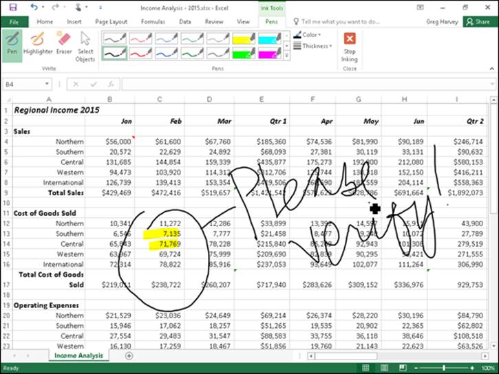
Figure 3-11: Adding inked comments to a worksheet with my finger on a Windows tablet.

If you make a mistake with ink, you need to remove it and start over again. To delete the ink, select the Eraser command button in the Write group and then tap somewhere on the highlighting, drawing, or handwriting you want to erase with the eraser mouse pointer. (Sometimes you have to drag through the ink to completely remove it.) Then, reselect the highlighter or felt tip or ballpoint pen and reapply your ink annotation.

When you finish marking up the worksheet with ink, click the Stop Inking command button on the Pens tab of the Ink Tools contextual tab. Excel then closes the Ink Tools contextual tab, once again displaying only the normal Ribbon tabs.

Use the Show Ink command button on the Review tab (Alt+RI) to hide and redisplay the inked comments that you add to your worksheet. The first time you tap this command button when the inked comments you’ve added are displayed onscreen, Excel hides them. Tap the Show Ink command button again, when you want all your inked comments redisplayed in the worksheet.

After marking a workbook up with your comments, you can then share it with clients or co-workers either by sending an e-mail message inviting them to review the workbook or actually sending them a copy as an e-mail attachment. (See Book IV, Chapter 4 for details.)