Microsoft Office for iPad Step by Step (2015)
Part 3: Microsoft Excel for iPad
CHAPTER 7 Store and retrieve data
CHAPTER 8 Process and present numeric data
7. Store and retrieve data
In this chapter
![]() Create workbooks
Create workbooks
![]() Create and manage worksheets
Create and manage worksheets
![]() Enter and edit data on worksheets
Enter and edit data on worksheets
![]() Modify columns and rows
Modify columns and rows
![]() Modify cells and cell content
Modify cells and cell content
![]() Manage the display of data
Manage the display of data
Excel provides a practical yet powerful data management framework. You can store massive quantities of data within this deceptively simple structure, analyze that data, and present the resulting information in a variety of structures. The key ingredient in all of these tasks is the original data. The final presentation or analysis is only as good as the data it’s based on. This “garbage in, garbage out” rule is true for many business tools, programs, and processes; Excel is no exception.
A worksheet can contain a vast amount of static and calculated data. You can structure worksheet content so that data is presented correctly on the screen and when printed, and you can format data so that it is easier for readers to locate and understand specific categories of information.
Practice files
For this chapter, use the practice files from the iPadOfficeSBS\Ch07 folder. For practice file download instructions, see the Introduction.
This chapter guides you through procedures related to creating workbooks and worksheets, managing worksheets and worksheet elements, populating worksheets with text or numeric data, modifying worksheet structure, and formatting data for presentation. It also includes procedures for efficiently displaying, filtering, and sorting data to provide specific information and perspectives.
The Excel feature set
Excel for iPad has only a subset of the features of the full program. Here is a brief comparison of the features in each version. You can save and edit workbooks in a shared storage location by using multiple versions.
Excel for iPad features
After you sign in by using a Microsoft account, you can do the following:
![]() Create, manage, and print workbooks and worksheets.
Create, manage, and print workbooks and worksheets.
![]() Format, find, replace, sort, and filter content.
Format, find, replace, sort, and filter content.
![]() Insert pictures that are available on your iPad.
Insert pictures that are available on your iPad.
![]() Create formulas, Excel tables, and charts.
Create formulas, Excel tables, and charts.
![]() Display conditional formatting and interact with data validation options, PivotTables, and comments.
Display conditional formatting and interact with data validation options, PivotTables, and comments.
The following premium features require that you sign in by using an account that is associated with a qualified Office 365 subscription:
![]() Insert and edit WordArt.
Insert and edit WordArt.
![]() Customize PivotTable styles and layouts.
Customize PivotTable styles and layouts.
![]() Add custom colors to shapes, and add shadows and reflection styles to pictures.
Add custom colors to shapes, and add shadows and reflection styles to pictures.
Excel Online features
You can use Excel Online to do the following:
![]() Coauthor workbooks in real time and edit macro-enabled workbooks.
Coauthor workbooks in real time and edit macro-enabled workbooks.
![]() Display three-dimensional charts, slicers, Power Pivot tables and charts, and Power View sheets.
Display three-dimensional charts, slicers, Power Pivot tables and charts, and Power View sheets.
![]() Embed workbooks on webpages.
Embed workbooks on webpages.
![]() Send and compile surveys.
Send and compile surveys.
For more information about Excel Online, visit technet.microsoft.com/en-us/library/excel-online-service-description.aspx.
Excel desktop version features
The desktop versions of Excel have the most functionality. For example, you can use Excel 2013 on a computer running Windows to do the following:
![]() Display multiple views of worksheets, split windows, multiple windows, and very large workbooks.
Display multiple views of worksheets, split windows, multiple windows, and very large workbooks.
![]() Display and edit workbooks from remote storage locations offline.
Display and edit workbooks from remote storage locations offline.
![]() Insert equations and symbols.
Insert equations and symbols.
![]() Insert pictures from local and online sources.
Insert pictures from local and online sources.
![]() Create SmartArt diagrams, and capture screen images.
Create SmartArt diagrams, and capture screen images.
![]() Copy and paint formatting.
Copy and paint formatting.
![]() Insert header and footer content.
Insert header and footer content.
![]() Configure page layout options.
Configure page layout options.
![]() Use apps and web resources to enhance content.
Use apps and web resources to enhance content.
![]() Apply conditional formatting and sparklines.
Apply conditional formatting and sparklines.
![]() Sort and filter data by using slicers and timelines.
Sort and filter data by using slicers and timelines.
![]() Create and edit three-dimensional charts.
Create and edit three-dimensional charts.
![]() Define named ranges.
Define named ranges.
![]() Audit formulas and require manual calculation of formulas.
Audit formulas and require manual calculation of formulas.
![]() Analyze data by using the Quick Analysis tool.
Analyze data by using the Quick Analysis tool.
![]() Create data validation rules, consolidate data, and perform conditional analysis.
Create data validation rules, consolidate data, and perform conditional analysis.
![]() Group, subtotal, and outline data.
Group, subtotal, and outline data.
![]() Create PivotTables, Power Pivot data models, and Power View sheets.
Create PivotTables, Power Pivot data models, and Power View sheets.
![]() Create, save, and run macros.
Create, save, and run macros.
![]() Use Office proofing tools.
Use Office proofing tools.
![]() Protect workbook elements.
Protect workbook elements.
![]() Track changes, insert comments, and respond to comments.
Track changes, insert comments, and respond to comments.
Create workbooks
As with other Office files, you can create a blank Excel workbook or a workbook that contains content from a template. Excel templates focus more on purpose than on appearance; they provide structure and functionality for specific types of information.
The templates that are available from within Excel for iPad range from a simple to-do list to a complex financial report and include expense reports, sales reports, household budgets, marketing budgets, time sheets, invoices, loan calculators, and ledgers. Most of the templates include basic calculations; some include advanced calculations and visual representations of data. Even if these don’t meet your specific needs, they can serve as a good example of ways to collect, track, process, or present data.
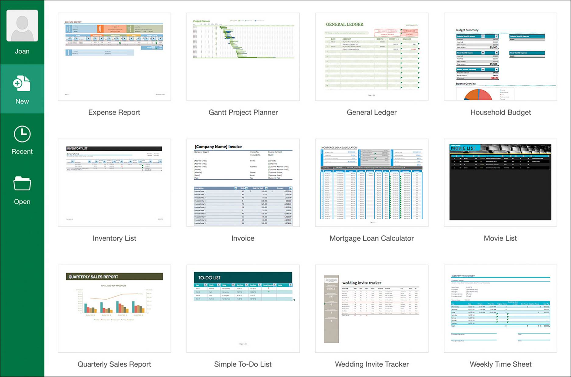
Excel for iPad has 16 built-in templates, including the blank workbook
Only the templates that are installed with Excel for iPad are available from the New page. Other workbook templates are available for Excel Online, and hundreds are available from within the desktop versions of Excel. If you create a workbook based on one of these templates and save the workbook to a shared storage location, you can then open and edit the workbook on your iPad.
You can access templates for Excel Online from your iPad by using Safari or another web browser to visit store.office.live.com/templates/templates-for-Excel.
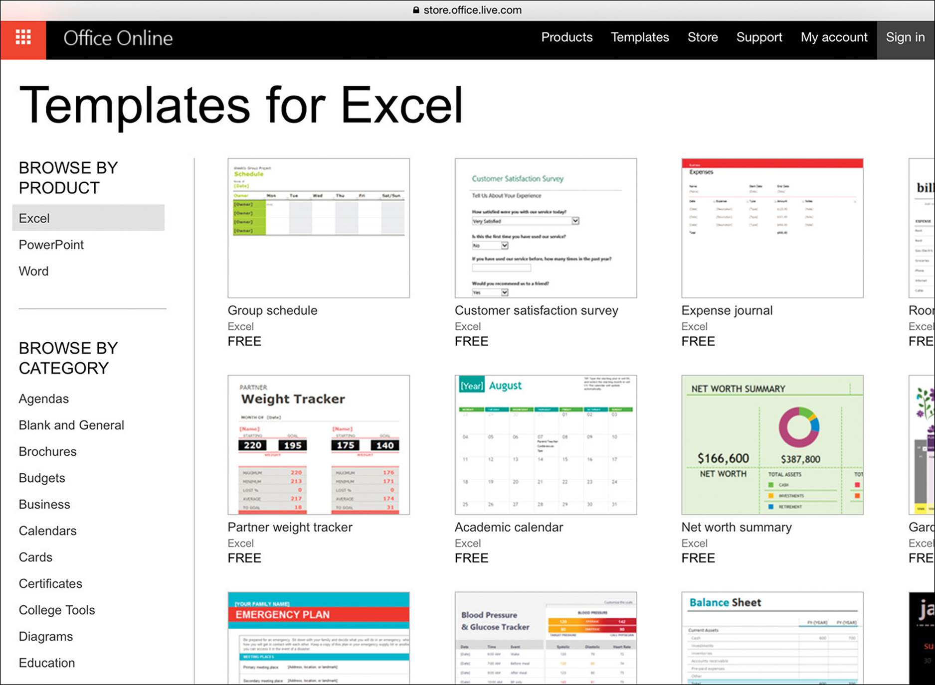
Additional templates are available online
To create a blank Excel workbook
1. In the Backstage view, on the File bar, tap New.
2. On the New page, tap New Blank Workbook.
To create a workbook from a built-in template
1. In the Backstage view, on the File bar, tap New.
2. Locate and then tap the thumbnail of the workbook template you want to use.
 Tip
Tip
The processes of creating workbooks from Excel and Excel Online templates for use in Excel for iPad are the same as those of creating documents from Word and Word Online templates for use in Word for iPad. For step-by-step instructions, see “Create documents from templates” in Chapter 4, “Create professional documents.” For general information about creating files in Excel for iPad and other Office apps, see “Create, open, and save files” in Chapter 3, “Create and manage files.”
Create and manage worksheets
Workbooks provide structure for the storage of information, but you store the information on worksheets within the workbook. A worksheet provides a seemingly simple cellular structure that can store more than 17 billion data points.
Tip
The current worksheet size limitation is 16,384 columns by 1,048,576 rows (which won’t be a limitation for most Excel users). A single cell can contain up to 32,767 characters.
You don’t have to store all your data on one worksheet. You can organize information on separate worksheets so that the content of each worksheet is easier to review and manage. You don’t even have to store all related data on the same worksheet—you can easily reference data on other worksheets for purposes such as performing calculations or creating reports. You can also reference data in other workbooks, so it isn’t necessary to have a copy of a worksheet that you reference from multiple workbooks in each of those workbooks.
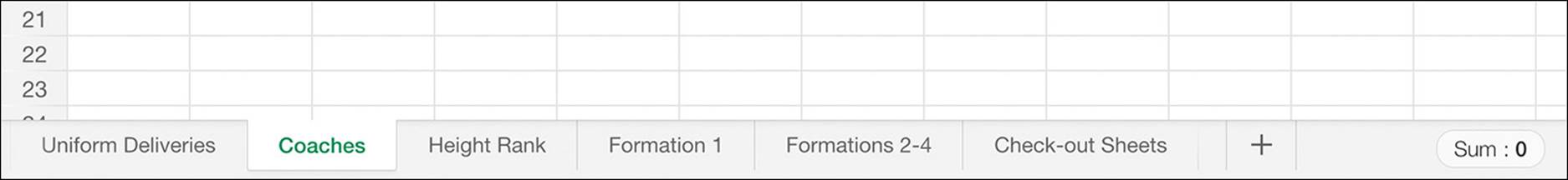
Scroll sideways to access worksheet tabs that don’t fit in the sheet tab area
 See Also
For information about referencing other worksheets and workbooks, see “Perform data-processing operations” in Chapter 8, “Process and present numeric data.”
Add, rename, and remove worksheets
A new, blank Excel workbook contains one worksheet named Sheet1. You can add more worksheets to the workbook for the purpose of storing or displaying data, and give each worksheet a meaningful name. If you want to use an existing worksheet as a starting point for another, you can make a copy of the worksheet, rename the copy, and then modify the data on the copy. The data on the copy is not linked to the data on the original worksheet.
To select or display a worksheet
1. In the sheet tab area, tap the worksheet tab.
To add a worksheet to a workbook
1. In the sheet tab area, to the right of the existing worksheet tabs, tap the Insert Worksheet button, which is labeled with a plus sign (+).
To create a copy of a worksheet
1. Display the worksheet that you want to copy.
2. Tap the active worksheet tab to display the shortcut bar.
3. On the shortcut bar, tap Duplicate.
To rename a worksheet
1. Display the worksheet that you want to rename.
2. Double-tap the active worksheet tab to activate the worksheet name for editing and display the on-screen keyboard.
3. Enter the new worksheet name, and then do one of the following:
• Tap anywhere on the worksheet.
• On the on-screen keyboard, tap Done or tap the Keyboard key.
 Important
The Undo command does not reverse actions such as renaming, hiding, and deleting that you perform on worksheet tabs.
To delete a worksheet from a workbook
1. Display the worksheet that you want to delete.
2. Tap the active worksheet tab. Then on the shortcut bar, tap Delete.
Tip
You can display charts and other visual representations of data on worksheets with their supporting data, or you can move them onto their own worksheets. In some versions of Excel, you can export a chart from a worksheet to its own chart sheet. For more information, see “Display data in charts” in Chapter 8, “Process and present numeric data.”
Move and hide worksheets
Many workbooks contain multiple worksheets. The data you store or display on individual worksheets might exist independently or interact with content on other worksheets. For example, you might:
![]() Store data for individual time periods or projects on separate worksheets.
Store data for individual time periods or projects on separate worksheets.
![]() Store static information such as resources, list options, and holiday dates on one worksheet and reference that information in calculations on several other worksheets.
Store static information such as resources, list options, and holiday dates on one worksheet and reference that information in calculations on several other worksheets.
![]() Display a chart on a worksheet that is separate from the data that supports it.
Display a chart on a worksheet that is separate from the data that supports it.
![]() Display data from multiple worksheets on a summary worksheet.
Display data from multiple worksheets on a summary worksheet.
You can organize worksheets in a workbook by reordering them.
If you don’t need to have the information on a worksheet immediately available, or if you want to protect or conceal a worksheet, you can hide it. Hiding a worksheet removes the worksheet tab from the sheet tab area on the status bar but doesn’t remove any data.
To move a worksheet within a workbook
1. Display the worksheet that you want to move.
2. In the sheet tab area, tap and hold the active worksheet tab, and then drag it to its new location.
To hide a worksheet
1. Display the worksheet that you want to hide.
2. In the sheet tab area, tap the active worksheet tab. Then on the shortcut bar, tap Hide.
To unhide a worksheet
1. Tap the active worksheet tab.
2. On the shortcut bar, tap Unhide to display a list of the hidden worksheets in the workbook.
3. In the list, tap the name of the worksheet that you want to unhide.
Show and hide worksheet elements
Data stored in an Excel worksheet is organized in columns and rows. The junction of each column and row is a cell, and this is where you enter data.
An empty worksheet resembles a piece of graph paper, with each cell outlined so you can easily locate it. Lettered headings across the top of the worksheet identify specific columns, and numbered headings down the left side of the worksheet identify specific rows. Worksheet tabs at the bottom of the window identify worksheets within the workbook.
You can hide all these user interface elements to display more of a worksheet or to focus on the worksheet content. You can also hide the Formula Bar when it isn’t required, so that it appears only temporarily while you edit cell content.

A summary sheet displays information based on the data on other worksheets
Hiding the Formula Bar or worksheet tabs affects all the worksheets in a workbook. Hiding the gridlines or headings affects only the active worksheet. Excel preserves the gridline and heading settings, so if you exit and reopen a workbook the gridlines and headings on each worksheet will be as you left them.
To hide Excel user interface elements
1. On the View tab, tap the Formula Bar, Gridlines, Headings, or Sheet Tabs slider to change its background to white.
To temporarily display the Formula Bar
1. Double-tap a worksheet cell to activate it for editing.
To permanently redisplay Excel user interface elements
1. On the View tab, tap the Formula Bar, Gridlines, Headings, or Sheet Tabs slider to change its background to green.
Tip
Exiting and reopening a workbook redisplays the Formula Bar and worksheet tabs if they’ve been hidden.
Enter and edit data on worksheets
Excel for iPad has a Ready mode and an Edit mode. When you’re working with the structural aspects of cells, Excel is in Ready mode and the active cell or cell range has selection handles. When you’re working with cell content, Excel is in Edit mode and there are no selection handles.
When you enter Edit mode, the Formula Bar opens above the worksheet, and the on-screen keyboard opens below the worksheet. This compresses the workspace significantly. You can orient your iPad horizontally to display more columns or vertically to display more rows.
Tip
If your iPad is connected to an external keyboard, the on-screen keyboard doesn’t open in Edit mode. You can perform many operations by using keyboard shortcuts on an external keyboard. For a complete list of keyboard shortcuts, see the Appendix, “Touchscreen and keyboard shortcuts.”
When Excel is in Edit mode, you can select individual cells, columns, or rows, but you can’t expand the selection directly on the iPad. (You can do so from a connected external keyboard.) Selecting a column or row activates the first cell in the column or row for editing.
Select cells, columns, and rows
A key step in the process of entering, modifying, or formatting worksheet content is selecting the cell or cells you want to work with. You can use these selection methods in the Excel for iPad touch interface:
![]() To select a cell, tap it once.
To select a cell, tap it once.
TIP Selecting a cell or range of cells displays selection handles in the upper-left and lower-right corners of the selection and a related statistic on the status bar. For more information, see the sidebar “Quickly display statistics” in Chapter 8, “Process and present numeric data.”
![]() To select a range of cells, select the upper-left cell in the range, and then drag the lower-right handle to the lower-right cell of the range or flick the handle down or to the right to select all populated cells in that direction (from the current cell to the next blank cell).
To select a range of cells, select the upper-left cell in the range, and then drag the lower-right handle to the lower-right cell of the range or flick the handle down or to the right to select all populated cells in that direction (from the current cell to the next blank cell).
![]() To select a column, tap the column heading (the colored block above the worksheet that is labeled with a letter). Selecting a column displays selection handles on the left and right sides of the column and the content of the first visible cell of the column in the Formula Bar.
To select a column, tap the column heading (the colored block above the worksheet that is labeled with a letter). Selecting a column displays selection handles on the left and right sides of the column and the content of the first visible cell of the column in the Formula Bar.
![]() To select a row, tap the row heading (the colored block to the left of the worksheet that is labeled with a number). Selecting a row displays selection handles on the top and bottom of the row and the content of the first visible cell of the row in the Formula Bar.
To select a row, tap the row heading (the colored block to the left of the worksheet that is labeled with a number). Selecting a row displays selection handles on the top and bottom of the row and the content of the first visible cell of the row in the Formula Bar.
TIP Selecting a column or row displays a shortcut bar of relevant commands. To close the shortcut bar and maintain the selection, tap an empty area of the ribbon.
![]() To select multiple columns or rows, select one column or row and then drag the handles to select adjacent columns or rows.
To select multiple columns or rows, select one column or row and then drag the handles to select adjacent columns or rows.
TIP When an Excel table is active, tapping the column or row heading might select only the corresponding column or row of the table.
![]() To select an entire worksheet, tap the Select All button, which is located at the junction of the column headings and row headings and is labeled with a triangle that points toward the worksheet.
To select an entire worksheet, tap the Select All button, which is located at the junction of the column headings and row headings and is labeled with a triangle that points toward the worksheet.
When you enter Edit mode from a cell that already contains content, or switch to a cell that contains content while you’re in Edit mode, Excel displays and selects the cell content in the Formula Bar.
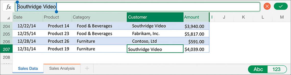
The content of the active cell shifts to the far left when Excel is in Edit mode
Tip
It’s easy to forget that you’re in Edit mode. If you can’t select cells, columns, or rows in the worksheet, check the Formula Bar for the telltale Cancel and Finish buttons.
In Excel for iPad, you enter and edit all text in the Formula Bar. The cell immediately displays the text, but the cursor is never active in the cell as it is in the desktop versions of Excel. In addition to the standard letters and numbers, you can enter the special characters that are available from the standard, number, and function online keyboards. Most notably, you can insert a line break within text to manually wrap cell content in a specific location.
If the data you want to enter follows a specific pattern such as 5, 10, 15, 20 or Monday, Tuesday, Wednesday, Thursday, you can establish the pattern and then have Excel continue the pattern and fill in the rest of the cells for you.
If the data you want to store in a worksheet already exists in another location, you can copy it from the source and paste it into the worksheet. This avoids the errors that can occur when entering data manually. The process of pasting content in Excel is the same as in other Office for iPad apps. If you paste a table into a worksheet, the table cells will map to the worksheet cells so that the table retains its structure.
Tip
You can locate information within a workbook by searching for values, formula elements, or named objects. For information about searching Excel workbooks, see “Search file content” in Chapter 3, “Create and manage files.”
Display and hide the shortcut bar
Regardless of your experience with Excel, it can take some practice to master the techniques for selecting and manipulating content by touch on an iPad rather than by using a mouse. When you are working with content in Excel for iPad, the shortcut bar can be very convenient because it provides access to the most frequently used commands for a selected entity. It can also be inconvenient because sometimes it opens on top of content or tools that you want to work with.
Tapping a cell and then tapping it again displays the shortcut bar for the cell. (This action of tapping twice isn’t the same as double-tapping; it’s slower and has a different result.) Tapping a column or row heading once selects the column or row and also displays the shortcut bar.
You can perform most common tasks from the context-specific shortcut bar
You can hide the shortcut bar and still maintain the selection by tapping a colored part of the ribbon.
Important
You perform many tasks in Word for iPad, Excel for iPad, and PowerPoint for iPad by using the same processes. Common processes include those for giving commands in the Office user interface and for opening, saving, searching, and distributing files. For more information, see Chapter 3, “Create and manage files.”
To switch from Ready mode to Edit mode
1. Do any of the following:
• Double-tap a cell.
• Select a cell and then tap the Formula Bar.
• Begin typing on a connected external keyboard.
• Press Ctrl+2 on a connected external keyboard.
To switch from Edit mode to Ready mode
1. Do any of the following:
• To complete the edit and move to the next cell, tap the Return key on the on-screen keyboard or press the Enter key on a connected external keyboard.
• To complete the edit and stay in the current cell, tap the Finish button (labeled with a check mark) at the right end of the Formula Bar or the Keyboard key on the on-screen keyboard.
• To complete the edit and expand the selection, hold down the Shift key and press an arrow key.
• To discard the edit, tap the Cancel button (labeled with an X) at the right end of the Formula Bar.
To enter or edit cell content
1. Switch to Edit mode, and then enter text from the on-screen keyboard.
Or
From Ready mode or Edit mode, enter text from a connected external keyboard.
To insert a line break in cell content
1. In Edit mode, position the cursor where you want the line break.
2. In the upper-right corner of the on-screen keyboard, tap the Function button (labeled 123) to display the function keyboard.
See Also
For more information about the function keyboard, see “Perform data-processing operations” in Chapter 8, “Process and present numeric data.”
3. On the function keyboard, press and hold the Return key (labeled with a curved arrow) to display the Line Break key, and then slide your finger to the Line Break key.
Tip
The Line Break key and other hidden keys are visible only until you lift your finger from the screen. For more information about hidden keys, see “Perform data-processing operations” in Chapter 8, “Process and present numeric data.”
To move the content of one or more cells
1. Select the cell or cells.
2. Tap and hold the selection until an animated dotted line outlines the selection. Then without lifting your finger, drag the selected content to the new location.
To fill cells with data that matches a pattern
1. In Edit mode, enter the first two items of the data series into adjacent cells.
2. Switch to Ready mode.
3. Tap the first cell and then drag the selection handle to select the second cell.
4. Tap the selection to display the shortcut bar.
5. On the shortcut bar, tap Fill. Note the arrows that appear on the right and bottom sides of the selected cell.
6. Drag the right-pointing arrow to the right to fill the series over, or drag the downward-pointing arrow down to fill the series down.
Tip
You can automatically fill series containing days of the week, months of the year, numbers, text, dates, times, and more.
To delete cell content
1. Select the range of cells you want to clear.
2. On the shortcut bar, tap Clear.
Or
On the on-screen keyboard or a connected external keyboard, tap or press the Delete key.
Modify columns and rows
A new worksheet has columns of equal width and rows of equal height. A standard letter-size printed page displays approximately 9 columns and 47 rows at the default sizes. The number of columns and rows visible on screen varies based on the dimensions and resolution of your screen. The content that you enter in a worksheet will rarely fit perfectly in the default structure, especially if you’re entering text content.
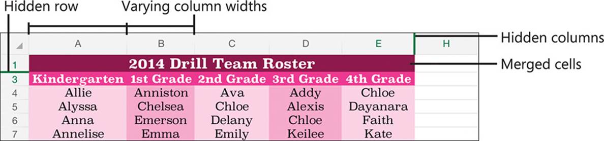
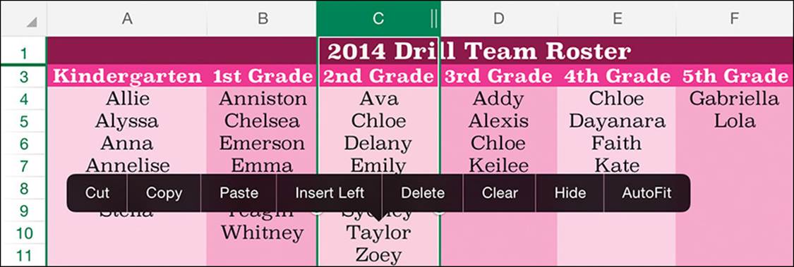
You can vary the size and visibility of columns and rows to suit your data
Resize columns and rows
After you enter data in a worksheet, you can easily modify the structure of the worksheet to fit the content. You can change the size of columns and rows so their content is visible on screen and when printed. You can change the width of a column or height of a row manually or by using the AutoFit feature to size the column or row to fit its contents.
Tip
You can’t display or set the specific column width or row height measurements in Excel for iPad; you can adjust them only by dragging or by using the AutoFit feature.
To fit a column or row to its contents
1. Double-tap the column or row heading.
Or
Select the column or row, and then tap AutoFit on the shortcut bar.
To change the width of a column
1. Select the column. Notice the handle that appears on the right side of the column heading.
2. Drag the handle to the left to make the column narrower or to the right to make the column wider.
To change the height of a row
1. Select the row. Notice the handle that appears below the row heading.
2. Drag the handle upward to make the row shorter or downward to make the row taller.
Insert and delete columns and rows
After you populate a data range or table, you can easily insert additional columns or rows into the range or table without overwriting existing data; existing columns shift to the right and rows shift down. Excel automatically updates any references in the workbook to the cells that shift to accommodate the insertion.
See Also
For information about referencing cells and cell ranges, see “Perform data-processing operations” in Chapter 8, “Process and present numeric data.”
You can specify the insertion location for columns or rows, or the columns or rows you want to delete, by selecting them, or by selecting only representative cells.
If a column or row containing the data you want to insert already exists, you can move that column or row to a different location or copy it to another location. When you delete columns or rows, Excel shifts the remaining content to fill the gap and updates any cell references in the workbook to reflect the change.
Tip
Note the difference between deleting and clearing cells. When you delete a cell, it is completely removed from the worksheet, and other cells move to replace it. When you clear a cell, the content of the cell is deleted, but the cell structure remains in place.
To insert a blank column
1. Select the column, or any cell in the column, that is in the position where you want to insert the blank column.
Tip
If you want to insert multiple columns in one location, drag the selection handle to the right to select the number of columns you want to insert.
2. On the shortcut bar, tap Insert Left.
Or
On the Home tab, tap the Insert & Delete Cells button, and then tap Insert Sheet Columns.
To move or copy a column to another location
1. Select the column you want to move or copy.
Tip
If you want to move or copy multiple contiguous columns, drag the selection handles to select the adjacent columns.
2. On the shortcut bar, do one of the following:
• If you want to move the selected column, tap Cut.
• If you want to duplicate the selected column, tap Copy.
3. Select the column that is in the position where you want to place the column.
4. On the shortcut bar, tap Insert Left.
Or
On the Home tab, tap the Insert & Delete Cells button, and then tap Insert Sheet Columns.
To insert a blank row
1. Select the row, or any cell in the row, that is in the position where you want to insert the blank row.
Tip
If you want to insert multiple rows in the same location, drag the selection handle down to select the same number of rows that you want to insert.
2. On the shortcut bar, tap Insert Above.
Or
On the Home tab, tap the Insert & Delete Cells button, and then tap Insert Sheet Rows.
To move or copy a row to another location
1. Select the row you want to move or copy.
Tip
If you want to move or copy multiple contiguous rows, drag the selection handles to select the adjacent rows.
2. On the shortcut bar, do one of the following:
• If you want to move the selected row, tap Cut.
• If you want to duplicate the selected row, tap Copy.
3. Select the row that is in the position where you want to place the cut or copied rows.
4. On the shortcut bar, tap Insert Above.
Or
On the Home tab, tap the Insert & Delete Cells button, and then tap Insert Sheet Rows.
To delete a column
1. Select the column, or any cell in the column, that you want to delete.
Tip
If you want to delete multiple contiguous columns, drag the selection handles to select the adjacent columns or cells.
2. On the Home tab, tap the Insert & Delete Cells button, and then tap Delete Sheet Columns.
To delete a row
1. Select the row, or any cell in the row, that you want to delete.
Tip
If you want to delete multiple contiguous rows, drag the selection handles to select the adjacent rows or cells.
2. On the Home tab, tap the Insert & Delete Cells button, and then tap Delete Sheet Rows.
Hide and unhide columns and rows
If a data range includes a column or row of information that you either don’t want to display or don’t want to include in a chart, but that you don’t want to delete, you can hide it instead. The headings of a hidden column or row don’t change, so you can identify locations of hidden columns and rows by the missing headings and the thick lines that replace them.
Important
You can’t hide columns or rows of Excel tables when you are working with a workbook in Excel for iPad. If you need to hide a table column or row, you can convert the table to a data range, hide the column or row, and then convert the data range to a table. For more information about Excel tables, see “Create and manage Excel tables” in Chapter 8, “Process and present numeric data.”
To hide a column or row
1. Tap the heading of the column or row you want to hide.
Tip
If you want to hide multiple contiguous columns or rows, drag the selection handles to select the adjacent columns or rows.
2. On the shortcut bar, tap Hide.
To unhide a hidden column or row
1. Tap the column heading to the left of the hidden column, then drag the right selection handle to the right to select the next visible column.
Or
Tap the row heading above the hidden row, then drag the lower selection handle down to select the next visible row.
2. On the shortcut bar, tap Unhide.
Modify cells and cell content
Sometimes you need to modify the structure of a worksheet on the cell level rather than modifying an entire column or row. For example, you might need to remove only one entry from a column that contains a list of entries. Deleting (clearing) the cell content would leave a gap—you must delete the entire cell to close the gap.
Insert and delete cells
When you insert or delete individual cells from a worksheet, you must stipulate the direction in which Excel should shift the worksheet content that is below and to the right of the cell.
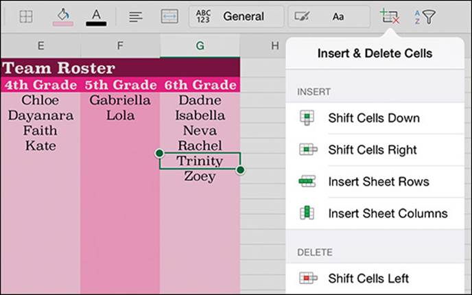
You choose the direction to shift content when inserting or deleting cells
To insert a blank cell in a populated range
1. Select the cell that is located where you want the blank cell.
2. On the Home tab, tap the Insert & Delete Cells button, and then tap Shift Cells Down or Shift Cells Right, depending on where you want to move the adjacent cells.
To insert multiple cells
1. Select the range of cells that occupy the space in which you want to insert the new blank cells.
2. On the Home tab, tap the Insert & Delete Cells button, and then tap Shift Cells Down or Shift Cells Right, depending on where you want the surrounding cells to be moved.
To delete a cell
1. Select the cell (or range of cells) that you want to delete.
2. On the Home tab, tap the Insert & Delete Cells button, and then tap Shift Cells Left or Shift Cells Up, depending on where you want the surrounding cells to be moved.
Modify cell structure
By default, text content that exceeds the width of its column extends across adjacent columns if they are empty. If the adjacent column contains content, only the text that fits in the first column is visible. If you don’t want to resize the column to fit the text, you can wrap the text to display it on multiple lines.
Tip
In Excel for iPad, you can wrap the content of a single cell or multiple cells, but not of an entire column.
If a number is too wide to be displayed in a column, Excel displays the result in scientific notation, or displays number signs (#) instead of the number. You can’t wrap a long number, but you can widen the column or change the font size to fit the number in the cell.
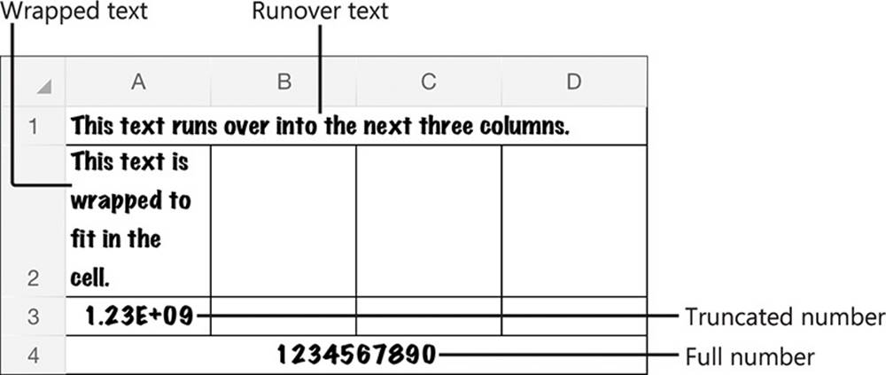
Methods of handling content that exceeds the width of the cell
Sometimes it is appropriate to merge the content of multiple cells into one cell; for example, to indicate that a heading or label applies to multiple columns or rows. A merged cell occupies the space of the original cells.
Important
When you merge multiple cells, Excel keeps only the data from the upper-left cell, and discards the other values. If the other cells contain data that you want to keep, move the data before merging the cells.
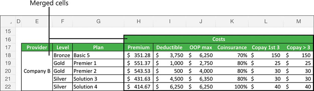
You can merge cells vertically, horizontally, or both
Tip
Merged cells can interfere with some types of operations on the surrounding columns or rows, such as filling cell data. If this happens, you can unmerge the cells, perform the operation, and then remerge the cells.
To wrap or unwrap text
1. Select the cell you want to format, and then tap the selected cell.
Or
Select multiple contiguous cells that you want to format.
2. On the shortcut bar, tap Wrap or Unwrap.
To merge a range of cells
1. Select the cells you want to combine.
2. On the Home tab, tap the Merge & Center button.
Format cell appearance
You can format worksheet content to help people identify key information. Beyond the standard font formatting options, you can add shading (also called fill color) and borders to cells. You can fill cells and apply borders independently or as part of a preset cell style. Some of the cell styles available in Excel are intended to convey specific information and others are linked to the workbook theme.
Tip
Conditional formatting is an incredibly useful tool for exposing trends in numeric data. You can’t apply or modify conditional formatting rules in Excel for iPad, but you can open worksheets that include conditional formatting rules created in other versions of Excel, and the rules function correctly in Excel for iPad.
All the cell styles are purely decorative. None of the styles that are designated as titles and headings actually affect the structure of the content or link to an outline level, as headings in a Word document do.
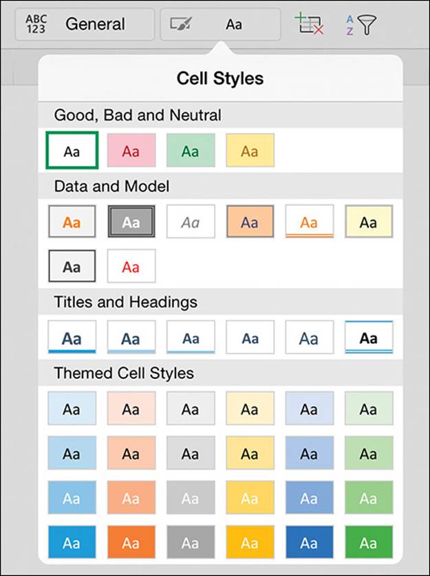
You can use cell styles to add visual interest and meaning to a cell
See Also
For information about changing the font, size, color, and style of text, see “Change the appearance of text” in Chapter 4, “Create professional documents.”
A workbook can store many types of numeric data, and not all of these numbers should be displayed or processed in the same way. You can format specific types of numbers to display correctly and so that Excel correctly recognizes whether to process the number as a value or as something else (such as a date).
Excel for iPad includes 11 categories of number formats:
![]() General This is the default format for numbers. It permits Excel to process numbers in mathematic operations and to display numbers by using scientific notation if necessary to fit within the cell.
General This is the default format for numbers. It permits Excel to process numbers in mathematic operations and to display numbers by using scientific notation if necessary to fit within the cell.
![]() Text This number format instructs Excel to display and process the number exactly as you enter it. It is particularly useful for numbers with leading zeros and long numbers, such as credit card numbers, that Excel would otherwise change to scientific notation.
Text This number format instructs Excel to display and process the number exactly as you enter it. It is particularly useful for numbers with leading zeros and long numbers, such as credit card numbers, that Excel would otherwise change to scientific notation.
![]() Accounting This format allows you to display a specific number of decimal places and a currency symbol, which is left-aligned in the cell so the values are easier to read.
Accounting This format allows you to display a specific number of decimal places and a currency symbol, which is left-aligned in the cell so the values are easier to read.
![]() Currency This format allows you to display a specific number of decimal places and a currency symbol, which is flush against the numbers. You can also specify the format of negative values.
Currency This format allows you to display a specific number of decimal places and a currency symbol, which is flush against the numbers. You can also specify the format of negative values.
![]() Date This format allows you to choose from among many standard options for displaying short and long dates to regional standards.
Date This format allows you to choose from among many standard options for displaying short and long dates to regional standards.
![]() Fractions This format expresses a decimal number as the equivalent fraction. You can specify the denominator or degree of precision up to 1/999.
Fractions This format expresses a decimal number as the equivalent fraction. You can specify the denominator or degree of precision up to 1/999.
![]() Number This format allows you to display a specific number of decimal places and specify whether to display the thousands separator and how to format negative numbers.
Number This format allows you to display a specific number of decimal places and specify whether to display the thousands separator and how to format negative numbers.
![]() Percentage This format displays a decimal number as the equivalent percentage followed by the percent symbol. If you want to display more precise percentages, you can specify the number of decimal places.
Percentage This format displays a decimal number as the equivalent percentage followed by the percent symbol. If you want to display more precise percentages, you can specify the number of decimal places.
![]() Scientific This format expresses a number in scientific notation. You can specify the number of decimal places of the expression.
Scientific This format expresses a number in scientific notation. You can specify the number of decimal places of the expression.
![]() Time This format allows you to choose from among many standard options for displaying times or date/time combinations to regional standards.
Time This format allows you to choose from among many standard options for displaying times or date/time combinations to regional standards.
![]() Special This category includes region-specific formats for numbers such as ZIP codes, postal codes, phone numbers, and Social Security numbers.
Special This category includes region-specific formats for numbers such as ZIP codes, postal codes, phone numbers, and Social Security numbers.
To add, change, or remove cell borders
1. Select the cell or cell range for which you want to format borders.
2. On the Home tab, tap the Cell Borders button.
3. On the Cell Borders menu, do one of the following:
• To apply a border to only one side of the selection, tap Bottom Border, Top Border, Left Border, or Right Border.
• To apply borders to multiple sides of the selection, tap All Borders, Outside Borders, or Thick Box Border.
• To remove all cell borders, tap No Border.
Tip
Additional border styles and customization options are available in the desktop versions of Excel. If a worksheet cell has a border style that is unavailable in Excel for iPad, you can apply the border to other cells by copying the cell and then pasting only the format to the other cells.
To specify or remove a cell background color
1. Select the cell or cell range you want to format.
2. On the Home tab, tap the Fill Color button.
3. On the Fill Color menu, do one of the following:
• Tap the color you want to apply.
• Tap No Fill to remove any applied color.
Tip
The Fill Color dialog box displays six variations of each theme color, 10 standard colors, and a Custom Color link that displays a spectrum you can select a color from.
To apply a preset cell style
1. Select the cell or cell range you want to format.
2. On the Home tab, tap the Cell Styles button.
3. On the Cell Styles menu, tap the style you want to apply.
To specify a number format
1. Select the cell or cell range you want to format.
2. On the Home tab, tap the Number Formatting button.
3. On the Number Formatting menu, do one of the following:
• To apply the default format for a category, tap the category name.
• To apply a specific number format, tap the i (the information symbol) to the right of the category name. Set the format-specific options, and then tap away from the menu to close it.
Tip
You can summarize large amounts of data for analysis by using a PivotTable, and present visual representations of data as charts. For more information about these presentation tools, see Chapter 8, “Process and present numeric data.”
Manage the display of data
When a worksheet contains a large amount of data, it can be challenging to review the data, especially on a small screen such as that of the iPad. If you need to keep all the data at hand, you can rotate the iPad to display more columns or more rows at the same magnification; hide headings, worksheet tabs, and other user interface elements to increase the space available for the worksheet; or zoom out to display more content in the app window. You can freeze the column and row labels so they stay visible—and identify the on-screen content—while you flick through the data range.
If you’re focusing on specific data, you can hide columns and rows that you don’t need to review. To really narrow things down, you can hide data that isn’t relevant to your needs by filtering it, and then present different aspects of the data for evaluations by changing the sort order.
See Also
For information about hiding user interface elements, columns, and rows, see “Create and manage worksheets” and “Modify columns and rows” earlier in this chapter.
Freeze panes
When a worksheet contains more data than you can display on one screen, you must scroll vertically or horizontally to display additional fields and entries. When you scroll a worksheet that contains a data range, the lettered column headings and numbered row headings can help you to identify the visible data, but it’s easy to lose track of specific fields or entries. To simplify this process, you can “freeze” the columns and rows that contain labels so they stay in place when you flick through a worksheet.
For a typical data range that starts in the upper-left corner of a worksheet (cell A1), the top row contains the column labels and the first column contains the row labels. Because this is common, Excel provides options to freeze the top row and the first column. Alternatively, you can select the first cell that you want to scroll and then choose the option to freeze the worksheet panes above and to the left of that.
Frozen panes are indicated by thin lines on the worksheet that start between the column headings or row headings. When the display of gridlines is turned off, the lines are visible in the worksheet background.
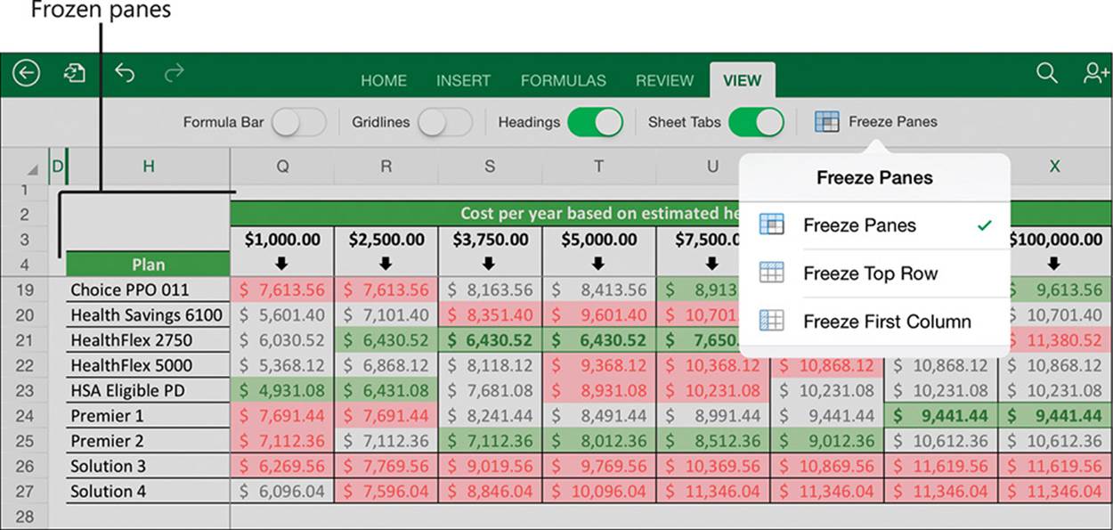
You can freeze panes at any location in a worksheet
To freeze the panes to the left of and above a specific cell
1. Position the worksheet so that the rows you want to have visible after you freeze the panes are the first rows in the window.
Important
In Excel for iPad, freezing rows prevents the frozen rows from scrolling, so if you want to have multiple rows visible when scrolling, ensure that they are exposed before you freeze the rows.
2. Select the first cell that you want to scroll (this cell will not be frozen).
3. On the View tab, tap Freeze Panes. Then on the Freeze Panes menu, tap Freeze Panes.
To freeze the first visible column
1. Position the worksheet so that the one column you want to freeze as you scroll horizontally is the first column in the window.
2. On the View tab, tap Freeze Panes. Then on the Freeze Panes menu, tap Freeze First Column.
To freeze the first visible row
1. Position the worksheet so that the one row you want to freeze as you scroll vertically is the first row in the window.
2. On the View tab, tap Freeze Panes. Then on the Freeze Panes menu, tap Freeze Top Row.
To unfreeze panes
1. On the View tab, tap Freeze Panes.
2. On the Freeze Panes menu, tap the current selection, and then tap a blank area of the ribbon to close the menu.
Sort and filter data
A key feature of Excel is the ability to locate specific data or data that meets specific requirements. You can use the search function to locate specific text or characteristics and then move among the results one by one. For many purposes, however, it’s more useful to manipulate the data range to display data in a certain arrangement or to display only (and all) the records that share specific characteristics.
You can sort a data range or Excel table by the entries in any column to present the data in different ways. For example, if you have a list of products offered by different companies at different prices, you can sort the data by company name, by product name, or by price. Then you can narrow down the options by filtering the data to display only (and all) the records that share specific characteristics.
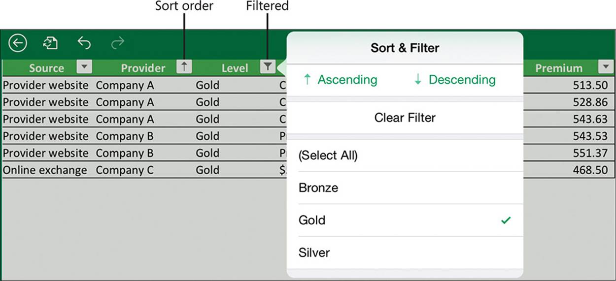
Filtering displays only the rows that contain the selected entry
 Tip
Tip
You can filter a data range by more than one column to display only entries that meet multiple criteria. In Excel for iPad, you can sort a data range by only one column at a time; you can’t perform multilevel sorts from the Sort & Filter menu.
Filtering is off by default for data ranges, but you can easily turn it on. When you do, Excel evaluates the data and displays a Sort & Filter button at the right edge of each data column heading. The button label changes to indicate the column status, as follows:
![]() When a column is neither sorted nor filtered, the button is labeled with a downward-pointing triangle.
When a column is neither sorted nor filtered, the button is labeled with a downward-pointing triangle.
![]() When data is sorted by a specific column, the button is labeled with an arrow that points up to indicate an ascending sort order from smallest to largest (or A to Z) or down to indicate a descending sort order from largest to smallest (or Z to A).
When data is sorted by a specific column, the button is labeled with an arrow that points up to indicate an ascending sort order from smallest to largest (or A to Z) or down to indicate a descending sort order from largest to smallest (or Z to A).
![]() When the data range is filtered by a specific column, the button is labeled with a funnel-shaped symbol that represents a filter.
When the data range is filtered by a specific column, the button is labeled with a funnel-shaped symbol that represents a filter.
Filtering a data range by one or more columns displays the entire entry (row) that matches the filter criteria specified for the columns.
To display the Sort & Filter buttons for a data range
1. Select any cell in the data range.
2. On the Home tab, tap the Sort & Filter button, and then tap the Filter slider to change its background to green.
Tip
It isn’t necessary to display the Sort & Filter buttons to sort data, but if you’re going to perform more than one sort it’s convenient to have them there.
To sort a data range by a specific column
1. In the heading of the column that contains the sort criteria, tap the Sort & Filter button, and then tap Ascending or Descending.
Or
1. Select any cell in the column that contains the sort criteria.
2. On the Home tab, tap the Sort & Filter button.
3. On the Sort & Filter menu, tap Ascending or Descending.
To filter a data range by a specific column entry
1. Display the Sort & Filter buttons for the data range.
2. In the heading of the column that contains the filter criteria, tap the Sort & Filter button.
3. On the Sort & Filter menu, tap to select or clear the selection of values to be displayed.
Tip
A check mark indicates the filter values. Tap (Select All) to quickly select or clear the selection of all available values.
To clear a filter
1. In the heading of the column that contains the filter criteria, tap the Sort & Filter button.
2. On the Sort & Filter menu, tap Clear Filter.
Skills review
In this chapter, you learned how to:
![]() Create workbooks
Create workbooks
![]() Create and manage worksheets
Create and manage worksheets
![]() Enter and edit data on worksheets
Enter and edit data on worksheets
![]() Modify columns and rows
Modify columns and rows
![]() Modify cells and cell content
Modify cells and cell content
![]() Manage the display of data
Manage the display of data
Practice tasks

The practice files for these tasks are located in the iPadOfficeSBS\Ch07 folder.
Create workbooks
Start Excel, and then perform the following tasks:
1. Create a blank workbook, and then save the workbook on your iPad as My Blank Workbook.
2. Create a new workbook based on the built-in Movie List template.
3. Starting in cell C9, add information about your three favorite children’s movies to the table. Notice that Excel continues the banded row striping automatically.
4. Save the workbook on your iPad as My Movie Workbook.
5. Create a new workbook based on any of the Excel Online templates.
6. After Excel saves the workbook to your OneDrive, open it in Excel for iPad and notice the file name.
7. Save a duplicate copy of the workbook on your iPad as My Online Workbook. Then navigate from the Open page of the Backstage view to the Documents folder on your OneDrive and open the workbook that has the name you identified in step 6.
8. Verify that the open workbook is the one you created from the Office Online website.
9. On the Open page of the Backstage view, tap the File Actions button next to the workbook name and then follow the process to delete the open workbook from your OneDrive.
Create and manage worksheets
Open the ManageWorksheets workbook, and then perform the following tasks:
1. Review the information on the Month 1 worksheet.
2. Create a new worksheet after the Month 2 worksheet. Name the new worksheet Our Goals.
3. Insert two copies of the Month 1 worksheet as the last worksheets in the workbook. Name the worksheets Month 3 and Month 4.
4. Move the Our Goals worksheet to the right end of the sheet tab area, and then hide it.
5. On the Month 1 worksheet, hide the Formula Bar, gridlines, and headings. Then verify that the gridlines and headings are still visible on the other worksheets.
6. Redisplay the hidden worksheet, and then redisplay the Formula Bar.
Enter and edit data on worksheets
Open the EnterData workbook, and then perform the following tasks:
1. Review the information on the January worksheet. Then display the February worksheet.
2. In cell A9, add a new employee to the schedule by replacing Employee 5 with the name Jean.
3. Without leaving Edit mode, move to cell AG4 and insert a line break immediately before the word Days. Then complete the edit and return to Ready mode.
4. Move the content of cells M7:N7 to Q7:R7 so there are only two people out of the office on February 13th.
5. Extend Kathy’s vacation for the rest of the week by filling the pattern from Q7:R7 through to cell U7.
6. On the March worksheet, update cell A9 to add Jean to the schedule. Schedule an offsite training for Jean on the first weekday of the month by entering a T in cell C9 and completing the edit.
7. Cancel two of Susie’s vacation days by deleting the content of cells Q5:R5.
Modify columns and rows
Open the ManageStructure workbook, and then perform the following tasks:
1. Manually change the width of column B and the height of row 2 to more closely fit their content. Then use the AutoFit feature to make the column and row exactly the right sizes to fit their content.
2. Insert a new column to the left of column C. Enter Teacher in the column header.
3. Insert a copy of column E in columns F and G. Change the new column headers to Quarter 3 and Quarter 4, and then delete the grades from the new columns without clearing the formatting.
4. Move the Teacher column so it is between the Period and Class columns.
5. Insert two new rows above row 5. Enter Lunch in B5 and Recess in B6.
6. Hide the Lunch row. Then unhide the Lunch row and hide the Recess row instead.
Modify cells and cell content
Open the ManageCells workbook, and then perform the following tasks:
1. Review the Team Jerseys worksheet. This worksheet contains a list of team members, the number that appears on the back of each player’s uniform shirt, and a space to indicate the person who picked up the shirt from the coach. The entries are split into two sets of columns.
2. Change the number format in columns B and F to display whole numbers (without any decimal places).
3. The numbers printed on the players’ shirts are all two digits. Apply a number format that won’t remove leading zeros. Then enter a 0 before each number from 1 through 9.
4. Select the three cells that contain information about Jane. Insert a set of three cells above Jane’s (without deleting Jane’s information), and then enter the name Jaime in the new Player Name cell.
5. Cells E16:G17 contain two entries for the same girl, as evidenced by the matching names and shirt numbers. Delete the three cells in row 16 that contain information for Presley K, and shift the cells upward to fill the gap.
6. In the second set of columns, create space for two new entries in rows 14 and 15, below the entry for Mallory. Enter Marcella in row 14 and Mary in row 15.
7. Format cells C1 and G1 so that the column headings no longer wrap within the cells. Then use the AutoFit feature to size the columns to the minimum width required to fit the text.
8. Merge cells G10:G11, and enter Lola’s mom in the merged cell to indicate that she picked up both girls’ shirts. Then format the cell so its content is left-aligned like those above and below it.
9. Select cells A1:G31, and add a thick border around the outside of the selection.
10. Apply a cell fill color that you like to cells A1:G1. Then remove the fill from cell D1 so only the headings are shaded.
Manage the display of data
Open the DisplayData workbook, and then perform the following tasks:
1. Freeze rows 1 and 2. Then flick down and up through the worksheet to confirm that the two rows remain visible.
2. Freeze column A. Then flick right and left through the worksheet to confirm that the column remains visible.
3. Unfreeze the frozen rows and column, and then move the worksheet up in the app window so that cell A10 is the first cell visible in the upper-left corner of the worksheet. Freeze the panes to the left of and above cell B13, and then move around the worksheet to see the effect.
4. Select any cell in the Daily Living data range, and then display the Sort & Filter buttons for that data range.
5. Sort the Home data in ascending alphabetical order.
6. Filter the Daily Living data range to display only data related to child care, dining out, and dog walking.