Microsoft Office 2016 At Work For Dummies (2016)

Chapter 7

Creating Basic Excel Worksheets

In This Chapter

Understanding the Excel interface

Moving between cells

Selecting cells and ranges

Entering and editing text in cells

Using AutoFill to fill cell content and Flash Fill to extract content

Copying and moving data between cells

Inserting and deleting rows, columns, and cells

Creating and managing multiple worksheets

Excel has many practical uses. You can use its orderly row-and-column worksheet structure to organize multicolumn lists, create business forms, and much more. Excel provides more than just data organization, though; it enables you to write formulas that perform calculations on your data. This feature makes Excel an ideal tool for storing financial information, such as checkbook register and investment portfolio data.

In this lesson, I introduce you to the Excel interface and teach you some of the concepts you need to know. You learn how to move around in Excel, how to type and edit data, and how to manipulate rows, columns, cells, and sheets.

Understanding the Excel interface

Let’s start out with some basic terminology. A spreadsheet is a grid composed of rows and columns. Spreadsheet is a generic term, not an Excel-specific one. Excel calls each spreadsheet a worksheet. An excel file is called a workbook. Here are a few other things to remember about the Excel interface:

A workbook can have multiple worksheets. Each worksheet has a tab at the bottom of the screen; you can click a tab to switch to that sheet.

At the intersection of each row and column is a cell. You can type text, numbers, and formulas into cells to build your spreadsheet.

The active cell has a thicker green outline around it called the cell cursor. Whatever you type is entered into the active cell.

The content of the active cell appears in the formula bar. When the cell contains text or a fixed number, the formula bar content is the same as what you see in the cell. However, when the cell contains a formula, the cell shows the results of the formula and the formula bar shows the formula itself.

A cell’s address consists of its column letter and row number. The active cell’s address appears in the Name box.

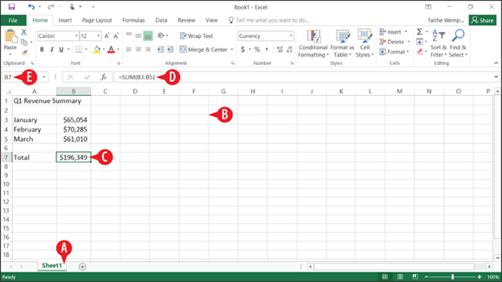
Figure 7-1: Cells are at the intersections of rows and columns.

Excel is very much like Word in many ways. Here are some parts that might seem familiar from previous chapters:

The Ribbon is a multi-tabbed toolbar of commands to issue. Click a tab to switch to it.

The Zoom slider controls the magnification of the work area. Drag the slider left or right to zoom out or in.

Clicking File opens Backstage view, where you can save, open, and print files.

Scroll bars enable you to move around in the worksheet.

The Quick Access toolbar provides shortcuts to a few commonly used commands.

Type in the Tell Me What You Want to Do box to ask a question if you don’t know how to do something.

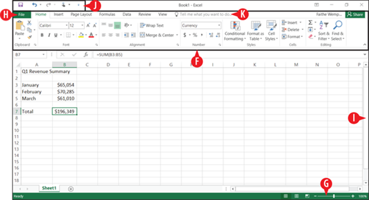
Figure 7-2: Excel has a similar interface to that of other Office applications.

Now that you know what you’re looking at, check out the next several sections, which tell you what you can do with it.

Move between cells

To type in a cell, you must first make that cell active by moving the cell cursor there. As shown earlier in Figure 7-1, the cell cursor is a thick green outline. You can move the cell cursor by pressing the arrow keys on the keyboard, by clicking the desired cell, or by using one of the Excel keyboard shortcuts. Table 7-1 provides some of the most common keyboard shortcuts for moving the cell cursor.

Scrolling with the scroll bar does not change which cell is active; it only changes which cells are visible, but it does not move the cell cursor. One common beginner mistake is to scroll to place the desired cell in view and then start typing without first clicking it to make it active.

Table 7-1 Cell Cursor Movement Shortcuts

* This works only when the Scroll Lock key has been pressed on your keyboard to turn on the Scroll Lock function.

Select cells and ranges

You might sometimes want to select a multi-cell range before you issue a command. For example, if you want to format all the text in a range a certain way, select that range and then issue the formatting command. Technically, a range can consist of a single cell; however, a range most commonly consists of multiple cells. Here are some things to note about cells and ranges:

In Figure 7-3, the range A1:F3 is selected. Range names are written with the upper-left cell address, a colon, and the lower-right cell address.

The active cell is A1. The active cell’s address appears in the Name box.

The active cell within the range appears white, while all the other cells in the selected range are gray.

This points out the difference between the active cell and a multi-cell range. The active cell is significant when doing data entry; when you type text, it goes into the active cell only. The selected range is significant when you are issuing a command, such as applying formatting.

To select a row, click its column letter. Drag across multiple column letters to select multiple columns.

To select a column, click its row number. Drag across multiple row numbers to select multiple rows.

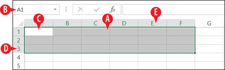
Figure 7-3: The range A1:F3 is selected.

A range is usually contiguous, or all the cells are in a single rectangular block, but they don’t have to be. You can also select noncontiguous cells in a range by holding down the Ctrl key while you select additional cells.

When a range contains noncontiguous cells, the pieces are separated by commas, like this: A1:C3,E3:E5. This range name tells Excel to select the range from A1 through C3, plus the range from E3 through E5. Figure 7-4 shows that range.

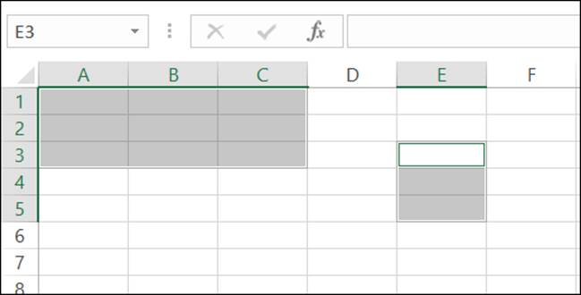
Figure 7-4: A noncontiguous range.

Enter and edit text in cells

Here are some tips for entering and editing text:

To type in a cell, simply select the cell and begin typing. If you make a mistake when editing, you can press the Esc key to cancel the edit before you leave the cell.

Notice that if you type an entry that is wider than the cell, it hangs off into the next column. The solution to that is to widen the column, as you will learn to do in Chapter 8.

When you finish typing, you can leave the cell in any of these ways:

· Press Enter: Moves you to the next cell down.

· Press Tab: Moves you to the next cell to the right.

· Press Shift+Tab: Moves you to the next cell to the left.

· Press an arrow key: Moves you in the direction of the arrow.

· Click in another cell: Moves you to that cell.

If you need to edit the content in a cell, you can click the cell to select it, and then click the cell again to move the insertion point into it. Edit just as you would in any text program. Alternatively, you can click the cell to select it and then type a new entry to replace the old one.

If you need to undo an edit immediately after you leave the cell, click the Undo button on the Quick Access toolbar, or press Ctrl+Z.

To clear a cell, select the cell; then choose Home ⇒ Clear ⇒ Clear Contents.

To clear a cell you can also select it and then either press the Delete key or right-click it and choose Clear Contents.

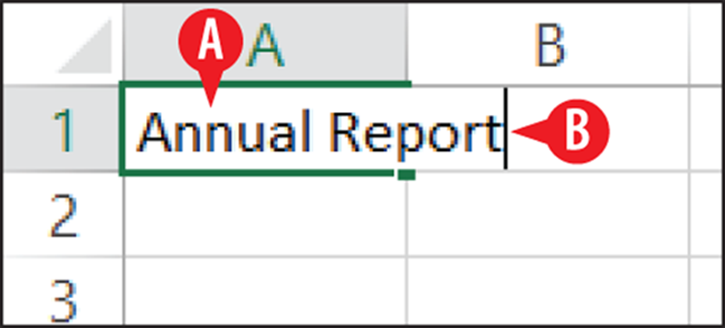
Figure 7-5: Type directly into a cell.

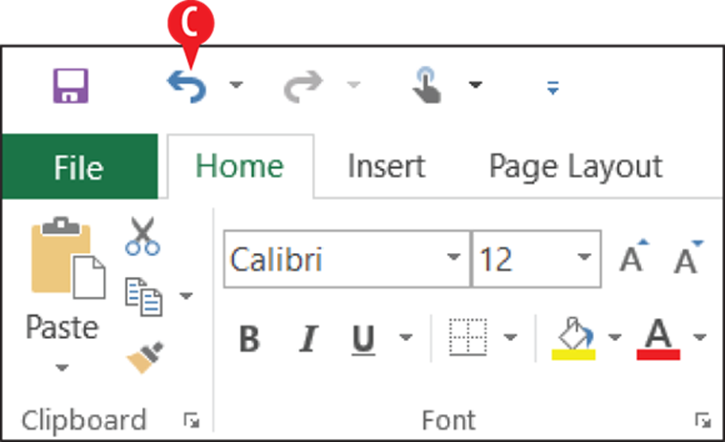
Figure 7-6: Undo an edit

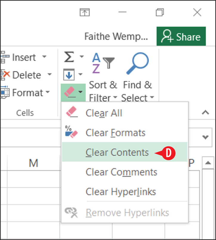
Figure 7-7: Clear a cell’s content.

Don’t confuse the Delete key on the keyboard (which issues the Clear command) with the Delete command on the Ribbon. The Delete command on the Ribbon doesn’t clear the cell content; instead, it removes the entire cell. You find out more about deleting cells in the upcoming section, “Insert and delete rows, columns, and cells.”

And while I’m on the subject, don’t confuse Clear with Cut, either. The Cut command works in conjunction with the Clipboard. Cut moves the content to the Clipboard, and you can then paste it somewhere else. Excel, however, differs from other applications in the way this command works: Using Cut doesn’t immediately remove the content. Instead, Excel puts a flashing dotted box around the content and waits for you to reposition the cell cursor and issue the Paste command. If you do something else in the interim, the cut-and-paste operation is canceled, and the content that you cut remains in its original location. You learn more about cutting and pasting in the section “Copy and move data between cells” later in this lesson.

Use AutoFill to fill cell content

When you have a lot of data to enter and that data consists of some type of repeatable pattern or sequence, you can save time by using AutoFill.

To use AutoFill:

Select the cell or cells that already contain an example of what you want to fill.

Drag the fill handle to extend the selection to the range of cells you want to fill:

The fill handle is the little black square in the lower right corner of the selected cell or range.

As you drag, a ScreenTip appears showing what the value will be in the final cell of the range.

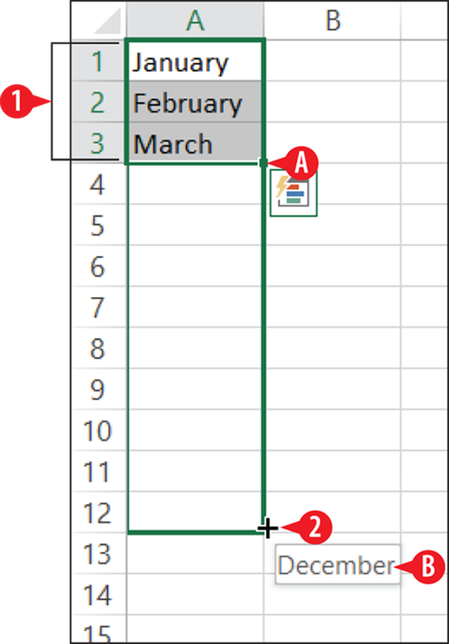
Figure 7-8: Fill a range of cells by dragging the fill handle.

Depending on how you use it, AutoFill can either fill the same value into every cell in the target area, or it can fill in a sequence (such as days of the month, days of the week, or a numeric sequence such as 2, 4, 6, 8). Here are the general rules for how it works:

When AutoFill recognizes the selected text as a member of one of its preset lists, such as days of the week or months of the year, it automatically increments those. For example, if the selected cell contains Monday, AutoFill places Tuesday in the next adjacent cell.

When AutoFill doesn’t recognize the selected text, it fills the chosen cell with a duplicate of the selected text.

When AutoFill is used on a single cell containing a number, it fills with a duplicate of the number.

You can click the AutoFill Options button to open a menu of other choices.

When Auto Fill is used on a range of two or more cells containing numbers, AutoFill attempts to determine the interval between them and continues filling using that same pattern. For example, if the two selected cells contain 2 and 4, the next adjacent cell would be filled with 6.

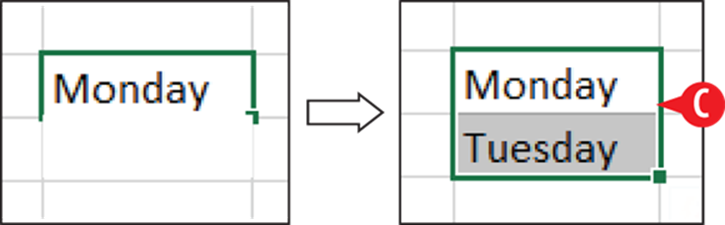
Figure 7-9: AutoFill works on commonly occurring series.

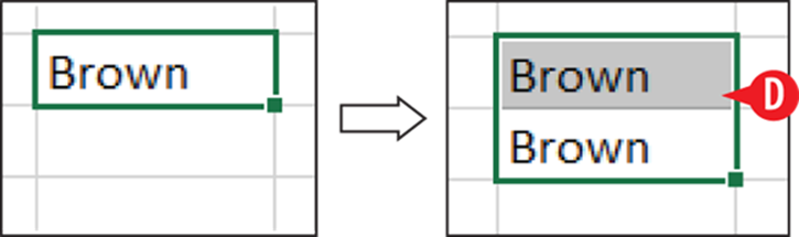
Figure 7-10: AutoFill duplicates the selected text if it’s not a recognized series.

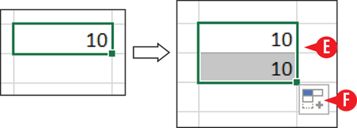
Figure 7-11: AutoFill duplicates a single number.

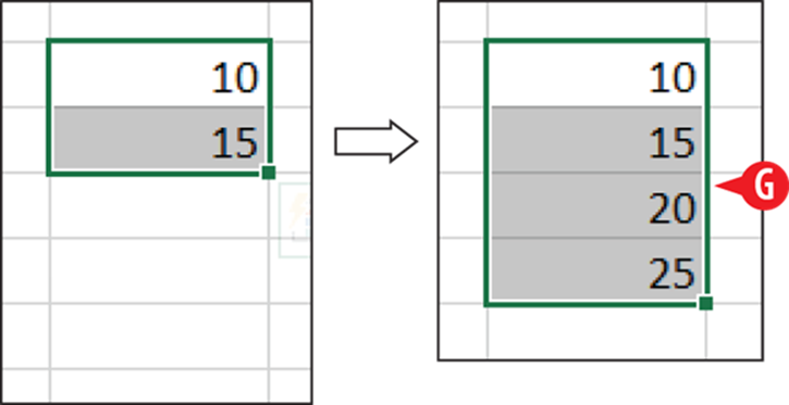
Figure 7-12: AutoFill determines the interval between multiple selected numbers and repeats that pattern.

When you copy formulas or functions (using any method), Excel automatically adjusts the cell references in the copies to the relative positioning of the new locations. For example:

If you have =A1+A2 in cell A3 …

… and you copy A3’s formula into B3 …

… the resulting formula in B3 will be =B1+B2.

This is called relative referencing, and it’s covered in more detail in Chapter 8.

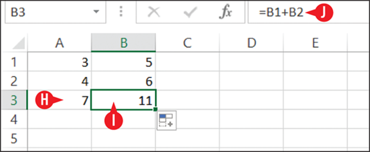
Figure 7-13: AutoFill works when copying formulas and functions.

Copy and move data between cells

When you’re creating a spreadsheet, it’s common not to get everything in the right cells on your first try. Fortunately, moving content between cells is easy.

Here are the two methods you can use to move content: drag it with the mouse or cut/copy and paste using the Clipboard.

Copy and move using the mouse

Moving or copying with the mouse works well when you can see both the source and the destination locations at once. For example, if you want to move a range of cells a few rows up or down, or a few columns to the left or right, this is the method for you. It’s not a good method when moving or copying between different worksheets or workbooks.

To move or copy the contents of a range of cells using the mouse, follow these steps:

Select the range of cells to be moved or copied.

Position the mouse pointer at the dark outline around the selected range. The mouse pointer changes to a four-headed arrow with a white arrow pointer on top of it.

3. (Optional) If you want to copy (not move), hold down the Ctrl key and keep it down until you are finished with step 4. If you do this, the mouse pointer changes to a white arrow pointer with a small plus sign on it.

Drag the selection outline to the new location.

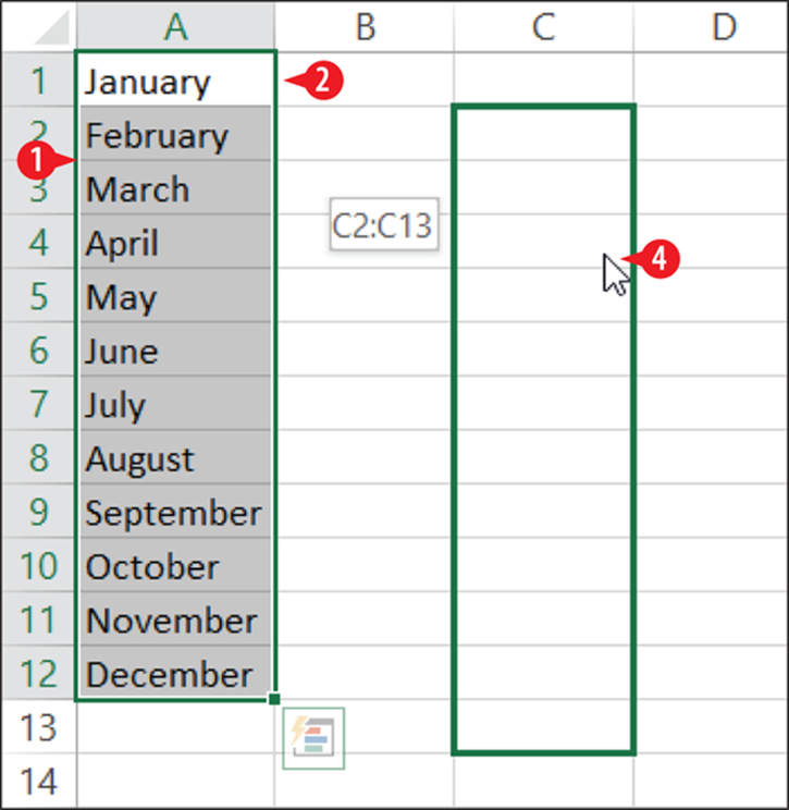
Figure 7-14: Drag a selected range to a new location using the mouse.

Copy and move using the Clipboard

The Clipboard is a temporary holding area in Windows, designed for moving and copying content from one location to another. That statement is intentionally very broad because the Clipboard works with just about any type of content. You can use it to move files from one folder to another, or to move a selection of data in an application (like Excel) from one spot to another in the same data file or a different one.

You can think of the Clipboard like a real-life clipboard. You place something on it for temporary holding, and then when you get to the desired location, you retrieve the item.

The Clipboard works via a combination of the following commands:

· Cut: Removes the item from its original location and places it on the Clipboard.

· Copy: Places a copy of the item on the Clipboard, leaving the original in place.

· Paste: Places a copy of whatever is on the Clipboard in the active location.

To copy, you use a combination of Copy and Paste; to Move, use Cut and Paste:

Select the range of cells to copy or move.

On the Home tab, click Copy (to copy) or Cut (to move). The border around the selection becomes dashed temporarily.

3. Click in the cell that is in the upper-left corner of the area into which you want to paste.

If you’re moving or copying a multi-cell range with the Clipboard, you can either select the same size and shape of range for the destination in step 3 or you can select a single cell, in which case the paste occurs with the selected cell in the upper-left corner.

On the Home tab, click Paste.

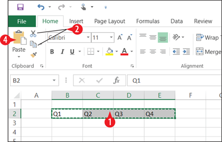
Figure 7-15: Cut or copy, and then paste.

Because the Clipboard is such a popular tool, there are many ways to use it. Table 7-2 summarizes the different ways to issue each of the three basic Clipboard commands.

Table 7-2 Methods of Cutting, Copying, and Pasting with the Clipboard

Insert and delete rows, columns, and cells

Even if you’re a careful planner, you’ll likely decide that you want to change your worksheet’s structure. Maybe you want data in a different column, or certain rows turn out to be unnecessary. Excel makes it easy to insert and delete rows and columns to deal with these kinds of changes.

Insert rows or columns

When you insert a new row or column, the existing ones move to make room for it.

Select one or more existing rows or columns adjacent to where you want the inserted ones. For example, if you want two new columns, select two adjacent existing columns. See “Select cells and ranges” earlier in this chapter for help if needed.

There is no limit on the number of rows or columns you can insert at once.

On the Home tab, click Insert.

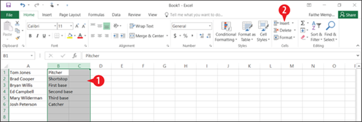
Figure 7-16: Insert rows or columns with the Insert command.

Delete rows or columns

When you delete rows or columns, whatever they contained is lost, so be careful with this command. Delete is not the same as Cut. Cut moves the content to the Clipboard, but Delete just destroys it.

If you accidentally delete something you meant to keep, use Undo (Ctrl+Z) to undo commands until you get it back. This works only if you haven’t closed the application or the data file since you made the deletion.

3. Select one or more existing rows or columns to delete. See “Select cells and ranges” earlier in this chapter for help if needed.

There is no limit on the number of rows or columns you can delete at once.

On the Home tab, click Delete.

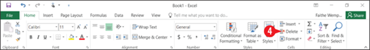
Figure 7-17: Delete rows or columns with the Delete command.

Insert or delete cells and ranges

You can also insert and delete individual cells or even ranges that don’t neatly correspond to entire rows or columns. When you do so, the surrounding cells shift. In the case of an insertion, cells move down or to the right of the area where the new cells are being inserted. In the case of a deletion, cells move up or to the left to fill in the voided space.

Deleting a cell is different from clearing a cell’s content, and this becomes apparent when you start working with individual cells and ranges. When you clear the content, the cell itself remains. When you delete the cell itself, the adjacent cells shift.

When shifting cells, Excel is smart enough that it tries to guess which direction you want existing content to move when you insert or delete cells. If you have content immediately to the right of a deleted cell, for example, Excel shifts it left. If you have content immediately below the deleted cell, Excel shifts it up. You can still override that, though, as needed.

To insert cells:

Select a range the size and shape of the range of cells you want to insert, adjacent to where you want to insert them. To insert a single cell, select a single cell.

On the Home tab, click the arrow on the Insert button to open its menu.

Click Insert Cells.

In the Insert dialog box, specify how you want the adjacent cells to move.

Click OK.

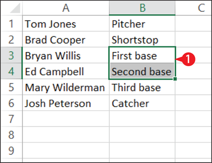
Figure 7-18: Select a range where you want to insert cells.

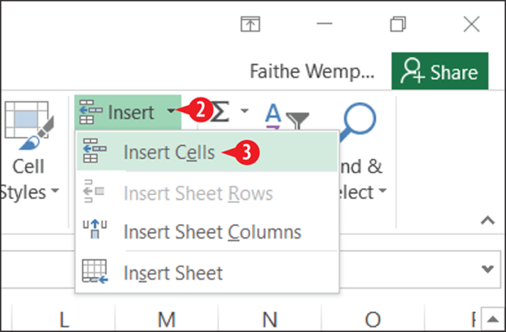
Figure 7-19: Choose Insert Cells from the Insert button’s menu.

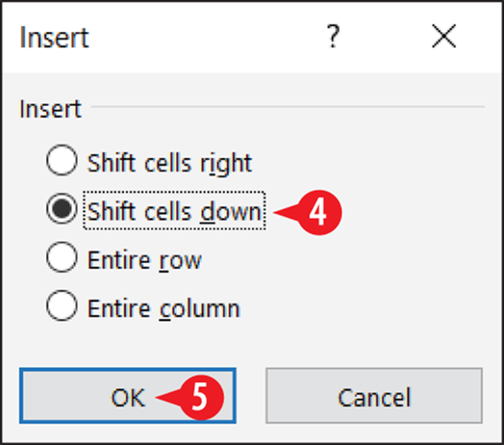
Figure 7-20: Choose where existing content will move to make room for the new cells.

To delete a range of cells or an individual cell:

1. Select the cell(s) to delete.

On the Home tab, click the arrow on the Delete button to open its menu.

Click Delete Cells.

In the Insert dialog box, specify how you want the adjacent cells to move.

Click OK.

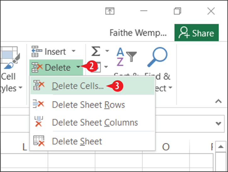
Figure 7-21: Choose Delete Cells from the Delete button’s menu.

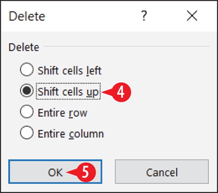
Figure 7-22: Choose where existing content will move when the deleted cells are removed.

Use Flash Fill to extract content

The Flash Fill feature enables you to extract data from adjacent columns intelligently by analyzing the patterns in that data. For example, suppose you have a list of email addresses in one column, and you would like the usernames (that is, the text before the @ sign) from each email address to appear in an adjacent column. You would extract the first few yourself by manually typing the entries into the adjacent column, and then you would use Flash Fill to follow your example to extract the others. You could also use Flash Fill to separate first and last names that are entered in the same column.

To use Flash Fill, follow these steps:

1. Make sure there are enough blank columns to the right of the original data to hold the extracted data. See “Insert and delete rows, columns, and cells” earlier in this chapter if you need help.

In the first row of the data, create an example of the separation you want by typing in the empty column(s).

In the second row of the data, click in the cell in the column you want to populate.

On the Home tab, click the Fill button to open a menu.

Click Flash Fill.

The data in the column you selected in step 3 is filled in. (See in Figure 7-24.)

6. Repeat steps 3-5 as needed to populate additional columns.

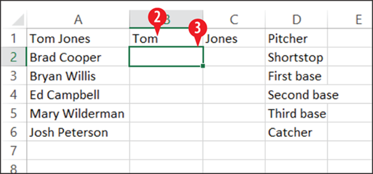
Figure 7-23: Create an example of the separation you want in blank column(s) to the right of the original data.

Step 6 is necessary because you can only Flash Fill one column at a time. If you want to split out data from multiple columns at once, use the Data ⇒ Text to Columns command. Use the Help system in Excel to find out how to use that command.

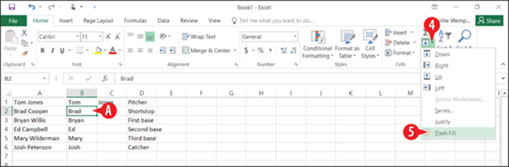
Figure 7-24: The Flash Fill command populates the columns with data using your example.

Create and manage multiple worksheets

Each new workbook starts with one sheet — Sheet1. (Not the most interesting name, but you can change it.) Each worksheet is represented by a tab at the bottom of the Excel window; you can click a tab to switch to that sheet.

You can add or delete worksheets, rearrange the worksheet tabs, and apply different colors to the tabs to help differentiate them from one another, or to create logical groups of tabs.

Add a worksheet

Adding a worksheet gives you an additional page on which to enter your data without having to start a new data file. To add a worksheet:

Click the tab that the new worksheet’s tab should appear to the right of. If your current workbook has only one sheet in it, this is a non-issue.

It’s kind of a non-issue anyway, because you can easily reorder the tabs later. See “Reorder worksheet tabs” later in this chapter.

Click the New Sheet button (+) to the right of the existing sheet tabs at the bottom of the Excel window.

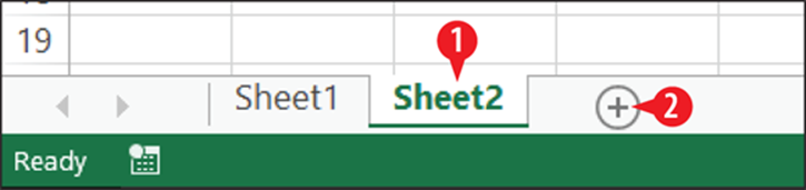
Figure 7-25: Add a worksheet.

Remove a worksheet

Be careful when removing worksheets; whatever was on that sheet is lost when you do so, and you can’t use Undo to get it back. If you are deleting a blank sheet, Excel offers no warning, but if the sheet contains anything, you must confirm the deletion.

To delete a worksheet:

Right-click the worksheet’s tab at the bottom of the screen.

Click Delete.

If a deletion confirmation dialog box appears, click Delete.

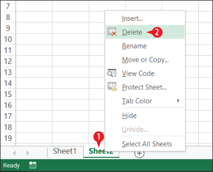
Figure 7-26: Delete a worksheet.

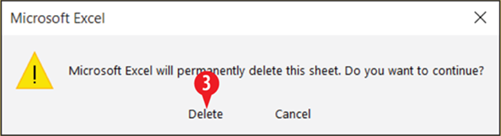
Figure 7-27: Confirm the deletion if the sheet you are deleting is not empty.

Rename a worksheet

As I mentioned earlier, the default sheet names are not terribly useful (Sheet1, Sheet2). You will probably want to rename each sheet’s tab to help you remember what is stored on that sheet.

1. Double-click the worksheet tab to place the name in editing mode. Alternatively, you can right-click the tab and choose Rename.

Edit the name or type a new name.

3. Click away from the tab to accept the new name.

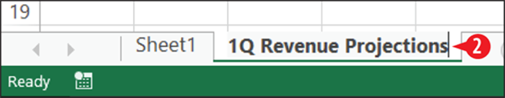
Figure 7-28: Edit the tab’s name.

Reorder worksheet tabs

The tab for a new worksheet is always placed to the right of whichever worksheet is active when you create it. You can easily reorder the worksheet tabs, though.

Drag a tab to the right or left to move it.

A small black triangle shows where the worksheet tab will be dropped when you release the mouse button.

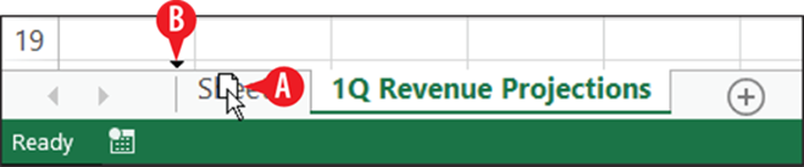
Figure 7-29: Drag a tab to the right or left.

Change the worksheet tab color

If you have a lot of worksheets in a workbook, it can get confusing when you are trying to find the one you want. You can make it easier by color-coding your tabs: gold for management, blue for medical, red for security, and so on. (Yes, those are the Star Trek colors. Use your own scheme.)

To change a tab’s color:

Right-click the tab.

Point to Tab Color.

Click the desired color.

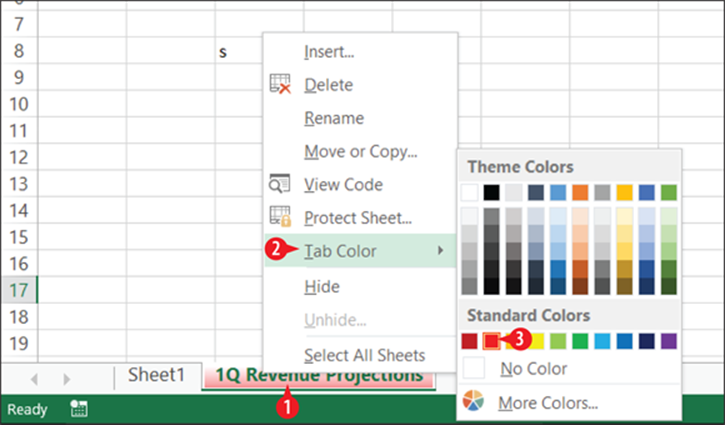
Figure 7-30: Assign a color to a tab to categorize it.